Physical Layer Security for Two-Way Untrusted Relaying with Friendly Jammers

Abstract

In this paper, we consider a two-way relay network where two sources can communicate only through an untrusted intermediate relay, and investigate the physical layer security issue of this two-way relay scenario. Specifically, we treat the intermediate relay as an eavesdropper from which the information transmitted by the sources needs to be kept secret, despite the fact that its cooperation in relaying this information is essential. We indicate that a non-zero secrecy rate is indeed achievable in this two-way relay network even without external friendly jammers. As for the system with friendly jammers, after further analysis, we can obtain that the secrecy rate of the sources can be effectively improved by utilizing proper jamming power from the friendly jammers. Then, we formulate a Stackelberg game model between the sources and the friendly jammers as a power control scheme to achieve the optimized secrecy rate of the sources, in which the sources are treated as the sole buyer and the friendly jammers are the sellers. In addition, the optimal solutions of the jamming power and the asking prices are given and a distributed updating algorithm to obtain the Stakelberg equilibrium is provided for the proposed game. Finally, the simulations results verify the properties and the efficiency of the proposed Stackelberg game based scheme.

I Introduction

Traditionally security in wireless networks has been mainly considered at higher layers using cryptographic methods. However, recent advances in wireless decentralized and ad-hoc networking have led to an increasing attention on studying physical layer based security. The basic idea of physical layer security is to exploit the physical characteristics of the wireless channel to provide secure communication. The security is quantified by the secrecy capacity, which is defined as the maximum rate of reliable information sent from the source to the intended destination in the presence of eavesdroppers. This line of work was pioneered by Aaron Wyner, who introduced the wiretap channel and established fundamental results of creating perfectly secure communications without relying on private keys [1]. Wyner showed that when the eavesdropper channel is a degraded version of the main channel, the source and the destination can exchange perfectly secure messages at a non-zero rate. In follow-up work [2], the secrecy capacity of Gaussian wiretap channel was studied, and in [3] Wyner’s approach was extended to the transmission of confidential messages over broadcast channels. Recently, researches on physical layer security have generalized these studies to wireless fading channels [4, 5, 6, 7], MIMO channels [8, 9, 10, 11, 12], and various multiple access scenarios [13, 14, 15, 16, 17, 18].

Motivated the fact that if the source-wiretapper channel is less noisy than the source-destination channel, the perfect secrecy capacity will be zero [3], some recent work has been proposed to overcome this limitation using relay cooperation, which mainly consists of cooperative relaying [19, 20], and cooperative jamming [21, 22]. For instance, in [19] and [20], the authors proposed effective decode-and-forward (DF) and amplify-and-forward (AF) based cooperative relaying protocols for physical layer security, respectively. Cooperative jamming is another approach to improve the secrecy capacity by distracting the eavesdropper with codewords independent of the source messages. In [21] and [22], several cooperative jamming schemes were investigated for different scenarios, where classical relay strategies fail to offer positive performance gains. Relay channel with confidential messages was studied in [23] and [24], where the relay node acts both as an eavesdropper and a helper. In [25], it was established that cooperation even with an untrusted relay node could be beneficial in relay channels with orthogonal components. Then in [26], the authors considered a two-hop communication system using an untrusted relay and showed that a cooperative jammer enables a positive secrecy capacity which would be otherwise impossible.

Two-way communication is a common scenario where two terminals transmit information to each other simultaneously. Recently, the two-way relay channel [27, 28, 29, 30, 31] has attracted lots of interest from both academic and industrial communities due to its advantage in saving bandwidth efficiently. In [27] and [28], both AF and DF protocols for one-way relay channels were extended to general full-duplex discrete two-way relay channel and half-duplex Gaussian two-way relay channel, respectively. In [29], different relay strategies consisting of AF, DF, and EF (estimate-and-forword) for uncoded two-way relay channels were investigated. In [30], analogue network coding based two-way relay channel with linear processing was analyzed and an optimal relay beamforming structure was presented. In [31], a joint network-channel coding was proposed for the two-way relay channel, where channel codes are used at both the sources and a network code is used at the intermediate relay. Although two-way relay networks have received so much attention so far, the security issue about the relay, especially from the physical layer security point of view, has not been well investigated.

To improve the security in two-way relay channel, distributed protocols are desired. Game theory [32] offers a formal analytical framework with a set of mathematical tools to study the complex interactions among interdependent rational players. Recently, there has been significant growth in research activities that use game theory for analyzing communication networks, mainly due to the need for developing autonomous, distributed, and flexible mobile networks where the network devices can make independent and rational strategic decisions, as well as the need for low complexity distributed algorithms for competitive or collaborative scenarios [33]. In [34] and [35], the authors introduced some recent studies on signal processing and communication networks using game theory. In [36] and [37], the authors employed game theory to physical layer security to study the interaction between the source and the jammers who assist the source by distracting the eavesdropper, and got some distributed game solutions. For two-way relay networks, it is desirable to study the physical layer security problems with the aid of game theory similar to those for one-way relay cases.

In this paper, we investigate physical layer security issues in a two-way relay network with friendly jammers. The two sources can exchange information only through an untrusted relay, as there is no direct communication link between them. The untrusted AF relay acts as both an essential relay and a malicious eavesdropper that has the incentive to eavesdrop on the information transmission. For convenience and ease of comparison, we first study the system without friendly jammers as a special case. We find that a non-zero secrecy rate here is indeed available even without the help of friendly jammers. We also derive an optimal power vector of the relay and the sources by maximizing the secrecy rate. We further investigate the two-way relay secure communication with friendly jammers, and find that a positive gain can be obtained in the secrecy rate by utilizing proper jamming power from the friendly jammers. Then the problem comes to how to effectively utilize the jamming power from different friendly jammers to maximize the secrecy rate. Thus, we propose a Stackelberg game model between the sources and the friendly jammers as a power control scheme. In the defined game, the sources pay the friendly jammers for interfering the untrusted relay in order to increase the secrecy rate, while the friendly jammers charge the sources with a certain price for their service of jamming. In addition, the optimal solutions of the jamming power and the asking prices are given and a distributed updating algorithm to obtain the Stakelberg equilibrium is provided for the proposed game. Furthermore, a centralized scheme is also proposed for comparison with the distributed Stackelberg game based scheme. Finally, the proposed approaches and solutions are verified by simulations.

The rest of this paper is organized as follows. In Section II, the system model of two-way relay communication with friendly jammers is described and the corresponding secrecy rate is formulated. In Section III, a two-way relay system without jammers as a special case is investigated. In Section IV, we define a Stackelberg type of buyer/seller game to investigate the interaction between the sources and the friendly jammers, and analyze the optimization problem of physical layer security in the presence of friendly jammers. Simulation results are provided in Section V, and the conclusions are drawn in Section VI.

II System Model

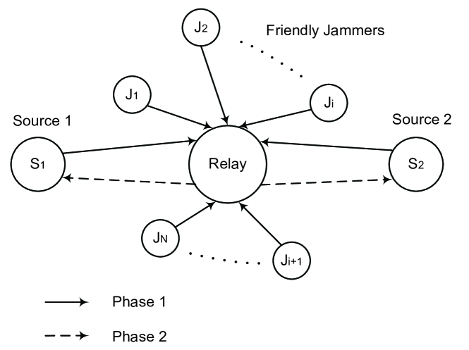
Figure 1: System model for two-way relay communications with friendly jammers

As shown in Fig. 1, we consider a basic two-way relay network consisting of two source nodes, one untrusted relay node, and $N$ friendly jammer nodes, which are denoted by $S_{k}$, $k=1,2$, $R$, and $J_{i}$, $i=1,2,\ldots,N$, respectively. We denote by $\mathcal{N}$ the set of indices $\{1,2,\ldots,N\}$. All the nodes here are equipped with only a single omni-directional antenna and operate in a half-duplex way, i.e., each node cannot receive and transmit simultaneously. Then the complete transmission can be divided into two phases. During the first phase, shown with solid lines, both source nodes transmit their information to the relay node. Simultaneously, the friendly jammers also transmit the jamming signals in order to distract the malicious relay. In the second phase, shown with dashed lines, the relay node broadcasts a combined version of the received signals to both source nodes. Note that in the system we investigate there is only one intermediate relay and we assume that no direct link exists between the two sources. Thus, the sole untrusted relay is necessary for the two-way relaying data transmission. A key assumption we make here is that the sources have perfect knowledge of the jamming signals transmitted by the friendly jammers, for they have paid for the service.

Let $s_{1}$, $s_{2}$, and $s_{i}^{J}$, $i\in\mathcal{N}$, denote the signal to be transmitted by the source $S_{1},S_{2}$, and the jammers $J_{i}$, $i\in\mathcal{N}$, respectively. Suppose source nodes $S_{1}$ and $S_{2}$ transmit with power $p_{1}$ and $p_{2}$, and the channel gains from the source nodes to the relay node are denoted by $h_{S_{k},R}$, $k=1,2$. Each friendly jammer node $i$ transmits with power $p_{i}^{J}$, and the channel gain from it to the relay node is denoted by $h_{J_{i},R}$, $i\in\mathcal{N}$. The channel gain contains the path loss and the Rayleigh fading coefficient with zero mean and unit variance. For simplicity, we assume that the fading coefficients are constant over one frame, and vary independently from one frame to another.

In phase $1$, the received signal at the malicious relay can be expressed as

$${y_{r}}=n_{r}+\sqrt{p_{1}}s_{1}h_{S_{1},R}+\sqrt{p_{2}}s_{2}h_{S_{2},R}+\sum_{i}\sqrt{p_{i}^{J}}s_{i}^{J}h_{J_{i},R},$$ (1)

where $n_{r}$ denotes the thermal noise at the relay node $R$, which is a zero mean Gaussian random variable with two sided power spectral density of $\sigma^{2}$, i.e., $\mathcal{C}\mathcal{N}(0,\sigma^{2})$. Furthermore, we assume that the noises at $S_{1}$, $S_{2}$, and $R$ are independent and identically distributed (i.i.d.).

In phase $2$, the malicious relay, which works in AF mode, amplifies the received signal $y_{r}$ by a factor $\beta$ and then broadcasts the signal to both $S_{1}$ and $S_{2}$ with power $p_{r}$. The power normalization factor $\beta$ at the relay node can be written as

$${\beta}=\left(p_{1}\left|h_{S_{1},R}\right|{}^{2}+p_{2}\left|h_{S_{2},R}\right|{}^{2}+\sum_{i}p_{i}^{J}\left|h_{J_{i},R}\right|{}^{2}+\sigma^{2}\right)^{-1/2}.$$ (2)

Then the corresponding signal received by the source $S_{1}$ , denoted by $y_{1}$, can be written as

$${y_{1}} =\beta\sqrt{p_{r}}h_{S_{1},R}y_{r}+n_{1}=\xi_{1}s_{1}+\upsilon_{1}s_{2}+\sum_{i}\mu_{1,i}s_{i}^{J}+\omega_{1},$$ (3)

where ${\xi_{1}}\triangleq\beta\sqrt{{p_{r}}{p_{1}}}h_{{S_{1}},R}^{2}$, ${\upsilon_{1}}\triangleq\beta\sqrt{{p_{r}}{p_{2}}}{h_{{S_{1}},R}}{h_{{S_{2}},R}}$, ${\mu_{1,i}}\triangleq\beta\sqrt{{p_{r}}p_{i}^{J}}{h_{{J_{i}},R}}{h_{{S_{1}},R}}$, and ${\omega_{1}}\triangleq\beta\sqrt{{p_{r}}}{h_{{S_{1}},R}}{n_{r}}+{n_{1}}$. Similarly, the signal received by the source $S_{2}$, denoted by $y_{2}$, can be written as

$${y_{2}} =\beta\sqrt{{p_{r}}}{h_{{S_{2}},R}}{y_{r}}+{n_{2}}={\xi_{2}}{s_{1}}+{\upsilon_{2}}{s_{2}}+\sum\limits_{i}{{\mu_{2,i}}s_{i}^{J}}+{\omega_{2}},$$ (4)

where ${\xi_{2}}\triangleq\beta\sqrt{{p_{r}}{p_{1}}}{h_{{S_{1}},R}}{h_{{S_{2}},R}}$, ${\upsilon_{2}}\triangleq\beta\sqrt{{p_{r}}{p_{2}}}h_{{S_{2}},R}^{2}$, ${\mu_{2,i}}\triangleq\beta\sqrt{{p_{r}}p_{i}^{J}}{h_{{J_{i}},R}}{h_{{S_{2}},R}}$, and ${\omega_{2}}\triangleq\beta\sqrt{{p_{r}}}{h_{{S_{2}},R}}{n_{r}}+{n_{2}}$.

Assuming that both the source nodes and the jammer nodes are independent, from (1), in phase $1$, using the matched filter (MF) , the untrusted relay node has the capacity with respect to $S_{1}$ and $S_{2}$ as

$${C_{1}^{m}}=\frac{W}{2}\log\left({1+\frac{{{p_{1}}{g_{{S_{1}},R}}}}{{{\sigma^{2}}+{p_{2}}{g_{{S_{2}},R}}+\sum\limits_{i}{p_{i}^{J}{g_{{J_{i}},R}}}}}}\right),$$ (5)

and

$${C_{2}^{m}}=\frac{W}{2}\log\left({1+\frac{{{p_{2}}{g_{{S_{2}},R}}}}{{{\sigma^{2}}+{p_{1}}{g_{{S_{1}},R}}+\sum\limits_{i}{p_{i}^{J}{g_{{J_{i}},R}}}}}}\right),$$ (6)

where $W$ represents the channel bandwidth, ${g_{{S_{1}},R}}\triangleq{\left|{{h_{{S_{1}},R}}}\right|^{2}}$, ${g_{{S_{2}},R}}\triangleq{\left|{{h_{{S_{2}},R}}}\right|^{2}}$, and ${g_{{J_{i}},R}}\triangleq{\left|{{h_{{J_{i}},R}}}\right|^{2}}$, $i\in\mathcal{N}$.

In phase $2$, at $S_{1}$, as $s_{1}$ as well as $s_{i}^{J}$ is known to the source node, and thus we have

$$\tilde{y}_{1}={\upsilon_{1}}{s_{2}}+{\omega_{1}}.$$ (7)

Then, the corresponding SNR for the transmission from $S_{2}$ to $S_{1}$, denoted by $\gamma_{2}$, can be expressed as

$${\gamma_{2}} =\frac{{{{\left|{{\upsilon_{1}}}\right|}^{2}}}}{{Var\left\{{{\omega_{1}}}\right\}}}=\frac{{{p_{2}}{g_{{S_{2}},R}}}}{{{\sigma^{2}}+{K_{2}}+\sum\limits_{i}{\frac{{{\sigma^{2}}{g_{{J_{i}},R}}}}{{{p_{r}}{g_{{S_{1}},R}}}}p_{i}^{J}}}},$$ (8)

where ${K_{2}}=\frac{{{\sigma^{2}}({p_{1}}{g_{{S_{1}},R}}+{p_{2}}{g_{{S_{2}},R}}+{\sigma^{2}})}}{{{p_{r}}{g_{{S_{1}},R}}}}$. Similarly, at $S_{2}$, the received signal with $s_{2}$ and $s_{i}^{J}$ removed can be written as

$$\tilde{y}_{2}={\xi_{2}}{s_{1}}+{\omega_{2}}.$$ (9)

The corresponding SNR for the transmission from $S_{1}$ to $S_{2}$, denoted by $\gamma_{1}$, can be expressed as

$${\gamma_{1}} =\frac{{{{\left|{{\xi_{2}}}\right|}^{2}}}}{{Var\left\{{{\omega_{2}}}\right\}}}=\frac{{{p_{1}}{g_{{S_{1}},R}}}}{{{\sigma^{2}}+{K_{1}}+\sum\limits_{i}{\frac{{{\sigma^{2}}{g_{{J_{i}},R}}}}{{{p_{r}}{g_{{S_{2}},R}}}}p_{i}^{J}}}},$$ (10)

where ${K_{1}}=\frac{{{\sigma^{2}}\left({{p_{1}}{g_{{S_{1}},R}}+{p_{2}}{g_{{S_{2}},R}}+{\sigma^{2}}}\right)}}{{{p_{r}}{g_{{S_{2}},R}}}}$.

Capacities of two-way relay channel between the two sources are denoted by $C_{1}$ and $C_{2}$, and we have

$${C_{1}}=\frac{W}{2}\log\left({1+{\gamma_{1}}}\right),$$ (11)

and

$${C_{2}}=\frac{W}{2}\log\left({1+{\gamma_{2}}}\right).$$ (12)

Then, the secrecy rate for $S_{1}$ and $S_{2}$ [5] can be defined as

$${C_{1}^{s}}={\left({{C_{1}}-C_{1}^{m}}\right)^{+}},$$ (13)

and

$${C_{2}^{s}}={\left({{C_{2}}-C_{2}^{m}}\right)^{+}},$$ (14)

where ${\left(x\right)^{+}}$ represents $\max\left\{{x,0}\right\}$. According to [25] and [26], we have that the defined secrecy rate is achievable in a two-hop secure communication with an untrusted relay.

As a special case, if the jammers are not used, the jammers’ transmit power $p_{i}^{J}$ should be set to zero, $\forall i\in\mathcal{N}$. Then from the derivation above, we can get the corresponding secrecy rate in this case as

$${\tilde{C}_{1}^{s}}=\frac{W}{2}{\left[{\log\left({1+\frac{{{p_{1}}{g_{{S_{1}},R}}}}{{{\sigma^{2}}+{K_{1}}}}}\right)-\log\left({1+\frac{{{p_{1}}{g_{{S_{1}},R}}}}{{{\sigma^{2}}+{p_{2}}{g_{{S_{2}},R}}}}}\right)}\right]^{+}},$$ (15)

and

$${\tilde{C}_{2}^{s}}=\frac{W}{2}{\left[{\log\left({1+\frac{{{p_{2}}{g_{{S_{2}},R}}}}{{{\sigma^{2}}+{K_{2}}}}}\right)-\log\left({1+\frac{{{p_{2}}{g_{{S_{2}},R}}}}{{{\sigma^{2}}+{p_{1}}{g_{{S_{1}},R}}}}}\right)}\right]^{+}}.$$ (16)

In the system we investigate, there is only one intermediate relay, thus this sole relay is necessary in our assumption for two-way relaying data transmission. Actually, the untrusted relay has the incentive to forward the signals from both the sources since it can eavesdrop on the information transmission through this kind of cooperation. If the relay is non-cooperative that it only receives but not relays the information, then the problem comes to deny-of-service attack. However, this can be easily detected by the sources, then the non-cooperative relay will be treated as a thorough eavesdropper and lose the good opportunity to eavesdrop on the information transmission. The sources will then turn to another intermediate relay for help to relay their information in a practical scenario where there exist multiple intermediate relays. In this paper, we focus on the studies how to prevent the untrusted but necessary intermediate relay from eavesdropping the information, and thus, for simplicity and without loss of generality, we assume that there is only one necessary intermediate relay in the system and the relay is cooperative.

III Secrecy Rate of Two-Way Relay Channel Without Jammers

For comparison and consistence, we first investigate the special case without the presence of jammers in this section. We prove that there indeed exists a positive secrecy rate for the two-way relay channel even without the help of friendly jammers distracting the malicious relay. Furthermore, we also obtain an optimal power allocation of the sources and the relay to maximize the secrecy rate. In the next section, we will compare the case with friendly jammers with this case to expect a positive performance gain in the secrecy rate.

III-A Existence of Non-zero Secrecy Rate

When the eavesdropper channels from the two sources to the malicious relay are degraded versions of the equivalent main two-way relay channel between $S_{1}$ and $S_{2}$, the two sources can exchange perfectly secure messages at a non-zero rate. Firstly, we consider the transmission from $S_{1}$ to $S_{2}$. In phase $1$, the malicious relay receives the signal $s_{1}$ from $S_{1}$, which consists of the information for $S_{2}$. Meanwhile, $S_{2}$ also transmits the signal $s_{2}$ at the relay, which acts as both the information carrier for $S_{1}$ and a jamming signal that makes the eavesdropper channel from $S_{1}$ to the malicious relay getting worse. In phase $2$, the combined signal consisting of $s_{1}$ and $s_{2}$ arrives at $S_{2}$. As $S_{2}$ has a perfect knowledge of its own signal $s_{2}$, the signal that jammed the malicious relay in phase $1$ has no such an effect on $S_{2}$. Therefore, it makes possible that the eavesdropper channel is worse than the data transmission channel from $S_{1}$ to $S_{2}$, which means that a non-zero rate for secure communication from $S_{1}$ to $S_{2}$ is available. It is the same situation in the transmission from $S_{2}$ to $S_{1}$. From (15), (16) and the expressions of $K_{1}$ in (10) and $K_{2}$ in (8), we can write the probability of the existence of a non-zero secrecy rate as

$${\rm P}\left({\tilde{C}_{1}^{s}>0,\tilde{C}_{2}^{s}>0}\right) ={\rm P}\left({{K_{1}}<{p_{2}}{g_{{S_{2}},R}},{K_{2}}<{p_{1}}{g_{{S_{1}},R}}}\right)$$

$$={\rm P}\left({{p_{r}}>\max\left\{{\frac{T}{{{p_{2}}g_{{S_{2}},R}^{2}}},\frac{T}{{{p_{1}}g_{{S_{1}},R}^{2}}}}\right\}}\right),$$ (17)

where $T=({p_{1}}{g_{{S_{1}},R}}+{p_{2}}{g_{{S_{2}},R}}+{\sigma^{2}}){\sigma^{2}}$.

Considering the power constraints ${p_{1}}\leq{p_{max}}$, ${p_{2}}\leq{p_{max}}$, and ${p_{r}}\leq{p_{max}}$, we can get that there exists at least one pair of $\left({{p_{r}},{p_{1}},{p_{2}}}\right)$ that satisfies ${p_{r}}>\max\left\{{\frac{T}{{{p_{2}}g_{{S_{2}},R}^{2}}},\frac{T}{{{p_{1}}g_{{S_{1}},R}^{2}}}}\right\}$, under the channel condition of $\frac{{{g_{{S_{1}},R}}+{g_{{S_{2}},R}}}}{{{g_{{S_{1}},R}}{g_{{S_{2}},R}}}}<\frac{{{p_{max}}}}{{{\sigma^{2}}}}$. Therefore, we have ${\rm P}\left({\tilde{C}_{1}^{s}>0,\tilde{C}_{2}^{s}>0}\right)>0$ at some power vectors of $\left({{p_{r}},{p_{1}},{p_{2}}}\right)$, which actually indicates that a non-zero secrecy rate in the two-way relay channel is indeed available.

III-B Maximizing the Secrecy Rate

In this subsection, we try to get an optimal power vector of $\left({{p_{r}},{p_{1}},{p_{2}}}\right)$ which maximizes the secrecy rate of the two-way relay channel. We can formulate the problem subject to the individual secrecy rate constraints and power constraints as

$$\max\;{\tilde{C}^{s}}=\max\;\sum\limits_{k=1}^{2}{\tilde{C}_{k}^{s}},$$ (18)

s.t. $$\left\{\begin{array}[]{l}\tilde{C}_{1}^{s}>0,\>\tilde{C}_{2}^{s}>0\\ {p_{1}}\leq{p_{max}},\>{p_{2}}\leq{p_{max}},\>{p_{r}}\leq{p_{max}}\\ \end{array}\right..$$ (21)

From (III-A), we have that

$$\tilde{C}_{1}^{s}>0,\;\tilde{C}_{2}^{s}>0\Leftrightarrow{p_{r}}>\max\left\{{\frac{T}{{{p_{2}}g_{{S_{2}},R}^{2}}},\frac{T}{{{p_{1}}g_{{S_{1}},R}^{2}}}}\right\}.$$ (22)

From (15), (16), and (18), we can get that

$${\tilde{C}^{s}}=\frac{W}{2}{\left({\log\tilde{F}\left({{p_{r}},{p_{1}},{p_{2}}}\right)}\right)^{+}},$$ (23)

where

$$\tilde{F}\left({{p_{r}},{p_{1}},{p_{2}}}\right)\triangleq\frac{{\left({1+\frac{{{p_{1}}{g_{{S_{1}},R}}}}{{{\sigma^{2}}+{K_{1}}}}}\right)\left({1+\frac{{{p_{2}}{g_{{S_{2}},R}}}}{{{\sigma^{2}}+{K_{2}}}}}\right)}}{{\left({1+\frac{{{p_{1}}{g_{{S_{1}},R}}}}{{{\sigma^{2}}+{p_{2}}{g_{{S_{2}},R}}}}}\right)\left({1+\frac{{{p_{2}}{g_{{S_{2}},R}}}}{{{\sigma^{2}}+{p_{1}}{g_{{S_{1}},R}}}}}\right)}}.$$ (24)

As $\tilde{F}({p_{r}},{p_{1}},{p_{2}})$ has the same monotonic property as ${\tilde{C}^{s}}$ under the conditions of (18), we can transform the optimization problem as

$$\max\;\tilde{F}\left({{p_{r}},{p_{1}},{p_{2}}}\right),$$ (25)

s.t. $$\left\{\begin{array}[]{l}{p_{r}}>\max\left\{{\frac{T}{{{p_{2}}g_{{S_{2}},R}^{2}}},\frac{T}{{{p_{1}}g_{{S_{1}},R}^{2}}}}\right\}\\ {p_{1}}\leq{p_{max}},\>{p_{2}}\leq{p_{max}},\>{p_{r}}\leq{p_{max}}\\ \end{array}\right..$$ (28)

It can be calculated that $\frac{{\partial\tilde{F}\left({{p_{r}},{p_{1}},{p_{2}}}\right)}}{{\partial{p_{r}}}}>0$ is always established under the conditions of (25), which implies that $\tilde{F}\left({{p_{r}},{p_{1}},{p_{2}}}\right)$ is a monotonically increasing function of ${p_{r}}$. Therefore, when maximizing the secrecy rate ${\tilde{C}^{s}}$, ${p_{r\_opt}}={p_{max}}$, where ${p_{r\_opt}}$ denotes the optimal relay power . As a result, the problem can be further transformed into $\max\;\tilde{F}\left({{p_{max}},{p_{1}},{p_{2}}}\right)$.

The optimal solutions of $p_{1}$ and $p_{2}$ when maximizing the secrecy rate can be easily obtained under different conditions (i.e., $g_{S_{1},R}>g_{S_{2},R}$, $g_{S_{1},R}<g_{S_{2},R}$, and $g_{S_{1},R}=g_{S_{2},R}$) through the Lagrangian method by solving the Karush-Kuhn-Tucker (KKT) conditions [43]. In this paper, subject to the space limit, we omit the detailed computing process and only give the results of the optimal solutions of $p_{1}$ and $p_{2}$ as:

1. For the case that ${g_{{S_{1}},R}}>{g_{{S_{2}},R}}$, it yields that ${p_{2\_opt}}={p_{max}}$. Meanwhile, if there exists a solution $p_{1}^{*}\in\left({0,{p_{max}}}\right]$ that satisfies the equation $\frac{{\partial\tilde{F}\left({{p_{max}},{p_{1}},{p_{max}}}\right)}}{{\partial{p_{1}}}}=0$, then we have ${p_{1\_opt}}=p_{1}^{*}$. Otherwise, we have ${p_{1\_opt}}={p_{max}}$. Here ${p_{1\_opt}}$ and ${p_{2\_opt}}$ denote the optimal power transmitted by ${S_{1}}$ and ${S_{2}}$, respectively.

2. For the case that ${g_{{S_{1}},R}}<{g_{{S_{2}},R}}$, it yields that ${p_{1\_opt}}={p_{max}}$. Meanwhile, if there exists a solution $p_{2}^{*}\in\left({0,{p_{max}}}\right]$ that satisfies the equation $\frac{{\partial\tilde{F}\left({{p_{max}},{p_{max}},{p_{2}}}\right)}}{{\partial{p_{2}}}}=0$, then we have ${p_{2\_opt}}=p_{2}^{*}$. Otherwise, we have ${p_{2\_opt}}={p_{max}}$.

3. For the case that ${g_{{S_{1}},R}}={g_{{S_{2}},R}}$, we have that ${p_{1\_opt}}={p_{max}}$, and ${p_{2\_opt}}={p_{max}}$.

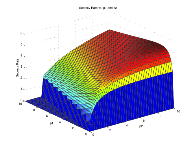
Figure 2: Secrecy rate vs. $p_{1}$ and $p_{2}$ for the case without jammers when ${g_{{S_{1}},R}}>{g_{{S_{2}},R}}$

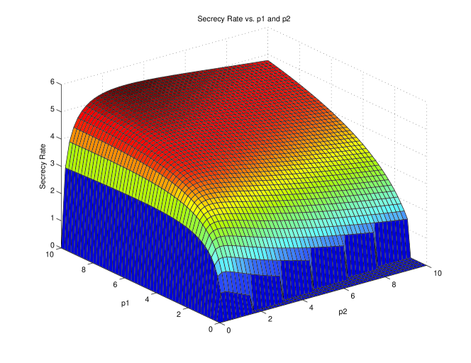
Figure 3: Secrecy rate vs. $p_{1}$ and $p_{2}$ for the case without jammers when ${g_{{S_{1}},R}}<{g_{{S_{2}},R}}$

In addition, we verify these optimal solutions by simulations in different cases which is shown in Fig. 2 and Fig. 3 in Section-V, and after further calculation based on the simulation results, we can get that the results agree with the optimal power solutions well.

IV Physical Layer Security with Friendly Jammers

In this section, through further analysis, we first find that the secrecy rate of the sources can be effectively improved by utilizing proper jamming power from the friendly jammers. Then, the problem comes to how to control the jamming power from different friendly jammers when optimizing the secrecy rate of the sources. In general, in a cooperative wireless network with selfish nodes, nodes may not serve a common goal or belong to a single authority. Thus, a mechanism of reimbursement to the friendly jammers should be employed such that the friendly jammers can earn benefits from spending their own transmitting power in helping the sources for secure data transmission. For the source side, the sources aim to achieve the best performance of secrecy rate with the friendly jammers’ help with the least reimbursements to them. For the friendly jammer side, each friendly jammer aims to earn the payment not only covers its transmitting cost but also gains as many extra profits as possible. Therefore, we employ a Stackelberg game model [32] as a power control scheme jointly considering both the benefits of the sources and the friendly jammers. In the Stackelberg game model we proposed, the two sources as a unity is the sole buyer that starts the process of the proposed Stackelberg game, and the friendly jammers are the sellers, therefore, the sources are treated as leader while the friendly jammers are the followers. Furthermore, the optimal solutions of the jamming power and asking price are investigated and a corresponding distributed updating algorithm is provided. Finally, a centralized scheme is proposed for performance comparison.

IV-A Secrecy Rate Improvement using Friendly Jammers

From (13) and (14), we have

$$C_{1}^{s}=\frac{W}{2}\left[\log\left({1+\frac{{{p_{1}}{g_{{S_{1}},R}}}}{{{\sigma^{2}}+{K_{1}}+\sum\limits_{i}{\frac{{{\sigma^{2}}{g_{{J_{i}},R}}}}{{{p_{r}}{g_{{S_{2}},R}}}}p_{i}^{J}}}}}\right)\right.$$

$$\left.-\log\left({1+\frac{{{p_{1}}{g_{{S_{1}},R}}}}{{{\sigma^{2}}+{p_{2}}{g_{{S_{2}},R}}+\sum\limits_{i}{{g_{{J_{i}},R}}p_{i}^{J}}}}}\right)\right]^{+},$$ (29)

and

$$C_{2}^{s}=\frac{W}{2}\left[\log\left({1+\frac{{{p_{2}}{g_{{S_{2}},R}}}}{{{\sigma^{2}}+{K_{2}}+\sum\limits_{i}{\frac{{{\sigma^{2}}{g_{{J_{i}},R}}}}{{{p_{r}}{g_{{S_{1}},R}}}}p_{i}^{J}}}}}\right)\right.$$

$$\left.-\log\left({1+\frac{{{p_{2}}{g_{{S_{2}},R}}}}{{{\sigma^{2}}+{p_{1}}{g_{{S_{1}},R}}+\sum\limits_{i}{{g_{{J_{i}},R}}p_{i}^{J}}}}}\right)\right]^{+}.$$ (30)

From (IV-A) and (IV-A), we can see that both ${C_{k}}$ and $C_{k}^{m}$, $k=1,2$, are decreasing and convex functions of jamming power $p_{i}^{J}$, $i\in\mathcal{N}$. However, if $C_{k}^{m}$ decreases faster than ${C_{k}}$ as the jamming power $p_{i}^{J}$ increases, $C_{k}^{s}$ might increase in some region of value $p_{i}^{J}$. But when $p_{i}^{J}$ further increases, both ${C_{k}}$ and $C_{k}^{m}$ will approach zero. As a result, $C_{k}^{s}$ approaches zero. Compared to (15) and (16), we can get that if $\frac{{{\sigma^{2}}{g_{{J_{i}},R}}}}{{{p_{r}}{g_{{S_{2}},R}}}}<{g_{{J_{i}},R}}$ and $\frac{{{\sigma^{2}}{g_{{J_{i}},R}}}}{{{p_{r}}{g_{{S_{1}},R}}}}<{g_{{J_{i}},R}}$, $\forall i\in\mathcal{N}$, i.e., $\frac{{{\sigma^{2}}}}{{{p_{r}}}}<\min\left\{{{g_{{S_{1}},R}},{g_{{S_{2}},R}}}\right\}$, the gain of the secrecy rate will be above zero in some region of the jamming power $p_{i}^{J}$. Then the problem comes to how to utilize the jamming power from different friendly jammers effectively to maximize the secrecy rate. Thus, we propose a Stackelberg game model to achieve effective jamming power control in the following subsections.

Note that synchronization among the sources and the friendly jammers is important in the investigated system with friendly jammers. Many works have been devoted to the synchronization issues among distributed nodes in cooperative networks, for example in [44, 45], effective synchronization schemes among distributed sensors and cooperative relays with low complexity and good performance were proposed. Thus, the synchronization issue among the sources and the friendly jammers can be addressed effectively using methods similar to those proposed in [44, 45]. However, this is not the key investigated issue in this paper, therefore, we assume that perfect synchronization among the sources and the friendly jammers is implemented in the system.

IV-B Source Side Game

We consider the two sources as two buyers who want to optimize their secrecy rates, while the cost paid for the “service”, i.e., jamming power $p_{i}^{J}$, $i\in\mathcal{N}$, should also be taken into consideration. For the source side we can define the utility function as

$${U_{s}}=a\left({C_{1}^{s}+C_{2}^{s}}\right)-M,$$ (31)

where $a$ is a positive constant representing the economic gain per unit rate of confidential data transmission between the two sources, and $M$ is the cost to pay for the friendly jammers. Here we have

$$M=\sum\limits_{i\in\mathcal{N}}{{m_{i}}p_{i}^{J}},$$ (32)

where $m_{i}$ is the price per unit power paid for the friendly jammer $i$ by the sources, $i\in\mathcal{N}$.

When considering the optimal transmitting power vector of source $S_{1}$ and $S_{2}$, i.e., $\left({{p_{1}},{p_{2}}}\right)$ to achieve the maximum utility value in (31), we can treat the jamming power $p_{i}^{J}$, $i\in\mathcal{N}$, as constants since all the nodes transmit with independent power. Thus, we can obtain similar results of optimal power solutions as given in Subsection-III-B. But to obtain the optimal solutions of $p_{1}$ and $p_{2}$ is not our main purpose here. In this subsection, we formulate the source side game to study how to effectively utilize the jamming power from different friendly jammers in order to achieve the maximum utility value.

Then the source side game can be expressed as

$$\max\;{U_{s}}=\max\;\left({a\left({C_{1}^{s}+C_{2}^{s}}\right)-M}\right),$$ (33)

s.t. $$\left\{\begin{array}[]{l}C_{1}^{s}\geq 0,C_{2}^{s}\geq 0\\ 0\leq p_{i}^{J}\leq{p_{max}},{p_{r}}={p_{max}},fixed\,{p_{1}},{p_{2}}\\ \end{array}\right..$$ (36)

The goal of the sources as buyers is to buy the optimal amount of power from the friendly jammers in order to maximize the secrecy rate. From (IV-A), (IV-A), and (33), we have

$${U_{s}}= \frac{{aW}}{2}\left({\log\frac{{1+\frac{1}{{{A_{1}}+\sum\limits_{i}{{T_{1,i}}p_{i}^{J}}}}}}{{1+\frac{1}{{{B_{1}}+\sum\limits_{i}{{L_{1,i}}p_{i}^{J}}}}}}+\log\frac{{1+\frac{1}{{{A_{2}}+\sum\limits_{i}{{T_{2,i}}p_{i}^{J}}}}}}{{1+\frac{1}{{{B_{2}}+\sum\limits_{i}{{L_{2,i}}p_{i}^{J}}}}}}}\right)-\sum\limits_{i}{{m_{i}}}p_{i}^{J},$$ (37)

where ${A_{1}}\triangleq\frac{{{\sigma^{2}}+{K_{1}}}}{{{p_{1}}{g_{{S_{1}},R}}}}$, ${A_{2}}\triangleq\frac{{{\sigma^{2}}+{K_{2}}}}{{{p_{2}}{g_{{S_{2}},R}}}}$, ${B_{1}}\triangleq\frac{{{\sigma^{2}}+{p_{2}}{g_{{S_{2}},R}}}}{{{p_{1}}{g_{{S_{1}},R}}}}$, ${B_{2}}\triangleq\frac{{{\sigma^{2}}+{p_{1}}{g_{{S_{1}},R}}}}{{{p_{2}}{g_{{S_{2}},R}}}}$, ${T_{1,i}}\triangleq\frac{{{\sigma^{2}}{g_{{J_{i}},R}}}}{{{p_{r}}{p_{1}}{g_{{S_{2}},R}}{g_{{S_{1}},R}}}}$, ${T_{2,i}}\triangleq\frac{{{\sigma^{2}}{g_{{J_{i}},R}}}}{{{p_{r}}{p_{2}}{g_{{S_{2}},R}}{g_{{S_{1}},R}}}}$, ${L_{1,i}}\triangleq\frac{{{g_{{J_{i}},R}}}}{{{p_{1}}{g_{{S_{1}},R}}}}$, and ${L_{2,i}}\triangleq\frac{{{g_{{J_{i}},R}}}}{{{p_{2}}{g_{{S_{2}},R}}}}$, $i\in\mathcal{N}$.

By differentiating (37) with respect to $p_{i}^{J}$, we have

$$\frac{{\partial{U_{s}}}}{{\partial p_{i}^{J}}}= -\frac{{aW{T_{1,i}}}}{{2\left({{A_{1}}+\sum\limits_{i}{{T_{1,i}}p_{i}^{J}}}\right)\left({1+{A_{1}}+\sum\limits_{i}{{T_{1,i}}p_{i}^{J}}}\right)}}$$

$$+\frac{{aW{L_{1,i}}}}{{2\left({{B_{1}}+\sum\limits_{i}{{L_{1,i}}p_{i}^{J}}}\right)\left({1+{B_{1}}+\sum\limits_{i}{{L_{1,i}}p_{i}^{J}}}\right)}}$$

$$-\frac{{aW{T_{2,i}}}}{{2\left({{A_{2}}+\sum\limits_{i}{{T_{2,i}}p_{i}^{J}}}\right)\left({1+{A_{2}}+\sum\limits_{i}{{T_{2,i}}p_{i}^{J}}}\right)}}$$

$$+\frac{{aW{L_{2,i}}}}{{2\left({{B_{2}}+\sum\limits_{i}{{L_{2,i}}p_{i}^{J}}}\right)\left({1+{B_{2}}+\sum\limits_{i}{{L_{2,i}}p_{i}^{J}}}\right)}}{\kern 1.0pt}-{m_{i}}.$$ (38)

Rearranging the above equation, when $\frac{{\partial{U_{s}}}}{{\partial p_{i}^{J}}}=0$, we can get an eighth order polynomial equation as

$${\left({p_{i}^{J}}\right)^{8}}+{F_{i,7}}{\left({p_{i}^{J}}\right)^{7}}+{F_{i,6}}{\left({p_{i}^{J}}\right)^{6}}+{F_{i,5}}{\left({p_{i}^{J}}\right)^{5}}+{F_{i,4}}{\left({p_{i}^{J}}\right)^{4}}$$

$$+{F_{i,3}}{\left({p_{i}^{J}}\right)^{3}}+{F_{i,2}}{\left({p_{i}^{J}}\right)^{2}}+{F_{i,1}}p_{i}^{J}+{F_{i,0}}=0,$$ (39)

where ${F_{i,l}}$, $l=0,1,\ldots,7$, are formulae of constants ${A_{k}}$, ${B_{k}}$, ${T_{i,k}}$, ${L_{i,k}}$, and variables $p_{j}^{J}$, $k=1,2$, $i\in\mathcal{N}$, $j\in\mathcal{N}$ but $j\neq i$.

The solutions to the high order equation (IV-B) can be expressed in closed form, but the expressions of the solutions are extremely complex and have little necessity for our following work. Actually, what to our particular interest are not the closed-form expressions of the optimal jamming power, but the parameters that affect these optimal solutions. Thus, the optimal jamming power solution can be expressed as

$${p_{i}^{J}}^{*}={p_{i}^{J}}^{*}\left({{m_{i}},\left\{{{A_{k}}}\right\},\left\{{{B_{k}}}\right\},\left\{{{T_{k,i}}}\right\},\left\{{{L_{k,i}}}\right\},{{\left\{{p_{j}^{J}}\right\}}_{j\neq i}}}\right),$$ (40)

which is a function of the friendly jammer’s price $m_{i}$, the other jammers’ jamming power ${\left\{{p_{j}^{J}}\right\}_{j\neq i}}$, and other system parameters. Noting that there may be up to eight roots of the polynomial equation (IV-B), the selected solution should be a real root and can lead to a higher value of $U_{s}$ in (37) than the other real ones. Subject to the power constraints $0\leq p_{i}^{J}\leq{p_{max}}$ in the game, we can get the optimal strategy as

$$p_{i\_opt}^{J}=\min\left({\max\left({p{{{}_{i}^{J}}^{*}},0}\right),{p_{max}}}\right).$$ (41)

If there are no real roots of the equation (IV-B), then the optimal strategy will be either $p_{i\_opt}^{J}=0$ or $p_{i\_opt}^{J}=p_{max}$ according to which one can achieve a larger $U_{s}$ when other parameters are settled.

Because of the high complexity of the solutions to the high order equation in (40), we further consider a special high interference case to obtain a simple expression of the optimal solution. In this special case, we assume that there is one jammer staying very close to the malicious relay, so that the interference from the jammer is much stronger than the power of the received signals from the sources at the relay. Meanwhile, we also assume that the received signal power is much higher than the additive noise, i.e., high signal-to-noise ratio, which means ${\sigma^{2}}\ll{p_{1}}{g_{{S_{1}},R}}\ll p_{1}^{J}{g_{{J_{1}},R}}$ and ${\sigma^{2}}\ll{p_{2}}{g_{{S_{2}},R}}\ll p_{1}^{J}{g_{{J_{1}},R}}$. Then, we have $\frac{\sigma^{2}}{{p_{1}}{g_{{S_{1}},R}}}\ll 1$, $\frac{\sigma^{2}}{{p_{2}}{g_{{S_{2}},R}}}\ll 1$, $\frac{\sigma^{2}}{p_{1}^{J}{g_{{J_{1}},R}}}\ll 1$, $\frac{{p_{1}}{g_{{S_{1}},R}}}{p_{1}^{J}{g_{{J_{1}},R}}}\ll 1$, and $\frac{{p_{1}}{g_{{S_{1}},R}}}{p_{1}^{J}{g_{{J_{1}},R}}}\ll 1$. We assume all the left sides of these inequalities which are much smaller than $1$ approach zero. Therefore, the utility function of the source side in (31) can be approximately calculated as

$${U_{s}}\approx \frac{{aW}}{2}\left({\log\left({1+\frac{{{p_{r}}{p_{1}}{g_{{S_{1}},R}}{g_{{S_{2}},R}}}}{{{\sigma^{2}}p_{1}^{J}{g_{{J_{1}},R}}}}}\right)}-\log\left({1+\frac{{{p_{1}}{g_{{S_{1}},R}}}}{{p_{1}^{J}{g_{{J_{1}},R}}}}}\right)\right.$$

$$\left.+\log\left({1+\frac{{{p_{r}}{p_{2}}{g_{{S_{1}},R}}{g_{{S_{2}},R}}}}{{{\sigma^{2}}p_{1}^{J}{g_{{J_{1}},R}}}}}\right)-\log\left({1+\frac{{{p_{2}}{g_{{S_{2}},R}}}}{{p_{1}^{J}{g_{{J_{1}},R}}}}}\right)\right)-{m_{1}}p_{1}^{J}$$

$$\approx \frac{{aW}}{2}\left({\frac{{{p_{r}}{p_{1}}{g_{{S_{1}},R}}{g_{{S_{2}},R}}}}{{{\sigma^{2}}p_{1}^{J}{g_{{J_{1}},R}}}}-\frac{{{p_{1}}{g_{{S_{1}},R}}}}{{p_{1}^{J}{g_{{J_{1}},R}}}}+\frac{{{p_{r}}{p_{2}}{g_{{S_{1}},R}}{g_{{S_{2}},R}}}}{{{\sigma^{2}}p_{1}^{J}{g_{{J_{1}},R}}}}-\frac{{{p_{2}}{g_{{S_{2}},R}}}}{{p_{1}^{J}{g_{{J_{1}},R}}}}}\right)-{m_{1}}p_{1}^{J}$$

$$= \frac{{aW}}{2}\left({\left({\frac{{{p_{r}}{g_{{S_{2}},R}}}}{{{\sigma^{2}}}}-1}\right)\frac{{{p_{1}}{g_{{S_{1}},R}}}}{{{g_{{J_{1}},R}}}}+\left({\frac{{{p_{r}}{g_{{S_{1}},R}}}}{{{\sigma^{2}}}}-1}\right)\frac{{{p_{2}}{g_{{S_{2}},R}}}}{{{g_{{J_{1}},R}}}}}\right)\frac{1}{{p_{1}^{J}}}-{m_{1}}p_{1}^{J}$$

$$= -{D_{1}}\frac{1}{{p_{1}^{J}}}-{m_{1}}p_{1}^{J},$$ (42)

where ${D_{1}}=\frac{{aW}}{2}\left[{\left({1-\frac{{{p_{r}}{g_{{S_{2}},R}}}}{{{\sigma^{2}}}}}\right)\frac{{{p_{1}}{g_{{S_{1}},R}}}}{{{g_{{J_{1}},R}}}}+\left({1-\frac{{{p_{r}}{g_{{S_{1}},R}}}}{{{\sigma^{2}}}}}\right)\frac{{{p_{2}}{g_{{S_{2}},R}}}}{{{g_{{J_{1}},R}}}}}\right]$ and the second approximation comes from the Taylor series expansion $\log\left({1+x}\right)\approx x$ when $x$ is small enough . It can be easily observed that if ${D_{1}}<0$, $U_{s}$ is a decreasing function of $p_{1}^{J}$. As a result, $U_{s}$ can be optimized when $p_{1}^{J}=0$, i.e., the jammer would not play in the game. If ${D_{1}}>0$, in order to find the optimal power for the sources to buy, we can calculate

$$\frac{{\partial{U_{s}}}}{{\partial p_{1}^{J}}}=\frac{{{D_{1}}}}{{{{\left({p_{1}^{J}}\right)}^{2}}}}-{m_{1}}=0.$$ (43)

Hence, the optimal closed-form solution can be expressed as

$${p{{}_{1}^{J}}^{*}}=\sqrt{\frac{{{D_{1}}}}{{{m_{1}}}}}.$$ (44)

By comparing ${p{{}_{1}^{J}}^{*}}$ with the power under the boundary conditions, we can obtain the optimal solution of the source side game for this special case as

$$p_{1\_opt}^{J}=\min\left({p{{{}_{1}^{J}}^{*}},{p_{max}}}\right).$$ (45)

In Section-V, we employ the general case setups for simulation. The results indicates that the sources always prefer to buying power from only one jammer when there exists at least one sufficiently-effective jammer, which is more effective to perform jamming than the other jammers and is simultaneously asking for a proper price. Therefore, this special case with one jammer experiencing severe interference is valid in analyzing the proposed game. Under this special case, we can get a property of the proposed game that the optimal power consumption ${p{{}_{1}^{J}}^{*}}$ is a monotonous function of its price $m_{1}$, which could help to prove the existence of the equilibrium in Subsection-IV-D. We can also prove that the friendly jammer power ${p{{}_{1}^{J}}^{*}}$ bought from the sources is convex in the price $m_{1}$ under some conditions.

From (44), we have the first order derivative of ${p{{}_{1}^{J}}^{*}}$ as

$$\frac{{\partial p{{{}_{1}^{J}}^{*}}}}{{\partial{m_{1}}}}=-\frac{1}{2}\sqrt{{D_{1}}}m_{1}^{-\frac{3}{2}},$$ (46)

and the second order derivative as

$$\frac{{{\partial^{2}}p{{{}_{1}^{J}}^{*}}}}{{\partial{m_{1}}}}=\frac{3}{4}\sqrt{{D_{1}}}m_{1}^{-\frac{5}{2}}>0,$$ (47)

which indicates in the high interference case, the optimal power ${p{{}_{1}^{J}}^{*}}$ is a convex function of the price $m_{1}$.

IV-C Friendly Jammer Side Game

For each friendly jammer, we can define the utility function as

$${U_{i}}={m_{i}}{\left({p_{i}^{J}}\right)^{{c_{i}}}},$$ (48)

where ${c_{i}}\geq 1$ is a constant to balance the payment ${m_{i}}p_{i}^{J}$ from the sources and the transmission cost $p_{i}^{J}$ of the jammer itself, $i\in\mathcal{N}$. With different values of $c_{i}$, the jammers have different strategies for asking the price $m_{i}$. Here, the jamming power $p_{i}^{J}$ is also a function of the vector of prices $\left({m_{1},m_{2},\ldots,m_{N}}\right)$, as the amount of jamming power that the sources will buy also depends on the prices that the friendly jammers ask. Hence, the friendly jammer side game can be expressed as

$$\mathop{\max}\limits_{{m_{i}}}\;{U_{i}}.$$ (49)

The goal of each friendly jammer as a seller is to set an optimal price in order to maximize its utility. By differentiating the utility in (48) and setting it to zero, we can get

$$\frac{{\partial{U_{i}}}}{{\partial{m_{i}}}}={\left({p_{i\_opt}^{J}}\right)^{{c_{i}}}}+{m_{i}}{c_{i}}{\left({p_{i\_opt}^{J}}\right)^{{c_{i}}-1}}\frac{{\partial p_{i\_opt}^{J}}}{{\partial{m_{i}}}}=0,$$ (50)

which is equivalent to solve

$${\left({p_{i\_opt}^{J}}\right)^{{c_{i}}-1}}\left({p_{i\_opt}^{J}+{m_{i}}{c_{i}}\frac{{\partial p_{i\_opt}^{J}}}{{\partial{m_{i}}}}}\right)=0.$$ (51)

The equation (51) can be solved by setting either $p_{i\_opt}^{J}=0$ or

$$p_{i\_opt}^{J}+{m_{i}}{c_{i}}\frac{{\partial p_{i\_opt}^{J}}}{{\partial{m_{i}}}}=0.$$ (52)

Hence, with the optimal solution $p_{i\_opt}^{J}$, we can get the solution of the optimal price $m_{i\_opt}$ as a function given as

$${m_{i\_opt}}=m_{i}^{*}\left\{{{\sigma^{2}},{g_{{S_{1}},R}},{g_{{S_{2}},R}},\left\{{{g_{{J_{i}},R}}}\right\}}\right\},$$ (53)

where ${m_{i\_opt}}$ should be positive; otherwise, the friendly jammer would not participate the game, $i\in\mathcal{N}$.

IV-D Stackelberg Equilibrium of the Proposed Game

In this subsection, we investigate the Stackelberg equilibrium of the proposed game, at which neither the sources nor each friendly jammer can further improve its utility by changing its own strategy only. From the game definitions of the source side in (33) and the friendly jammer side in (49), we can define the Stackelberg equilibrium as follows:

Definition 1: ${p_{i\_SE}^{J}}$ and $m_{i\_SE}$ are the Stackelberg equilibrium of the proposed game, if when $m_{i}$ is fixed,

$${U_{s}}\left({\left\{{p_{i\_SE}^{J}}\right\}}\right)=\mathop{\sup}\limits_{0\leq\left\{{p_{i}^{J}}\right\}\leq{p_{max}},\forall i}{U_{s}}\left({\left\{{p_{i}^{J}}\right\}}\right),\forall i\in\mathcal{N},$$ (54)

and when $p_{i}^{J}$ is fixed,

$${U_{i}}\left({{m_{i\_SE}}}\right)=\mathop{\sup}\limits_{{m_{i}}}\;{U_{i}}\left({{m_{i}}}\right),\forall i\in\mathcal{N}.$$ (55)

From the analysis in the previous two subsections, we have that $\left\{{p_{i\_opt}^{J}}\right\}_{i=1}^{N}$ in (41) and $\left\{{m_{i\_opt}}\right\}_{i=1}^{N}$ in (53) are the optimal solutions of the jamming power needed by the sources and the asking prices given by the friendly jammers when solving the utility optimization problem in (33) and (49). And thus, we can obtain the property that the pair of $\left\{{p_{i\_opt}^{J}}\right\}_{i=1}^{N}$ and $\left\{{m_{i\_opt}}\right\}_{i=1}^{N}$ is the Stackelberg equilibrium of the proposed game.

We can easily prove this property theoretically in the special high interference case with one efficient friendly jammer close to the untrusted relay. In Subsection-IV-B, we have proved that in this special case, the optimal jamming power solution $p_{1\_opt}^{J}$ bought from the efficient friendly jammer $1$ is monotone decreasing and convex with the asking price $m_{1}$, when the other friendly jammers’ prices are fixed. And in this case, the sources would prefer to buy the jamming power only from the efficient friendly jammer. Therefore, we can obtain that there exists a unique Stackelberg equilibrium that are just the optimal solutions of the jamming power and the asking prices. However, due to the extremely complex closed-form expressions of the optimal solutions, for more general cases, the proof in theory is intractable, and thus instead, we prove by simulations in Section-V that the proposed game can effectively converge to a unique Stackelberg equilibrium, which are the optimal solutions of the jamming power and the asking price when maximizing the utilities of the sources and the friendly jammers.

IV-E Distributed Updating Algorithm

In this subsection, we construct a corresponding distributed updating algorithm for the proposed game to converge to the Stackelberg equilibrium defined above. By rearranging (52), we have

$${m_{i}}={I_{i}}\left(\textbf{m}\right)=-\frac{{\left({p_{i\_opt}^{J}}\right)}}{{{c_{i}}\frac{{\partial p_{i\_opt}^{J}}}{{\partial{m_{i}}}}}},$$ (56)

where $\textbf{m}={\left[{{m_{1}},{m_{2}},\ldots,{m_{N}}}\right]^{T}}$, ${p_{i\_opt}^{J}}$ is a function of m, and ${I_{i}}\left(\textbf{m}\right)$ is the price update function for friendly jammer $i$, $i\in\mathcal{N}$. The information for updating can be obtained from the sources, which is similar to the distributed power allocation [40]. The distributed algorithm can be expressed in a vector form as

$$\textbf{m}\left({t+1}\right)=\textbf{I}\left({\textbf{m}\left(t\right)}\right),$$ (57)

where $\textbf{I}={\left[{{I_{1}},{I_{2}},...,{I_{N}}}\right]^{T}}$, and the iteration is from time $t$ to time $t+1$.

Furthermore, we can get the convergence of the proposed scheme by proving that the update function in (57) is a standard function [41] defined as

Definition 2: A function $\textbf{I}\left(\textbf{m}\right)$ is standard, if for all $\textbf{m}\geq\textbf{0}$, the following properties are satisfied

1. Positivity: $\textbf{I}\left(\textbf{m}\right)\geq\textbf{0}$,

2. Monotonicity: if $\textbf{m}\geq\textbf{m}^{\prime}$, then $\textbf{I}\left(\textbf{m}\right)\geq\textbf{I}\left({\textbf{m}^{\prime}}\right)$, or $\textbf{I}\left(\textbf{m}\right)\leq\textbf{I}\left({\textbf{m}^{\prime}}\right)$,

3. Scalability: For all $\eta>1$, $\eta\textbf{I}\left(\textbf{m}\right)\geq\textbf{I}\left({\eta\textbf{m}}\right)$.

Similarly as the situation in [41], we can get that each friendly jammer’s price will converge to a fixed point, i.e., the Stackelberg equilibrium in our game, from any feasible initial price vector $\textbf{m}\left(0\right)$. The positivity of the update function is easy to prove. We know that if the price $m_{i}$ goes up, the sources would buy less from the friendly jammer $i$. Therefore, ${\frac{{\partial p_{i\_opt}^{J}}}{{\partial{m_{i}}}}}$ in (56) is negative, and we can prove the positivity of the price update function as ${I_{i}}\left(\textbf{m}\right)=-\frac{{\left({p_{i\_opt}^{J}}\right)}}{{{c_{i}}\frac{{\partial p_{i\_opt}^{J}}}{{\partial{m_{i}}}}}}>0$, $\forall i\in\mathcal{N}$.

Because of the complexity of the optimal solutions in (41) and (53), the monotonicity and scalability can only be shown in the high interference case. From (44) and (56), we have the update function as

$${I_{1}}\left(\textbf{m}\right)=-\frac{{\left({p{{{}_{1}^{J}}^{*}}}\right)}}{{{c_{1}}\frac{{\partial p{{{}_{1}^{J}}^{*}}}}{{\partial{m_{1}}}}}}=-\frac{{\sqrt{\frac{{{D_{1}}}}{{{m_{1}}}}}}}{{-\frac{{{c_{1}}}}{2}\sqrt{{D_{1}}}m_{1}^{-\frac{3}{2}}}}=\frac{{2{m_{1}}}}{{{c_{1}}}},$$ (58)

which is monotonically increasing with the price $m_{1}$ and scalable.

For more general cases, the analysis is intractable. But in Section-V, we employ the general case setups for simulation and the results show that the proposed distributed game scheme can converge and outperform the case without jammers.

IV-F Centralized Scheme for Comparison

Traditionally, the centralized scheme is employed assuming that all the channel information is known. In this subsection, we formulate the centralized problem by optimizing the secrecy rate with respect to the constraints of maximal jamming power $p_{max}$.

$$\mathop{\max}\limits_{p_{i}^{J}}\;{C^{s}}=\mathop{\max}\limits_{p_{i}^{J}}\;\left({C_{1}^{s}+C_{2}^{s}}\right),$$ (59)

s.t. $$0\leq p_{i}^{J}\leq p_{max},\forall i\in\mathcal{N},$$

where $C_{1}^{s}$ and $C_{2}^{s}$ are obtained from (IV-A) and (IV-A), respectively. The centralized solution is found by maximizing the secrecy rate only.

In Section-V, we compare the proposed distributed algorithm with this centralized scheme. From the simulation results, we can see that the distributed solution and the centralized solution are asymptotically the same when the unit rate’s gain $a$ in (33) is sufficiently large. However, the distributed solution only needs to update the difference of the power and price to be adaptive, while the centralized solution requires all channel information in each time slot. Therefore, the distributed algorithm is more efficient in practical applications.

V Simulation Results

To investigate the performances, we conduct the following simulations. For simplicity and without loss of generality, we consider a two-way relay system where the sources $S_{1}$, $S_{2}$, and the malicious relay $R$ are located at the coordinate $(-1,0)$, $(1,0)$, and $(0,0)$, respectively. The other simulation parameters are set up as follows: The maximum power constraint ${p_{max}}$ is $10$; the transmission bandwidth is $1$; the noise variance is ${\sigma^{2}}=0.01$; Rayleigh fading channel is assumed, where the channel gain consists of the path loss and the Rayleigh fading coefficient; the path loss factor is $2$. Here, we select $a=1$ for the source side utility in (33).

For the special case without jammers, we set the jamming power up to zero. In Fig. 2 and Fig. 3, we show the secrecy rate as a function of the two sources’ transmitting power $p_{1}$ and $p_{2}$ in this special case. It shows that the optimal power vector of $\left({{p_{1}},{p_{2}}}\right)$ is $\left({0.22{p_{max}},{p_{max}}}\right)$ when ${g_{{S_{1}},R}}=0.3857$ and ${g_{{S_{2}},R}}=0.0443$, and $\left({{p_{max}},0.32{p_{max}}}\right)$ when ${g_{{S_{1}},R}}=0.0508$ and ${g_{{S_{2}},R}}=0.3018$. After further calculation, we can see that the results agree with the optimal power allocation conclusions given in Section III.

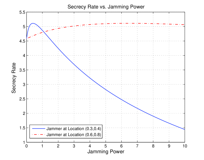
Figure 4: Secrecy rate vs. jamming power

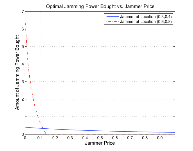
Figure 5: How much jamming power the sources buy as a function of the jammer price

For the single-jammer case, we consider two jammer locations which are $(0.3,0.4)$ and $(0.6,0.8)$. Fig. 4 shows the secrecy rate as a function of the jamming power when $p_{1}$, $p_{2}$, and $p_{r}$ are all set up to ${p_{max}}$. We can see that with the increase of the jamming power, the secrecy rate first increases and then decreases. There indeed exists an optimal point for the jamming power. Also the optimal point depends on the location of the friendly jammer, and we can find that the friendly jammer close to the malicious relay is more effective to improve the secrecy rate. Fig. 5 shows that the optimal amount of the jamming power bought by the sources depends on the price requested by the friendly jammer. We can see that the amount of bought power gets reduced if the price goes high and the sources would even stop buying after some price point. And thus there is a tradeoff for the jammers to set the price. If the price is set too high, the sources would buy less power or even stop buying.

For the multiple-jammer case, we consider two jammers which are located at $(0.3,0.4)$ and $(0.5,0.5)$, respectively. Note that in the simulations of this scenario the jammers are both sufficiently-effective ones. Here we define jammer $i$ as a sufficiently-effective one if it on its own can offer a power $p_{i}^{J}$, $p_{i}^{J}\in\left({0,{p_{max}}}\right]$, making the secrecy rate improved up to the maximal value. In Fig. 6, Fig. 7, Fig. 8, and Fig. 9, the secrecy rate $C_{s}$, the sources’ utility $U_{s}$, the first jammer’s utility $U_{1}$, and the second jammer’s utility $U_{2}$ as functions of both jammers’ prices are shown, respectively. In Fig. 6, we can see that there exists an upper bound and a lower bound for the secrecy rate when the channel conditions are settled. When one of the two jammers’ prices is low enough, the sources could buy sufficient jamming power from the jammer to improve the secrecy rate up to the upper bound. When both jammers’ prices are beyond the sources’ payment ability, the secrecy rate would stay at the lower bound which is the same as the case without jammers as the sources no longer buy jamming power from the jammers. In Fig. 7, we can see that if at least one of the two jammers sets a low price, the sources’ utility is high as the sources could get a high secrecy rate at a low cost from the jammer with low asking price. With both jammers’ prices going high, the sources’ utility decreases. When the prices of both jammers are so high that the sources cannot benefit any more from the jamming service at the high cost, the sources would stop buying. In Fig. 8 and Fig. 9, we can find that under this condition (i.e., both of the jammers are sufficiently-effective ones) the sources would always prefer to buying service from only one of the friendly jammers for the best performance. The selected jammer is either more effective to improve the secrecy rate when the prices of the jammers are comparable, or the one whose asking price is low enough. For the friendly jammer side, if the jammer asks too low price, the jammer’s utility is very low. But if the jammer asks too high price, the sources might buy the service from the other friendly jammer. Therefore, there is an optimal price for each friendly jammer to ask, and the sources would always select the one which can provide the best performance improvement.

For the multiple-jammer case, we also discuss how the optimal secrecy rate changes with the number of jammers increasing. We conduct simulations under two different scenarios, i.e., there exists at least one sufficiently-effective jammer and there is no sufficiently-effective jammer. Here no sufficiently-effective jammer means that the sources could not achieve the maximal secrecy rate with only one jammer’s help. Therefore, the sources have to first sort the current friendly jammers in an order of effectiveness, and then buy jamming power from the most effective jammer one by one until the secrecy rate reaches the maximal value. From (IV-A) and (IV-A), we can get that if the channel information and the transmitting power of the sources and the relay are settled, the maximal achievable secrecy rate will not change, no matter how many jammers are used and how much jamming power bought by the sources from each jammer. For the non-sufficiently-effective jammer scenario, we set the jammer $i$ located at $(x_{i},y_{i})$, $i\in\mathcal{N}$, where $x_{i}^{2}+y_{i}^{2}>4$. In Fig. 10, the optimal secrecy rate as a function of number of friendly jammers is shown. We can see that if there exists sufficiently-effective jammers, the optimal secrecy rate does not change as the number of jammers increases. For the sources, they always choose the most effective jammer to achieve the maximal secrecy rate, when additional jamming power from other jammers would decrease the optimal secrecy rate. In other words, in this scenario, the optimal secrecy rate can reach the maximal value with the most effective jammer’s help only. On the other hand, if there are no sufficiently-effective jammers, the optimal secrecy rate will be improved up to the maximal value as the number of jammers increases.

Finally, we compare the distributed solution with the centralized solution of secrecy rate. In Fig. 11, we show the optimal secrecy rate of both the distributed and centralized schemes as a function of the gain factor $a$ in (31) with the friendly jammer located at $(1,1)$. When $a$ is large, the sources would care the gain of secrecy rate more than the jamming service cost in the game theoretical scheme. We can see that the performance gap between the distributed and centralized solutions of optimal secrecy rate is shrinking as $a$ is increasing. And the solutions are asymptotically the same when $a$ is sufficiently large.

VI Conclusions

In this paper, we have investigated the physical layer security for two-way relay communications with untrusted relay and friendly jammers. As a simple case, a two-way relay system without jammers is first studied, and an optimal power allocation vector of the sources and relay nodes is found. We then investigated the secrecy rate in the presence of friendly jammers. Furthermore, we defined and analyzed a Stackelberg type of game between the sources and the friendly jammers to achieve the optimal secrecy rate in a distributed way. Finally, we obtained a distributed solution for the proposed game. From the simulation results we can get the following conclusions. First, a non-zero secrecy rate for two-way relay channel is indeed available. Second, the secrecy rate can be improved with the help of friendly jammers, and there is an optimal solution of jamming power allocation. Third, there is also a tradeoff for the price a jammer sets, and if the price is too high, the sources will turn to buying from others. For the game, we can see that the distributed algorithm and the centralized scheme have similar performances, especially when the gain factor is sufficiently large.

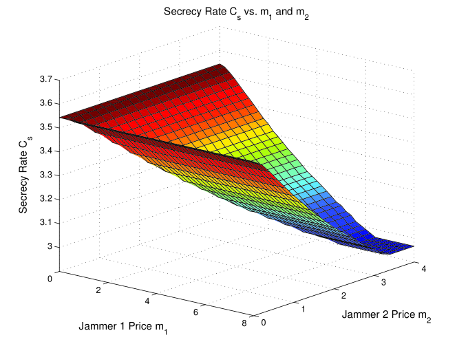
Figure 6: Secrecy rate $C_{s}$ vs. the prices of both jammers

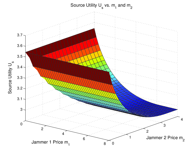
Figure 7: The sources’ utility $U_{s}$ vs. the prices of both jammers

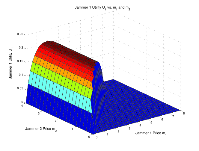
Figure 8: The jammer 1’s utility $U_{1}$ vs. the prices of both jammers

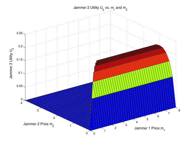
Figure 9: The jammer 2’s utility $U_{2}$ vs. the prices of both jammers

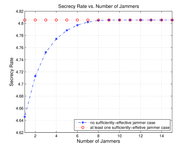
Figure 10: Secrecy rate vs. number of jammers

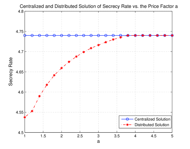
Figure 11: Centralized and distributed solution of secrecy rate vs. the gain factor

References

- [1] A. D. Wyner, “The wire-tap channel,” Bell System Technical Journal, vol. 54, no. 8, pp. 1355–1387, Oct. 1975.
- [2] S. K. Leung-Yan-Cheong and M. E. Hellman, “The Gaussian wiretap channel,” IEEE Transactions on Information Theory, vol. 24, no. 4, pp. 451–456, Jul. 1978.
- [3] I. Csiszár and J. Körner, “Broadcast channels with confidential messages,” IEEE Transactions on Information Theory, vol. 24, no. 3, pp. 339–348, May 1978.
- [4] P. Parada and R. Blahut, “Secrecy capacity of SIMO and slow fading channels,” in Proceedings of IEEE International Symposium on Information Theory, Adelaide, Australia, Sep. 2005.
- [5] J. Barros and M. R. D. Rodrigues, “Secrecy capacity of wireless channels,” in Proceedings of IEEE International Symposium on Information Theory, Seattle, USA, Jul. 2006.
- [6] Y. Liang, H. V. Poor, and S. Shamai (Shitz), “Secure communication over fading channels,” IEEE Transactions on Information Theory, vol. 54, no. 6, pp. 2470–2492, Jun. 2008.
- [7] P. K. Gopala, L. Lai, and H. E. Gamal, “On the secrecy capacity of fading channels,” IEEE Transactions on Information Theory, vol. 54, no. 10, pp. 4687–4698, Oct. 2008.
- [8] R. Negi and S. Goel, “Secret comunication using artificial noise,” in Proceedings of IEEE Vehicular Technology Conference, Dallas, Texas, USA, Sep. 2005.
- [9] S. Shafiee and S. Ulukus, “Achievable rates in Gaussian MISO channels with secrecy constraints,” in Proceedings of IEEE International Symposium on Information Theory, Nice, France, Jun. 2007.
- [10] A. Khisti, G. Wornell, A. Wiesel, and Y. Eldar, “On the Gaussian MIMO wiretap channel,” in Proceedings of IEEE International Symposium on Information Theory, Nice, France, Jun. 2007.
- [11] F. Oggier and B. Hassibi, “The secrecy capacity of the MIMO wiretap channel,” in Proceedings of IEEE International Symposium on Information Theory, Toronto, Canada, Jul. 2008.
- [12] S. Shafiee, N. Liu, and S. Ulukus, “Towards the secrecy capacity of the Gaussian MIMO wire-tap channel: The 2-2-1 channel,” IEEE Transactions on Information Theory, vol. 55, no. 9, pp. 4033–4039, Sep. 2009.
- [13] Y. Liang and H. V. Poor, “Generalized multiple access channels with confidential messages,” in Proceedings of IEEE International Symposium on Information Theory, Seattle, USA, Jul. 2006.
- [14] Y. Liang and H. V. Poor, “Multiple-access channels with confidential messages,” IEEE Transactions on Information Theory, vol. 54, no. 3, pp. 976–1002, Mar. 2008.
- [15] I. Csiszár and P. Narayan, “Secrecy capacities for multiterminal channel models,” IEEE Transactions on Information Theory, vol. 54, no. 6, pp. 2437–2452, Jun. 2008.
- [16] A. Khisti, A. Tchamkerten, and G. W. Wornell, “Secure broadcasting over fading channels,” IEEE Transactions on Information Theory, vol. 54, no. 6, pp. 2453–2469, Jun. 2008.
- [17] E. Tekin and A. Yener, “The general Gaussian multiple-access and two-way wiretap channels: Achievable rates and cooperative jamming,” IEEE Transactions on Information Theory, vol. 54, no. 6, pp. 2735–2751, Jun. 2008.
- [18] R. Liu, T. Liu, H. V. Poor, and S. Shamai (Shitz), “MIMO Gaussian broadcast channels with confidential messages,” in Proceedings of IEEE International Symposium on Information Theory, Seoul, Korea, Jul. 2009.
- [19] L. Dong, Z. Han, A. P. Petropulu, and H. V. Poor, “Secure wireless communications via cooperation,” in Proceedings of 46th Annual Allerton Conference on Communication, Control, and Computing, UIUC, Illinois, USA, Sep. 2008.
- [20] L. Dong, Z. Han, A. P. Petropulu, and H. V. Poor, “Amplify-and-forward based cooperation for secure wireless communications,” in Proceedings of IEEE International Conference on Acoustics, Speech, and Signal Processing, Taipei, Taiwan, Apr. 2009.
- [21] L. Dong, Z. Han, A. P. Petropulu, and H. V. Poor, “Improving wireless physical layer security via cooperating relays,” IEEE Transactions on Signal Processing, vol. 58, no. 3, pp. 1875–1888, Mar. 2010.
- [22] L. Lai and H. E. Gamal, “The relay-eavesdropper channel: Cooperation for secrecy,” IEEE Transactions on Information Theory, vol. 54, no. 9, pp. 4005–4019, Sep. 2008.
- [23] Y. Oohama, “Coding for relay channels with confidential messages,” in Proceedings of IEEE Information Theory Workshop, Cairns, Australia, Sep. 2001.
- [24] Y. Oohama, “Capacity theorems for relay channels with confidential messages,” in Proceedings of IEEE International Symposium on Information Theory, Nice, France, Jun. 2007.
- [25] X. He and A. Yener, “Cooperation with an untrusted relay: A secrecy perspective,” IEEE Transactions on Information Theory, vol. 56, no. 8, pp. 3807–3827, Aug. 2010.
- [26] X. He and A. Yener, “Two-hop secure communication using an untrusted relay: A case for cooperative jamming,” in Proceedings of IEEE Global Telecommunications Coference, New Orleans, LA, USA, Dec. 2008.
- [27] B. Rankov and A. Wittneben, “Achievable rate regions for the two-way relay channel,” in Proceedings of IEEE International Symposium on Information Theory, Seattle, USA, Jul. 2006.
- [28] B. Rankov and A. Wittneben, “Spectral efficient protocols for half-duplex fading relay channels,” IEEE Journal on Selected Areas in Communications, vol. 25, no. 2, pp. 379–389, Feb. 2007.
- [29] T. Cui, T. Ho, and J. Kliewer, “Memoryless relay strategies for two-way relay channels,” IEEE Transactions on Communications, vol. 57, no. 10, pp. 3132–3143, Oct. 2009.
- [30] R. Zhang, Y. C. Liang, C. C. Chai, and S. Cui, “Optimal beamforming for two-way relay channel with analogue network coding,” IEEE Journal on Selected Areas in Communications, vol. 27, no. 5, pp. 699–712, Jun. 2009.
- [31] C. Hausl and J. Hagenauer, “Iterative network and channel decoding for the two-way relay channel,” in Proceedings of IEEE International Conference on Communications, Istanbul, Turkey, Jun. 2006.
- [32] D. Fudenberg and J. Tirole, Game Theory, MIT Press, Cambridge, MA, 1993.
- [33] Z. Han, D. Niyato, W. Saad, T. Basar, and A. Hjørungnes, Game Theory in Wireless and Communication Networks: Theory, Models and Applications, in print, Cambridge University Press, UK, 2010.
- [34] J. Huang, D. P. Palomar, N. B. Mandayam, S. B. Wicker, J. Walrand, and T. Basar, “Game theory in communication systems,” IEEE Journal on Selected Areas in Communications, vol. 26, no. 7, Sep. 2008.
- [35] E. A. Jorswieck, E. G. Larsson, M. Luise, and H. V. Poor, “Game theory in signal processing and communications,” IEEE Signal Processing Magazine, vol. 26, no. 5, Sep. 2009.
- [36] Z. Han, N. Marina, M. Debbah, and A. Hjørungnes, “Physical layer security game: Interaction between source, eavesdropper and friendly jammer,” EURASIP Journal on Wireless Communications and Networking, Jun. 2009.
- [37] Z. Han, N. Marina, M. Debbah, and A. Hjørungnes, “Physical layer security game: How to date a girl with her boyfriend on the same table,” in Proceedings of IEEE International Conference on Game Theory for Networks, Istanbul, Turkey, May 2009.
- [38] S. Verdú, Multiuser Detection, Cambridge University Press, UK, 1998.
- [39] G. Papavassilopoulos and J. Cruz, “Nonclassical control problems and Stackelberg games,” IEEE Transactions on Automatic Control, vol. 24, no. 2, pp. 155–166, Apr. 1979.
- [40] Z. Han and K. J. R. Liu, Resource Allocation for Wireless Networks: Basics, Techniques, and Applications, Cambridge University Press, UK, 2008.
- [41] R. Yates, “A framework for uplink power control in cellular radio systems ,” IEEE Journal on Selected Areas in Communications, vol. 13, no. 7, pp. 1341–1348, Sep. 1995.
- [42] N. Bonneau, M. Debbah, E. Altman, and A. Hjørungnes, “Non-atomic games for multi-user systems,” IEEE Journal on Selected Areas in Communications, vol. 26, no. 7, pp. 1047–1058, Sep. 2008.
- [43] S. Boyd and L. Vandenberghe, Convex Optimization, Cambridge University Press, UK, 2006.
- [44] M.-K. Oh, X. Ma, G. Giannakis, and D.-J. Park, “Cooperative syynchronization and channel estimation in wireless sensor networks,” in Proc. 37th Asilomar Conf. Signals, Systems and Computers, Nov. 2003.
- [45] Q. Huang, M. Ghogho, J. Wei, and P. Ciblat, “Practical timing and frequency synchronization for OFDM-based cooperative systems,” IEEE Transaction on Signal Processing, vol. 58, no. 7, Jul. 2010.