A Hierachical Evolutionary Algorithm for Multiobjective Optimization in IMRT

Abstract

Purpose: Current inverse planning methods for IMRT are limited because they are not designed to explore the trade-offs between the competing objectives between the tumor and normal tissues. Our goal was to develop an efficient multiobjective optimization algorithm that was flexible enough to handle any form of objective function and that resulted in a set of Pareto optimal plans.
Methods: We developed a hierarchical evolutionary multiobjective algorithm designed to quickly generate a small diverse Pareto optimal set of intensity modulated radiation therapy (IMRT) plans that meet all clinical constraints and reflect the optimal trade-offs in any radiation therapy plan. The top level of the hierarchical algorithm is a multiobjective evolutionary algorithm (MOEA). The genes of the individuals generated in the MOEA are the parameters that define the penalty function minimized during an accelerated deterministic IMRT optimization that represents the bottom level of the hierarchy. The MOEA incorporates clinical criteria to restrict the search space through protocol objectives and then uses Pareto optimality among the fitness objectives to select individuals. The population size is not fixed, but a specialized niche effect, domination advantage, is used which controls the patient size and plan diversity. The number of fitness objectives is kept to a minimum for greater selective pressure, but the number of genes is expanded for flexibility that allows a better approximation of the Pareto front.
Results: Acceleration techniques implemented on both levels of the hierarchical algorithm resulted in short, practical runtimes for multiobjective optimizations. The MOEA improvements were evaluated for example prostate cases with one target and two OARs. The modified MOEA dominated 11.3% $\pm$ 0.7% of plans using a standard genetic algorithm package. By implementing domination advantage and protocol objectives, small and diverse populations of clinically acceptable plans that were only dominated 0.2% $\pm$ 0.05% by the Pareto front could be generated in a fraction of an hour.
Conclusions: Our MOEA produces a diverse Pareto optimal set of plans that meet all dosimetric protocol criteria in a feasible amount of time. Our final goal is to improve practical aspects of the algorithm and integrate it with a decision analysis or human interface for selection of the IMRT plan with the best possible balance of successful treatment of the target with low OAR dose and low risk of complication for any specific patient situation.

Keywords:
multiobjective optimization, evolutionary algorithm, radiation oncology, IMRT

1 Introduction

Intensity modulated radiation therapy (IMRT) uses inverse planning optimization to determine complex radiation beam configurations that will deliver dose distributions to the patient that are better than could be achieved using 3D conformal radiation therapy. The problem is inherently multiobjective with competing clinical goals for a high, uniform target dose and low dose to the organs at risk (OAR). The IMRT inverse planning algorithms commonly optimize a single objective function (also known as ”penalty function”) that is a linear combination of many separate organ and tumor-specific objective (penalty) functions. The solution of this problem is one point in the space of feasible treatment plans. To find another point in this space, the user can vary any one of the parameters that make up the penalty function. Current clinical algorithms do not provide methods for efficiently searching this space of feasible plans. The search is complicated by the fact that in comparing plans, one plan may have achieved superior values for some objectives but inferior values for other objectives.

A multiobjective optimization (MOO) algorithm is one method for searching through the space of feasible plans. Such an algorithm varies the parameters that define an objective function and calculates a new plan for each new function. For each plan created, the algorithm calculates objective values that characterize its quality. If all of the objective values of one plan are better or the same as the values of a second plan, the first plan is said to dominate the second. A plan is said to be Pareto optimal if there are no plans that dominate it. Note that any Pareto optimal plan has some superior objective values compared to other Pareto optimal plans, but inferior values for others. MOO algorithms must generate a large number of plans that each require an individual IMRT optimization. The resulting computation time could make this algorithm impractical depending on the efficiency of IMRT optimization method used and the number of plans required. The final product of a MOO algorithm is a set of Pareto optimal plans, known as the Pareto front, so ultimately, there must be a method to select the individual plan to be used.

The true Pareto front of this multiobjective problem is a multidimensional surface that contains an infinite number of points, and hence there is the potential for the production of Pareto populations that are too large for practical purposes. Methods for handling this issue, called niche functions, come in many forms, but are all designed to limit the number of individuals that can survive in a population while maintaining diversity. For stochastic multiobjective algorithms to be practical, the use of an appropriate niche function may be quite important.

The nature of the separate objective functions used in the MOO plays an important role in the optimization. Those functions that are convex may be optimized using deterministic algorithms. Stochastic optimization methods are needed for optimizing those functions that are not convex to avoid becoming trapped in local minima. In selecting a multiobjective optimization approach, the user may have to make a decision between using a deterministic method that is fast but limits the type of objectives and a stochastic method that is very flexible but slower. If different objective functions are used to evalute the quality of dose distributions than are used in the single penalty function that optimizes beamlet intensities, it is possible that some parts of the optimization can be done deterministically while other parts may use stochastic methods.

One type of stochastic optimization algorithm is an evolutionary algorithm which uses concepts based on genetics and natural selection to create a population of new solutions and to select the fittest among them. An ”individual” is described by a set of genes. New individuals are created through recombination of genes from two ”parent” individuals selected from the existing population. Random mutations can occur which help prevent the population from becoming trapped in local minima. Natural selection of superior individuals followed by reproduction using their genes leads the algorithm to find the Pareto optimal solutions. In practice, further heuristic methods are often needed to speed up this process.

This paper describes the development of a multiobjective optimization algorithm that combines an evolutionary method to search feasible plan space with a deterministic method using a single objective penalty function that quickly finds the optimal beamlet intensities for that function. While the penalty function must be convex, the hierarchical method allows us to use any fitness objective (convex or non-convex) to evalute plan quality without losing too much in speed. Utilization of a MOO algorithm requires the selection of one plan from the Pareto optimal set to be used for IMRT treatment of the patient. There are many methods for doing so. We have selected an a posteriori method of multiobjective optimization where plan selection is done after the Pareto front is found by either an influence diagram [1, 2] or inspection by a radiation oncologist. With both of these approaches, it is best to restrict the set of plans to a relatively small number, e.g. 10-20, and this is reflected in our MOO algorithm.

In the methods section, the hierarchical algorithm is described with the emphasis on the evolutionary element and how it interacts with the deterministic step. In the results, performance of the algorithm is characterized using two clinical prostate cancer cases.

2 Methods and Materials

A multiobjective evolutionary algorithm (MOEA) has been developed for the top level of a hierarchical IMRT optimization method. The lower level is a deterministic algorithm that incorporates a constrained quadratic optimization algorithm (BOXCQP). We have used a hierarchical process because there are two sets of variables we would like to optimize: (1) beamlet intensities (deterministic optimization), and (2) the objective parameters such as maximum dose, dose homegeneity, etc (stochastic optimization). At the stochastic level of the algorithm, an individual is created and each individual is characterized by a set of genes that determine the relative weighting between OARs and targets and a set of genes that describe the OAR penalty functions. The deterministic algorithm incorporates these genes into a quadratic objective function which is then solved for the beamlet intensities. The MOEA uses a separate set of objectives to determine the quality of each individual treatment plan. As mentioned above, considerations of speed have led us to incorporate several heuristic stages in our algorithm which results in a faster convergence to a clinically-acceptable set of Pareto optimal plans.

The following sections provide more detail of the algorithm as well as descriptions of the methods used to characterize the performance of the MOEA.

2.1 Multiobjective Evolutionary Algorithm

An evolutionary algorithm was chosen as the stochastic component of the multiobjective method because of its effectiveness in searching large regions of solution space while still incorporating techniques for focusing the search on regions more likely to produce better plans [3, 4, 5, 6, 7]. A number of characteristics of the IMRT optimization problem guided the development of our MOEA. The critical factors were (1) the very large search space, (2) the relatively large number of objectives, (3) the need for solutions to conform to ”clinically-acceptable” criteria, and (4) the time constraints for clinical use. In short, our modified MOEA was designed for faster and more effective convergence to the Pareto front inside the clinically acceptable space. The elements of the MOEA and highlights of the impact of these critical factors are described below.

2.1.1 Enhancements to the MOEA

Our MOEA uses no fixed number of individuals per generation, no summary single fitness function, and no tournament style selection method (as are common in traditional genetic algorithms). Instead, individuals are created one at a time and are eliminated if they are Pareto dominated by any existing individual or if they violate any clinical constraints. Conversely, if the new individual dominates any of the current population, those dominated individuals will be eliminated. If the individual survives, its genes become candidates for recombination in the next individual. In addition to these algorithmic modifications, various parameters of the multiobjective method, such as mutation rate, have been optimized for performance.

We also implemented a specialized niche function, called domination advantage. When calculating whether plan A dominates plan B, each objective value of plan A only needs to be within an $\epsilon$ of the corresponding plan B objective in order to dominate it. This domination advantage, $\epsilon$, can be thought of as the difference in objective values below which the clinical significance cannot be determined. Thus, it provided a means to avoid clustering of solutions so that the Pareto optimal set spans the entire clinically relevant space. It was also used to limit the total number of plans. The $\epsilon$ used in domination advantage was not a constant but was set equal to $c\cdot(n_{current}-n_{goal})$. The constant $c$ was adjusted so that the final number of plans was approximately the desired number, $n_{current}~{}\sim~{}n_{goal}$.

If two individuals were being compared to test for domination and were very close together, i.e. with all objective values within $\epsilon$ of each other, both individuals would ’dominate’ the other using domination advantage. In this rare case, a single fitness function was used that was a weighted sum of fitness objectives using importance weighting predetermined by the user. The individual with the worse single fitness function would be eliminated and the other would survive. Note that the result is different from might occur in traditional evolutionary algorithms where two individuals from different regions of the objective space would be forced into such a comparison. In our algorithm, these two individuals are so close together, the assumption is that little information of clinical value would be lost by the undesirable, but necessary, use of a single fitness function elimination.

We used two sets of objectives in the stochastic part of the algorithm, which we call fitness objectives and protocol objectives. Fitness objectives are the dosimetric functions that best represent the clinical goals and are used to determined plan quality. Protocol objectives are functions that delineate certain dosimetric cutpoints that need to be met, usually because of clinical protocol restrictions. Protocol objectives will restrict the search space such that the final set of plans are guaranteed to meet all clinical criteria. As will be described in more detail below, these two sets of objective functions are distinct and play different roles during the optimization.

2.1.2 Fitness and Protocol Objectives

In multiobjective optimization, smaller numbers of fitness objectives tend to result in greater selective pressure and better performance. Thus, it is desirable to have only one fitness objective for each structure. We chose effective uniform dose (EUD) as an appropriate objective for OARs; other functions such as complication probability functions could also be used. Unlike for OARs, we did not find target EUD to be an effective objective, because a uniform target at prescription dose could be deemed equivalent to a dose distribution with high variance and a higher mean dose. Typically, target dose distributions must meet minimum dose requirements as well as limits on inhomogeneity. We removed the minimum dose objective by prioritizing it and scaling the dose distributions to meet all minimum dose requirements, thereby leaving maximum dose (dose homogeneity) as the sole target objective.

The two sets of objective functions that were used are:

• Fitness objectives
  

  $$\begin{split}\vec{f}_{fit}(\vec{x})&=(f_{fit,1}(\vec{x}),\cdots,f_{fit,m}(\vec{x}),f_{fit,m+1}(\vec{x}),\mathellipsis,f_{fit,m+n}(\vec{x})),\\ \text{where}~{}m&=\#~{}\text{of target fitness objectives}\\ n&=\#~{}\text{of OAR fitness objectives}\\ f_{fit,i}(\vec{x})&=d^{max}_{i}\text{ for}~{}i\in\{1,\mathellipsis,m\}\text{, i.e. for targets}\\ f_{fit,i}(\vec{x})&=~{}EUD(\vec{d})~{}=~{}(1/nvox_{i}\sum\limits_{j=1}^{nvox_{i}}d_{j}^{a_{i}})^{1/a_{i}}~{}\text{for}~{}i~{}\in~{}\{m+1,\mathellipsis,m+n\}\text{, i.e. for OARs}.\\ \end{split}$$ (1)

  where $d_{j}$ is the dose to $j^{th}$ OAR voxel, $nvox_{i}$ is the number of voxels in the $i^{th}$ OAR, $d^{max}_{i}$ is the maximum dose to any voxel within the ith target, and $a_{i}$ is a constant ($>$ 1) that characterizes the radiation response of each of the $n$ OARs [8, 9, 10].

• Protocol objectives
  

  $$\begin{split}\vec{f}_{prot}(\vec{x})&=(f_{prot,1}(\vec{x}),\cdots,f_{prot,p}(\vec{x}),f_{prot,p+1}(\vec{x}),\mathellipsis,f_{prot,p+q}(\vec{x})),\\ \text{where}~{}p&=\#~{}\text{of target protocol objectives}\\ q&=\#~{}\text{of OAR protocol objectives}\\ f_{prot,k}&~{}=~{}\begin{cases}d^{max}_{k}&\text{if}~{}d^{max}_{k}>D_{prot,k}\\ 0&\text{otherwise}\end{cases}~{}\text{ for all clinical maximum dose contraints}\\ f_{prot,k}&~{}=~{}\begin{cases}nvox_{violate,k}&\text{if}~{}\frac{nvox_{violate,k}}{nvox_{k}}>V_{OAR,k}\\ 0&\text{otherwise}\end{cases}~{}\text{ for all clinical dose volume constraints}\\ \end{split}$$ (2)

  where $D_{prot,k}$ is the maximum dose allowed allow to the structure associated with the $k^{th}$ protocol objective, $nvox_{violate,k}$ is the number of voxels in the OAR associated with the $k^{th}$ protocol objective that receive doses that exceed the allowed dose of a dose volume constraint (DVC), $nvox_{k}$ is the total number of voxels in the OAR associated with the $k^{th}$ protocol objective, and $V_{OAR,k}$ is the maximum fraction of the OAR associated with the $k^{th}$ protocol objective allowed over the dose for a DVC. Minimum target dose constraints are achieved by scaling the dose distribution if necessary.

2.1.3 Stages of the MOEA

There are three stages of the MOEA that correspond to: (1) a broad search of the feasible plan space, (2) a focusing of the search to a region of space that meets protocol requirements and (3) a search of the feasible space within the protocol constraints. Throughout the last two stages, the domination advantage procedure is used to both spread the plans out (avoiding clustering near local minima) and to limit the number of plans. As the optimization proceeds, the current set of solutions approaches the true Pareto front defined by the fitness objectives.

In stage 1, the individuals were created by random selection of genes. The genes were used to construct the quadratic objectives of the deterministic part of the algorithm (see Sec. 2.2). Then the fitness and protocol objective values were calculated, and the individual was added to or rejected from the current population, whose size was $n_{current}$. When $n_{current}$ equaled the pre-defined number of desired plans determined by the decision procedure, $n_{goal}$, stage 1 ended.

In stage 2, new individuals were created by recombination of current genes and mutation. During this stage, the direction of mutations were guided depending on whether or not the parent plan met the protocol objectives in order to more quickly search relevant space. Selection proceeded as in stage 1 with the addition of the domination advantage procedure. In this stage, the population was allowed to grow larger than $n_{goal}$. Stage 2 ended when there were $n_{goal}$ individuals who met all of the clinical criteria (protocol objective values = 0), at which time, all individuals who did not meet these objectives were eliminated.

Stage 3 proceeded similarly as stage 2 except that the protocol objectives were converted to constraints, mutation direction was not guided, and Pareto optimality was determined only by the fitness objectives. This stage ran for a pre-determined number of iterations.

One reason to separate the objectives into two sets is to reduce the dimensionality of the final solution space. As the number of fitness objectives considered in Pareto domination increases, the probability of domination is reduced by a factor on the order of $\sim.5^{n_{objectives}}$, and hence selective pressure was reduced. By converting protocol objectives into constraints, the solution space was restricted to a smaller number of dimensions equal to the smaller number of fitness objectives.

A multiobjective optimization algorithm needs to be paired with a decision making component. This will have an impact on the number and variation of the solution set. In our case, the decision maker is either a human or an influence diagram, neither of which can handle large numbers of solutions or very nearly identical solutions. Hence, our algorithm was designed to produce on the order of $n_{goal}$ plans, i.e. 10-15 plans for $n_{goal}$ = 10. The algorithm can be adjusted to produce any size solution set.

2.2 Deterministic Algorithm

For the beamlet intensity optimization, we employed a modification of the Bound Constrained Convex Quadratic Problem (BOXCQP) algorithm [11, 12, 13]. This efficient method was implemented to minimumize a quadratic objective function with the bound constraint that all beamlet intensities are non-negative and less then some maximum allowed beamlet intensity, $x_{max}$. Non-zero penalty factors were assigned to OAR voxels that had exceeded the OAR dose parameter in each iteration. A short description is provided.

To compute optimal beamlet intensities, BOXCQP minimized the matrix form of the penalty function defined by each individual’s genes summed with a smoothing function as described below:

$$\begin{split}\mbox{minimize }~{}f_{det}(\vec{x})&\medspace=(\vec{d}-\vec{D}_{det})^{T}P(\vec{d}-\vec{D}_{det})|_{\vec{d}=B\cdot\vec{x}}\\ &\qquad+~{}\kappa(S\vec{x})^{T}(S\vec{x})\\ &\mbox{ subject to }0\leq x_{b}\leq x_{max}\\ \end{split}$$ (3)

where $f_{det}$ is the objective function for the determinstic component of the algorithm, $\vec{x}$ is the vector of the beamlet intensities, $B$ is the precalculated matrix storing the dose to each voxel from each beamlet, $P$ is a diagonal matrix of all importance weighted penalty factors for each voxel, $\kappa$ is the smoothing constant, S is the smoothing penalty matrix, and $x_{b}$ represents any element in vector $\vec{x}$

A smoothing term was introduced because BOXCQP depends on solving a well-posed problem [11, 12]. It is also desirable to find the deliverable solution for a beamlet weight vector $\vec{x}$ that is not excessively modulated due to delivery limitations, i.e. MLC movement. The smoothing term was based on the fact that the smaller the second derivative of a fluence map, the easier it is to deliver in practice. Therefore, $S$ was the second derivative matrix by finite difference method, and $\kappa$ was a smoothing coefficient that was found empirically.

The algorithm was implemented using Matlab. Since this code was executed many times during the course of the optimization, considerable effort was taken to speed execution.

2.3 Treatment planning platform

A treatment plan consists of a set of beams, which describe the geometry of radiation delivery. Each radiation beam was divided into a 2D array of beamlets. Each beamlet represents a .6 cm by 1 cm area of the beam. A beamlet length of 1 cm was selected because of the size of the collimator leaf, and a width of 0.6 cm was used as a compromise between speed and resolution. Beamlet intensities were the variables optimized in the deterministic IMRT optimization algorithm.

The patient was considered as a collection of 3D voxels that are segmented into a set of targets and critical normal tissues (OARs). A model of radiation transport mapped each beamlet intensity to the dose it deposited at each voxel; this was stored in a beamlet-to-voxel dose contribution matrix, which was calculated once before the optimization. Typically the number of beamlets ranged from 1000-5000 while the number of voxels ranged from 10⁴ to 10⁵. The entire system was modeled using the Prism treatment planning system [14, 15, 16] that was augmented with a pencil beam dose calculation algorithm [17]. The optimization algorithms interacted with Prism via file input/output.

2.4 Experiments

As the focus of this work is to introduce this multiobjective method, results are shown for only two prostate cancer example cases. Case 1, used in all experiments, was selected to be challenging and had a PTV that was $\sim$8.5 cm across at the widest point and had 39% overlap with the bladder and 32% overlap with the rectum. Case 2, used only in sections 3.5 and 3.6, had a PTV that was $\sim$7cm in diameter with only 9% overlap with the bladder and 17% overlap with the rectum. All plans used seven equally spaced 6 MV photon beams.

Three fitness objectives were used in all of the optimizations: bladder (or bladder wall) EUD, rectal wall EUD, and target maximum dose. OAR voxels inside the PTV were excluded from objective calculation. All dose distributions were scaled to meet minimum target dose requirements, thereby making the target maximum dose a measure of target variance. The protocol objectives represented a maximum allowed target dose and OAR DVH constraints. A comparison was also made for two example prostate patients between the MOEA and a plan generated using a commercial objective deterministic IMRT optimization algorithm with the current clinical protocol. Of all possible MOEA plans, we chose the one plan from the MOEA output that most closely matched the clinical plan’s target dose distribution.

It should be noted that stochastic algorithms do not guarantee convergence to the Pareto optimal set. The degree to which this algorithm approximates that set is the subject of several of the result sections described below.

The following experiments were performed to evaluate individual aspects of the algorithm:

• demonstration of the evolution of a population of IMRT plans towards the Pareto front through the three stages of a multiobjective optimization (Section 3.1);

• a mulitobjective comparison of performance between a standard genetic algorithm package and the modified evolutionary algorithm (Section 3.2);

• demonstration of the role of domination advantage in controlling population size, maintaining diversity, and improving performance (Section 3.3);

• evaluation of the performance of the MOEA with and without protocol objectives (Section 3.4);

• a DVH comparison between plans produced by the MOEA and plans produced using our current clinical protocol and a commercial planning system (Section 3.5);

• assessment of the ability of the MOEA to approximate the true Pareto front (Section 3.6).

A common method for comparing two different algorithms is to select the ’best’ plan from each population and do DVH comparisons; however, such a method is not a multiobjective metric that can compare algorithms that produce populations of plans. It focuses on only a small subset of the results, does not lead itself to quantitative or statistical analysis, and, given the multiobjective nature of the problem, selection of the plan used for comparison is subjective. As previously discussed, in multiobjective optimization a plan can only be deemed superior to another if it is better in all of its objectives, which is the definition of Pareto domination. In our evaluation of different multiobjective algorithms, we used a metric based on Pareto dominance that we term ”domination comparison”, $C_{D}$. This is the percentage of all possible comparisons between two groups of plans in which the plan from the first population dominates the plan from the second population. In mathematical form, the domination comparison metric for a population resulting from one algorithm, $U$, in comparison with a population of plans obtained with another algorithm, $V$, is defined as follows:

$$\begin{split}\text{Let the set of plans obtained by formulation}~{}U~{}&=~{}\vec{u}\\ \text{and those obtained by formulation}~{}V~{}&=~{}\vec{v}\\ \text{and}~{}C_{D}~{}=~{}\frac{\sum_{i}\sum_{j}f(u_{i},v_{j})}{|U|*|V|}\\ \text{ where}~{}f(u_{i},v_{j})=1\text{ if }~{}u_{i}\text{~{}dominates~{}}v_{j}\\ \text{and }f(u_{i},v_{j})=0~{}\text{otherwise.}~{}\\ \end{split}$$ (4)

Domination comparison is a purely multiobjective metric that gives some indication of which of two populations is closer to the Pareto front; however, it does not give a measure of the diversity of the population or coverage of the Pareto front. For this reason we included 3-D Pareto plots for graphical display of the final populations for the two prostate examples. For greater ease, we made all of these plots uniform, with rectum objective on the x-axis, bladder objective on the y-axis, and target objective in color scale.

3 Results

3.1 Stages of the MOEA

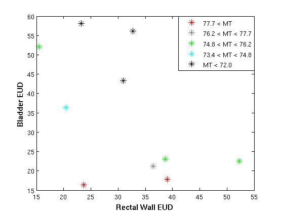
(a)

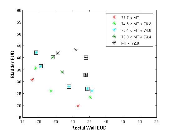
(b)

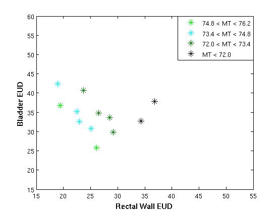
(c)

Figure 1: Plots of the objective values of the plans at the end of (a) stage 1, (b) stage 2, and (c) stage 3. The colors represent different values for the target objective, MT. In (b), the square icons represent plans that met the clinical protocol objectives.

A population of plans for case 1 was tracked through the three stages of the evolutionary algorithm (Figures 1a, 1b, and 1c). Three fitness objectives were used: rectal wall EUD, bladder EUD, and maximum target dose (MT). Only OAR voxels outside the target were used in the calculation of the fitness objectives.

Often Pareto optimality is demonstrated using only two objectives which makes determining the Pareto front visually easy. Given that we used three fitness objectives, we used color to indicate the value of the third axis. For uniformity, rectal wall EUD was plotted on the X-axis, bladder EUD on the Y-axs, and the value of the maximum target dose (MT) was represented in color scale. The plots illustrate the difficulty in visualizing even a 3-dimensional fitness objective space, which is small compared the the dimensions of most IMRT planning.

Dose distributions were scaled to meet all minimum target dose requirements to eliminate the need for a minimum target dose fitness objective. The maximum target dose represents clinically undesirable hot spots and is a measure of target variance. Throughout the presentations of these results, lower fitness objective values correspond to more optimal plans. We used $n_{goal}$ = 10 throughout this work.

The population after the first 10 iterations obtained from completely random genes have relatively poor objective values. Stage 2 is complete after 53 iterations, and objectives values have improved. The ten clinically acceptable plans are shown with a black box outline. All other plans were removed before stage 3 began. For this example, the greatest amount of improvement is seen in a small number of iterations during stage 2 as the initial population was not close to Pareto optimal. Stage 3 was completed after a total of 200 iterations. Further improvement is observed in the objective space during stage 3.

3.2 Performance of the Hierarchical Evolutionary Algorithm

The modified evolutionary algorithm was compared to the Matlab standard genetic algorithm package that used a single stage, a set population size, and used a tournament-style selection method with a single fitness function. Both algorithms used the previously described deterministic algorithm. To isolate differences in the algorithms, domination advantage and protocol objectives were not used in either multiobjective optimization. Important differences included the selection method, allowed population size, and mutation rates. Bladder EUD, rectal wall EUD and maximum target dose (MT) were used as the fitness objectives.

Twenty-five multiobjective optimizations that each produced a set of 11 to 15 plans were performed for both situations to establish statistical significance, and each multiobjective optimization executed a total of 200 BOXCQP iterations in $\sim$10 minutes. Objective values (OAR EUD and target maximum dose) for individual plans resulting from two optimizations are shown in Figure 2.

Populations resulting from our MOEA dominated populations resulting from the standard genetic algorithm $D_{C}$ = 11.3% $\pm$ 0.7% of possible comparisons versus $D_{C}$ = 0.04% $\pm$ 0.02% in reverse. Results indicate that the new evolutionary algorithm was able to produce a population of plans with lower OAR EUD values and lower target variance in a short amount of time.

3.3 Domination Advantage

Our MOEA does not have a set population size or limit and does not use a single-objective fitness function for selection. Resulting populations could potentially be very large even with a relatively small number of objectives. To keep the population size in the desired range, to increase selective pressure, and to promote diversity in the population, a specialized niche effect, domination advantage, was used. With domination advantage, once the population was greater than $n_{goal}$, potentially dominating individuals were given an advantage when testing for domination. One or more objectives of a dominating individual can be inferior as long as it was within $\epsilon$ of the objective of the individual being tested. The size of $\epsilon$ increased linearly with the difference between the $n_{current}$ and $n_{goal}$. A comparison of two multiobjective optimizations of a prostate case (with and without domination advantage) was performed to demonstrate the effect on a single population (Figure 3). Twenty-five multiobjective optimizations were performed with and without domination advantage to establish statistical significance.

Average population size without domination advantage was 68.7 $\pm$ 2.1 versus 13.2 $\pm$ 0.2 with domination advantage. The population generated using the niche effect dominated an average of $D_{C}$ = 1.73% $\pm$ 0.35% of the population generated without it and $D_{C}$ = 0.17% $\pm$ 0.04% of dominations occurred in reverse. In addition to creating a smaller, diverse population, improvement in the resulting population was observed when domination advantage was used. When domination advantage was used, there were fewer individuals for a more managable final population size, and individuals were closer to the true Pareto front possibly due to the increase in selective pressure from the niche effect. Domination advantage did not allow searching in regions that give only a small improvement in one objective at great cost to other objectives. This speeds up the optimization; however, it also means that some of the Pareto front may not be mapped.

3.4 Effect of Protocol Objectives

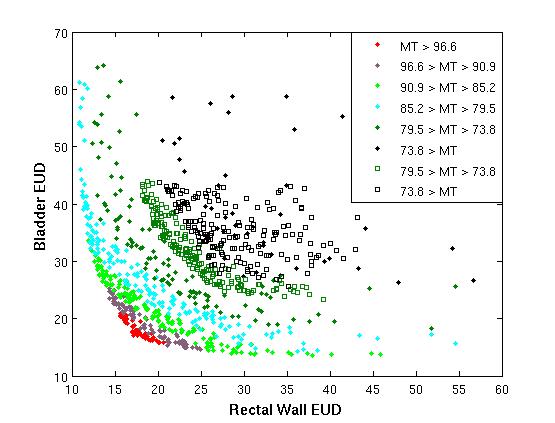
Figure 4: Plot comparing multiobjective optimization with (WP) and without (NP) using protocol objectives. Bladder EUD and Rectum EUD are plotted for the sum of 25 full optimizations with and without using protocol objectives to restrict the search space. Maximum target dose (MT), the target variance objective, is plotted in color. The solid circles show the full Pareto front, and the open squares display the optimizations using protocol objectives.

Protocol objectives were used to focus the search to a region of objective space that met pre-determined clinical dosimetric requirements. Performance of multiobjective optimizations were evaluted for an example prostate case with and without protocol objectives that reflected constraints from a clinical protocol. The effectiveness of the preference space guidance algorithm is shown in Figure 4.

In terms of Pareto domination the protocol objectives did not improve or degrade results; however, without protocol objectives, the search focused on too wide a search space. Of all individual plans generated without using protocol objectives, only 4.4% $\pm$ 0.8% met the clinical criteria, and only 68% of the full multiobjective optimizations had at least one plan that met all clinical requirements. In other words, 32% of the optimization procedures did not yield a usable plan when the protocol constraints were considered, whereas all of the plans generated using the protocol objectives met all of the clinical criteria.

3.5 Two Clinical DVH Comparisons

The MOEA was compared to our clinical planning methods for the two prostate cases. IMRT plans were optimized using a 200 iteration MOEA optimization and using our standard clinical inverse planning procedure. The MOEA plan whose target dose distribution most closely matched the plan using the clinic’s deterministic algorithm was chosen from each multiobjective population for each case. A DVH comparison was made between these plans and the corresponding clinical plans. None of the example patient studies included femur and unspecified tissue objectives, and the MOEA plans were not translated into deliverable beams. This comparison is only a demonstration of the potential of this algorithm and not designed to be a comparison of plans ready to be used in the clinic.

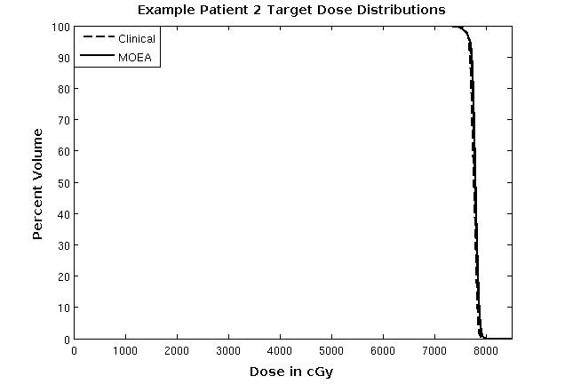
(b)

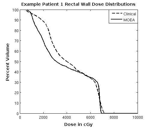
(c)

(d)

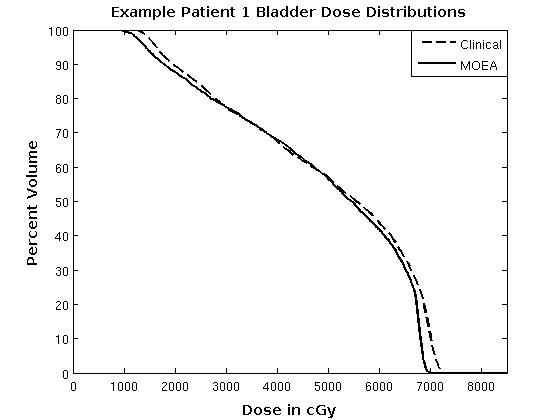
(e)

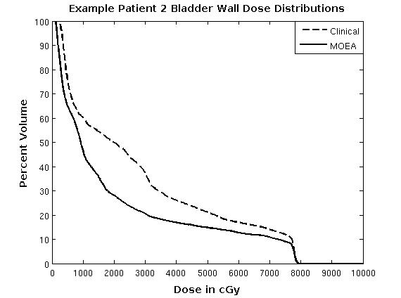
(f)

Figure 5: DVH comparisons for bladder, bladder wall, rectal wall, and PTV are made between plans selected from the population produced by the MOEA and plans produced using the current clinical inverse planning method.

The DVH comparisons for the target, rectal wall, and bladder for case 1 are shown in figures 5a-5c. The minimum target dose requirements were matched for these plans; however, the uniformity of the target dose distribtuion and lower maximum target dose were better for the MOEA plan. As this patient was more difficult especially with regards to the proximity of the entire bladder with the target, improvement of the MOEA OAR distributions over the clinical plan was modest. 32% of the volume of the rectum was inside the target, and some of this volume received higher dose in the MOEA plan. Once outside the PTV, the dose to the rectum dropped off more quickly for the MOEA than for the plan produced using the current clinical protocol.

The DVH comparisons for the target, rectal wall, and bladder wall for case 2 are shown in figures 5d-5f. For this prostate patient example, there was more separation between the OARs and the target, and this resulted in a greater potential for improvement using the MOEA. The target distributions nearly overlap, with the clinical plan’s coldest 1% of voxels below 75.5Gy versus 75.4Gy for the MOEA plan, and the clinical plan’s hottest 1% of voxels above 79.1 Gy versus 79.3 Gy for the MOEA plan. Dose levels for both the bladder and especially the rectum are much lower for the MOEA plan over the entire DVH.

3.6 Estimation of the Pareto front

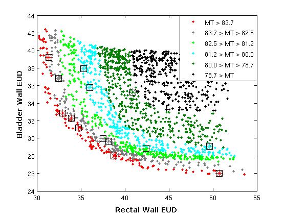
(b)

Figure 6: Plots for short multiobjective optimizations mapped onto an approximation of the Pareto front. Rectum and bladder EUD values are plotted with the target variance objective (MT) shown in color. The plans from the long optimization runs are represented as solid circles that make up most of the graphs. The plans resulting from the quick optimization are shown with asterisks using the same colorscale and surrounded by a black square for easier viewing.

The same two cases were used to investigate the ability of the MOEA to approximate the true Pareto front. For case 1, a long multiobjective optimization generated 9118 individuals in 12.6 hours without domination advantage in order to approximate the true Pareto front. Results were compared to 25 shorter optimizations that each generated 200 individuals using domination advantage. Figure 6a plots the results from one of the 25 short runs performed using domination advantage against the long optimization without using it. A similar comparison using case 2 was also performed using both a long (5000 individuals) run and 25 short runs (200 individuals) each. Results from one of the short runs is plotted with the long run results in Figure 6b.

For case 1, each individual in the long run dominated only $D_{C}$ = 0.20% $\pm$ 0.05% of the population generated using the short optimization. For case 2, each individual in the true Pareto front dominated an average of only $D_{C}$ = 0.14% $\pm$ 0.04% of the population generated using the short optimization. This demonstrates how quickly the algorithm with domination advantage approaches the Pareto front. The smaller populations were diverse and covered a wide range of the Pareto front, but certain regions characterized by diminishing returns were missed when using the domination advantage feature.

In order to see if the small performance improvement using domination advantage in short runs (Section 3.3) translated to longer runs, the long optimization runs described in the previous paragraph were repeated with and without domination advantage. For case 1, each individual in the long optimization using domination advantage dominated only $D_{C}$ = 0.009% of the population generated using the long optimization without domination advantage with $D_{C}$ = 0.004% in reverse. For case 2 each individual produced using domination advantage dominated only $D_{C}$ = 0.005% of the population generated using the long optimization without domination advantage, and the comparison was $D_{C}$ = 0.028% in reverse. Results suggest that for very long runs that closely approximate the Pareto front, domination advantage may slow convergence slightly, but differences are very small. Note that without the single fitness function domination advantage feature described in section 2.1.2, the MOEA would never get within $\sim\epsilon$ of the Pareto front using domination advantage, because all new individuals only slightly better than the existing population would have been eliminated.

4 Discussion

We have reported on the development of a hierarchical multiobjective optimization algorithm that couples a stochastic evolutionary algorithm with a fast deterministic one. The multiobjective nature of the algorithm reflects our view that IMRT planning requires exploring possible tradeoffs between competing clinical goals. The decision making strategy that must be coupled with the the multiobjective optimization has a profound influence on the structure of the algorithm. The current standard clinical decision making strategy supported by commercial inverse planning systems takes an interactive approach in which a plan is generated, evaluated by a human user, and a new search is made if necessary. Unfortunately, these systems do not provide any method for performing an efficient and effective search of all possible tradeoffs between objectives. While the result is usually better than achievable with 3D conformal techniques, the decision maker is not aware of the large number of other feasible solutions that may be better.

Another multiobjective method is the a posteriori approach in which a set of Pareto optimal plans are found first, and then this set is evaluated by a decision maker to select one. This is the nature of our MOEA and is a fairly popular approach for multiobjective problems in general [5, 18]. It has the advantage that the user does not have to determine relative importance amongst objectives before achievable tradeoffs are known. However, this comes at the price of time since there is little guidance in the search procedure. We have used several heuristic methods to focus the search. In addition, the domination advantage niche effect is designed to limit the final number of plans to the number that our decision process can handle. Bortfeld, Craft and colleagues have devised an alternative approach in which only convex objectives are used, the Pareto front is systematically mapped and calculation times are reduced by interpolating solutions[19, 20, 21, 22, 23]. Specially designed software allows the decision maker to steer between solutions on the Pareto front and observe the trade-offs of the different regions. Another systematic search approach was taken by Lahanas and colleagues [24, 25] in which attention was focused on the method of completely mapping the Pareto front with a simple decision making approach used a posteriori. An early paper by Yu which focused on brachytherapy and radiosurgical planning presented an excellent discussion of multiobjective optimization in radiation therapy [26]. He devised a plan ranking system that required some a priori importance input but used a simulated-annealing method to introduce some fuzziness and to broaden the search space. He also included a ”satisficing” condition that functioned similarly to our protocol objectives.

An a priori approach to multiobjective decision making in multiobjective optimization is the third alternative. Prior methods have the advantages of being among the fastest and providing a single solution. Jee et al [27] describe a method using the technique of lexigraphic ordering in which prior ranking of objectives leads to a sequence in which the first objective is satisfied and then turned into a constraint as the second objective is optimized and so on for the remainder. This is somewhat similar to our shifting the use of our protocol objectives between the second and third stages, but we make no preference between the objectives and all are satisfied simultaneously before transforming them to constraints.

Our use of an evolutionary algorithm was determined by its extensive use in multiobjective optimization in other fields [5] and because this type of algorithm can handle a much wider range of objective types than can deterministic algorithms. As with other aspects of our approach, the trade-off hinges on the speed of convergence. We used a hierarchical approach, coupled with the multiple stages, in order to mitigate this issue, and our results demonstrate that the performance is acceptable in a clinical setting. Wu and Zhu used a genetic algorithm for 3D conformal optimization to optimize the weighting factors [4]. Although they did not explicitly use Pareto optimality, their choice of a genetic algorithm was based on a recognition of the multiobjective nature of the problem and a desire to be flexible with respect to single objectives. Evolutionary algorithms have found their greatest use for the solution of explicitly non-convex objectives, such as the problem of number and orientation of the radiation beams [7, 25, 28, 29] and the integration of leaf sequencing and intensity optimization [30, 31] . Many other objectives in IMRT planning are also non-convex such as dose-volume objectives. For certain situations, it has been found that becoming trapped in local minima may be unlikely [32] or mathematical techniques are able to be applied to linearize non-convex objectives or approximate them with a convex surrogate [20, 33].

A critical component of any multiobjective optimization is the means by which two objects with multiple characteristics are compared or rated. A common example is the comparison of a dose-volume histogram from two different plans. When the DVHs do not cross, one can determine which is clearly better; when they do cross, ”better” depends on the decision variables. This is the essence of Pareto optimality. In our IMRT optimization, we removed plans that were dominated within some epsilon since those plans were clinically similar or worse in every aspect when compared to other plans. When comparing algorithms or optimization methods, a similar multiobjective approach can be taken. In our evaluation of different versions of our algorithm, we found it more useful to base our definition of ”better” on a statistical comparison using Pareto dominance as the defining criterion. A flexible multiobjective algorithm as described in this paper is the ideal means for making such comparisons which are more convincing than alternatives that are commonly used.

5 Conclusion

A multiobjective evolutionary algorithm was developed to find a diverse set of Pareto optimal and clinically acceptable IMRT plans. The novel selection method, flexible population size, and optimized mutation rates improved performance. The population diversity and size was effectively controlled using a niche effect, ”domination advantage”. The protocol objectives and multiple stages used in reproduction and selection guided the optimization to those regions of plan space that met clinical criteria. Key features of the algorithm are the ability to use any functional form of individual objectives and the ability to tailor the number and diversity of the output to the decision making environment.

6 Acknowledgements

Thanks to Stephanie Banerian for the computer and technical support. This work was supported by NIH 1-R01-CA112505.

Figure 2: Plot comparing the objectives of the final populations of plans resulting from the hierarchical approach with that of a standard genetic algorithm. The standard genetic algorithm is shown as asterisks, and the hierarchical approach is shown as solid circles. The color reflects the target maximum dose (MT), the target variance objective. Lower values in all objectives are more optimal.

Figure 3: Plot demonstrating the effect domination advantage has on a population of plans. The plans resulting from the hierarchical approach without using domination advantage are shown as asterisks, and those using domination advantage are shown as open squares. Maximum target dose (MT), the target variance objective, is displayed in color. Lower values in all objectives are more optimal.

(a)

(a)

References

- [1] J Meyer, M H Phillips, P S Cho, I Kalet, and J N Doctor. Application of influence diagrams to prostate intensity-modulated radiation therapy plan selection. Phys Med Biol, 49:1637–1653, 2004.
- [2] W P Smith, J Doctor, J Meyer, I J Kalet, and M H Phillips. A decision aid for IMRT plan selection in prostate cancer based on a prognostic Bayesian network and a Markov model. Artificial Intelligence in Medicine, 46:119–130, 2009.
- [3] G A Ezzell. Genetic and geometric optimization of three-dimensional radiation therapy treatment planning. Med Phys, 23:293–305, 1996.
- [4] X Wu and Y Zhu. An optimization method for importance factors and beam weights based on genetic algorithms for radiotherapy treatment planning. Phys Med Biol, 46:1085–99, 2001.
- [5] C A C Coello, D A Van Veldhuizen, and G B Lamont. Evolutionary Algorithms for Solving Multi-objective Problems. Kluwer Academic/Plenum Publishers, New York, 2002.
- [6] A Osyczka. Evolutionary Algorithms for Single and Multicriteria Design Optimization. Physica-Verlag, Heidelberg, Germany, 2002.
- [7] E Schreibmann, M Lahanas, L Xing, and D Baltas. Multiobjective evolutionary optimization of the number of beams, their orientations and weights for intensity modulated radiation therapy. Phys Med Biol, 49:747–770, 2004.
- [8] A Niemierko. Reporting and analyzing dose distributions: A concept of equivalent uniform dose. Med Phys, 24:103–110, 1997.
- [9] A Niemierko. A generalized concept of equivalent uniform dose (EUD). Med Phys, 26:1100, 1999.
- [10] G Luxton, P J Keall, and C R King. A new formula for normal tissue complication probability (NTCP) as a function of equivalent uniform dose (EUD). Phys Med Biol, 53, 2008.
- [11] S Breedveld, P R M Storchi, M Keijzer, and B J M Heijmen. Fast, multiple optimization of quadratic dose objective functions in imrt. Physics in Medicine and Biology, 51, 2006.
- [12] 1st International Conference: From Scientific Computing to Computational Engineering. BOXCQP: An algorithm for bound constrained convex quadratic problems, 2004.
- [13] M Phillips, M Kim, and A Ghate. Multiobjective optimization for IMRT using genetic algorithm. Med Phys, 35:2753, 2008.
- [14] I J Kalet, J P Jacky, M M Austin-Seymour, and J M Unger. Prism: A new approach to radiotherapy planning software. Int J Radiat Oncol Biol Phys, 36:451–461, 1996.
- [15] I J Kalet, J M Unger, J P Jacky, and M H Phillips. Prism system capabilities and user interface specification, version 1.2. Technical Report 97-12-02, Radiation Oncology Department, University of Washington, Seattle, Washington, 1997.
- [16] I J Kalet, J M Unger, J P Jacky, and M H Phillips. Experience programming radiotherapy applications in Common Lisp. In D D Leavitt and G Starkschall, editors, XII International Conference on the Use of Computers in Radiation Therapy, 1997.
- [17] M H Phillips, K M Singer, and A R Hounsell. A macropencil beam model: Clinical implementation for conformal and intensity modulated radiation therapy. Phys Med Biol, 44:1067–1088, 1999.
- [18] Y Collette and P Siarry. Multiobjective optimization: principles and case studies. Springer Verlag, New York, 2003.
- [19] D L Craft, T F Halabi, H A Shih, and T R Bortfeld. Approximating convex pareto surfaces in multiobjective radiotherapy planning. Medical Physics, 33, 2006.
- [20] D Craft, T Halabi, H A Shih, and T Bortfeld. An approach for practical multiobjective imrt treatment planning. Int J Radiat Oncol Biol Phys, 69, 2007.
- [21] T S Hong, D L Craft, F Carlsson, and T R Bortfeld. Multicriteria optimization in intensity-modulated radiation therapy treatment planning for locally advanced cancer of the pancreatic head. Int J Radiat Oncol Biol Phys, 72:1208–1214, 2008.
- [22] M. Monz, KH Küfer, TR Bortfeld, and C. Thieke. Pareto navigation. Physics in medicine and biology, 53:985–998, 2008.
- [23] C Thieke, K H Küfer, M Monz, A Scherrer, F Alonso, U Oelfke, P E Huber, J Debus, and T Bortfeld. A new concept for interactive radiotherapy planning with multicriteria optimization: first clinical evaluation. Radiother Oncol, 85:292–298, 2007.
- [24] M Lahanas, E Schreibmann, and D Baltas. Multiobjective inverse planning for intensity modulated radiotherapy with constraint-free gradient-based optimization algorithms. Phys Med Biol, 48:2843–2871, 2003.
- [25] M Lahanas, E Schreibmann, and D Baltas. Intensity modulated beam radiation therapy dose optimization with multiobjective evolutionary algorithms. In C M Fonseca, editor, Proc. 2nd Int. Conf. Evolutionary Multi-Criterion Optimization, EMO 2003 (Faro, Portugal, 8 11 April 2003), pages 439–47, 2003.
- [26] Y Yu. Multiobjective decision theory for computational optimization in radiation therapy. Med Phys, 24(9):1445–54, 1997.
- [27] K W Jee, D L McShan, and B Fraass. Lexicographic ordering: intuitive multicriteria optimization for imrt. Physics in Medicine and Biology, 52, 2007.
- [28] Q Hou, J Wang, Y Chen, and J M Galvin. Beam orientation optimization for IMRT by a hybrid method of the genetic algorithm and the simulated dynamics. Med Phys, 30:2360–7, 2003.
- [29] Y Li, J Yao, and D Yao. Automatic beam angle selection in imrt planning using genetic algorithm. Phys Med Biol, 49:1915–1932, 2008.
- [30] Y Li, J Yao, and D Yao. Genetic algorithm based deliverable segments optimization for static intensity-modulated radiotherapy. Phys Med Biol, 48:3353–3374, 2003.
- [31] C Cotrutz and L Xing. Segment based dose optimization using a genetic algorithm. Phys Med Biol, 48:2987–2998, 2003.
- [32] J Llacer, J O Deasy, T R Bortfeld, T D Solberg, and C Promberger. Absence of multiple local minima effects in intensity modulated optimization with dose-volume constraints. Phys Med Biol, 48:183–210, 2003.
- [33] H Romeijn, R Ahuja, J Dempsey, A Kumar, and J Li. A novel linear programming approach to fluence map optimization for intensity modulated radiation therapy treatment planning. Phys Med Biol, 48:3521–3542, 2003.