A Comparative Review of Dimension Reduction Methods in Approximate Bayesian Computation

Abstract

Approximate Bayesian computation (ABC) methods make use of comparisons between simulated and observed summary statistics to overcome the problem of computationally intractable likelihood functions. As the practical implementation of ABC requires computations based on vectors of summary statistics, rather than full data sets, a central question is how to derive low-dimensional summary statistics from the observed data with minimal loss of information. In this article we provide a comprehensive review and comparison of the performance of the principal methods of dimension reduction proposed in the ABC literature. The methods are split into three nonmutually exclusive classes consisting of best subset selection methods, projection techniques and regularization. In addition, we introduce two new methods of dimension reduction. The first is a best subset selection method based on Akaike and Bayesian information criteria, and the second uses ridge regression as a regularization procedure. We illustrate the performance of these dimension reduction techniques through the analysis of three challenging models and data sets.

=370pt Table 1: Relative $\overline{\mbox{RSSE}}$ for examples 1 and 2. The leftmost column shows the minimal $\overline{\mbox{RSSE}}$ when considering only one summary statistic (with no regression adjustment). Rightmost columns show relative $\overline{\mbox{RSSE}}$ using all summary statistics under no, homoscedastic and heteroscedastic regression adjustment. All $\overline{\mbox{RSSE}}$ are relative to the $\overline{\mbox{RSSE}}$ obtained when using no regression adjustment with all summary statistics. The score of the best method in each analysis (row) is emphasised in boldface One optimal statistic (no adj.) All summary statistics   No adj. Homo adj. Hetero adj. Example 1 $\tilde{\theta}$ $\mbox{$\bolds{-7}$}\$ 0 $-3$ $-3$ $\rho$ $9\ \mbox{($s_{5}$)}$ 0 $\mbox{$\bolds{-5}$}$ $-4$ $(\tilde{\theta},\rho)$ $7\ \mbox{($s_{1}$)}$ 0 $0$ $\mbox{$\bolds{-7}$}$ Example 2 $\alpha$ $6$ 0 $\mbox{$\bolds{-3}$}$ $\mbox{$\bolds{-3}$}$ $c$ $\mbox{$\bolds{-7}$}$ 0 $-5$ $-5$ $\rho$ $\mbox{$\bolds{-9}$}$ 0 $-8$ $-8$ $\mu$ $\mbox{$\bolds{-14}$}$ 0 $-5$ $-6$ $(\alpha,c,\rho,\mu)$ $5$ 0 $\mbox{$\bolds{-4}$}$ $\mbox{$\bolds{-4}$}$ ¯RSSEthanwhenincludingall6summarystatisticsevenwhenperformingregressionadjustment.Forallotherparametercombinations,usingasinglestatisticproducessubstantiallyworsethantherejectionalgorithmwithallsummarystatistics.Forallinferences[i.e.,of~θ,ρand(~θ,ρ)jointly],regressionadjustmentsgenerallyimprovetheinferencewhenusingallsixsummarystatistics,whichisconsistentwithpreviousresults(NunesBalding10).Theonlyexceptioniswhenjointlyestimating(~θ,ρ),wherehomoscedasticlinearadjustmentneitherdecreasesnorincreasestheerrorobtainedwiththepurerejectionalgorithm.

2andFigure1showtherelative¯RSSEobtainedundereachdimensionreductionmethodforeachparametercombinationandunderheteroscedasticregressionadjustment.Forallthreeexamples,morecompletetablesthatcontaintheresultsobtainedwithnoregressionadjustmentandhomoscedasticadjustmentcanbefoundinthesupplementaryinformationtothisarticle(Bluetal).

Table 2: Relative¯RSSEforexamples1--3fordifferentparametercombinationsusingeachmethodofdimensionreduction,andunderheteroscedasticregressionadjustment.Columnsdenotenodimensionreduction(All),BIC,AIC,AICc,theε-sufficiencycriterion(ε-suff),thetwo-stageentropyprocedure(Ent),partialleastsquares(PLS),neuralnetworks(NNet),minimumexpectedposteriorloss(Loss)andridgeregression(Ridge).All¯RSSEarerelativetothe¯RSSEobtainedwhenusingnoregressionadjustmentwithallsummarystatistics.Thescoreofthebestmethodineachanalysis(row)isemphasizedinboldface

		Best subset selection					Projection techniques			Regularization
	All	BIC	AIC	AICc	$\bolds{\varepsilon}$-suff	Ent	PLS	NNet$\bolds{\tabnoteref{1}}$	Loss	Ridge$\bolds{\tabnoteref{1}}$
$\tilde{\theta}$	$-3$	$-5$	$-5$	$-5$	$-6$	$\bolds{-11}$	$-6$	$-4$	$-7$	$1$
$\rho$	$-4$	$-6$	$-6$	$-6$	$0$	$\bolds{-12}$	$-7$	$-8$	$-7$	$-3$
$(\tilde{\theta},\rho)$	$-7$	$-7$	$-7$	$-7$	–	$\bolds{-24}$	$-16$	$-7$	$-6$	$-6$
$\alpha$	$-3$	$-15$	$-15$	$-15$	$0$	$\bolds{-17}$	$-13$	$-15$	$\bolds{-17}$	$-15$
$c$	$-5$	$\bolds{-15}$	$\bolds{-15}$	$\bolds{-15}$	$-8$	$\bolds{-15}$	$-8$	$-12$	$-9$	$-9$
$\rho$	$-8$	$\bolds{-16}$	$\bolds{-16}$	$\bolds{-16}$	$-8$	$\bolds{-16}$	$1$	$-12$	$-9$	$-10$
$\mu$	$-6$	$\bolds{-18}$	$\bolds{-18}$	$\bolds{-18}$	$-8$	$-13$	$-10$	$-13$	$-12$	$-12$
$(\alpha,c,\rho,\mu)$	$-4$	$\bolds{-19}$	$\bolds{-19}$	$\bolds{-19}$	–	$-13$	$-10$	$-9$	$-12$	$-11$
$\tau$	$-49$	$-47$	$-47$	$-48$	$-19$	$-52$	$-22$	$-20\mbox{$/$}{-}42$	$\bolds{-75}$	$-48\mbox{$/$}{-}48$
$\sigma$	$-45$	$-46$	$-47$	$-46$	$-15$	$-50$	$-15$	$-21\mbox{$/$}{-}37$	$\bolds{-56}$	$-43\mbox{$/$}{-}43$
$\xi$	$-27$	$-29$	$-29$	$-28$	$-13$	$-32$	$-28$	$-7\mbox{$/$}{-}41$	$-41$	$-26$$/$$\bolds{-44}$
($\tau,\sigma,\xi$)	$-39$	$-39$	$-40$	$-39$	–	$-42$	$-11$	$-4\mbox{$/$}{-}38$	$\bolds{-60}$	$-39\mbox{$/$}{-}32$

[

1]1

Fo

rt

he

thi

rd

ex

a

m

ple

,th

ef

irs

tv

al

ue

is

fo

un

db

yi

nt

eg

ra

tin

go

utt

he

re

gu

lar

iz

ati

on

pa

ra

me

ter

,w

h

er

ea

st

he

se

co

nd

on

eis

fo

un

db

yc

ho

osi

ng

an

opt

im

alr

eg

ul

ari

za

tio

np

ar

a

me

ter

wi

th

cr

os

s-v

ali

da

tio

n.

In

ex

a

m

ple

s1

an

d2,

int

eg

ra

tio

no

ve

rt

he

re

gu

lar

iz

ati

on

pa

ra

me

ter

isp

er

fo

r

me

d.

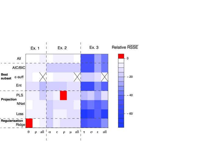
Figure 1: Relative¯RSSEforthedifferentmethodsofdimensionreductioninthethreeexamples.All¯RSSEarerelativetothe¯RSSEobtainedwhenusingnoregressionadjustmentwithallsummarystatistics.Methodsofdimensionreductionincludenodimensionreduction(All),AIC/BIC,theε-sufficiencycriterion(ε-suff),thetwo-stageentropyprocedure(Ent),partialleastsquares(PLS),neuralnetworks(NNet),minimumexpectedposteriorloss(Loss)andridgeregression(Ridge).Thecrossescorrespondtosituationsforwhichthereisnoresultavailable.

4.2 Example 2: The Fitness Cost of Drug Resistant Tuberculosis

We now consider an example of Markov processes for epidemiological modeling. If a pathogen, such as Mycobacterium tuberculosis, mutates to gain an evolutionary advantage, such as antibiotic resistance, it is biologically plausible that this mutation will come at a cost to the pathogen’s relative fitness. Based on a stochastic model to describe the transmission and evolutionary dynamics of Mycobacterium tuberculosis, and based on incidence and genotypic data of the IS6110 marker, LucianiEtAl09 estimated the posterior distribution of the pathogen’s transmission cost and relative fitness. The model contained $q=4$ free parameters: the transmission rate, $\alpha$, the transmission cost of drug resistant strains, $c$, the rate of evolution of resistance, $\rho$, and the mutation rate of the IS6110 marker, $\mu$.

LucianiEtAl09 summarized information generated from the stochastic model through $p=11$ summary statistics. These statistics were expertly elicited as quantities that were expected to be informative for one or more model parameters, and included the number of distinct genotypes in the sample, gene diversity for sensitive and resistant cases, the proportion of resistant cases and measures of the degree of clustering of genotypes, etc. It is considered likely that there is dependence and potentially replicate information within these statistics.

As before, we examine the relative performance of the statistics without using dimension reduction techniques. Table A Comparative Review of Dimension Reduction Methods in Approximate Bayesian Computation shows that for the univariate analysis of $c$, $\rho$ or $\mu$, performing rejection sampling ABC with a single, well-chosen summary statistic can provide an improved performance over a similar analysis using all 11 summary statistics, under any form of regression adjustment. In particular, the proportion of isolates that are drug resistant is the individual statistic which is most informative to estimate $c$ (with a relative $\overline{\mbox{RSSE}}$ of $-$7%) and $\rho$ ($-$9%). For the marker mutation rate, $\mu$, the most informative statistic is the number of distinct genotypes, with a relative $\overline{\mbox{RSSE}}$ of $-$14%. Conversely, an analysis using all summary statistics with a regression adjustment offers the best inferential performance for $\alpha$ alone, or for $(\alpha,c,\rho,\mu)$. These results provide support for recent arguments in favor of “marginal regression adjustments” (nott+fms11), whereby the univariate marginal distributions of a full multivariate ABC analysis are replaced by separately estimated marginal distributions using only statistics relevant for each parameter. Here, more precisely estimated margins can improve the accuracy of the multivariate posterior sample, beyond the initial analysis.

The performance results of each dimension reduction method are shown in Table 2 and Figure 1. In contrast with the previous example, here the use of the AIC/BIC criteria can substantially decrease posterior errors. For example, compared to the linear adjustment of all 11 parameters, which produces a mean relative $\overline{\mbox{RSSE}}$ between $-$3% and $-$8% depending on the parameter (Table 2), using the AIC/BIC criteria results in a relative $\overline{\mbox{RSSE}}$ of between $-$15% and $-$19%. The $\varepsilon$-sufficiency criterion produces more equivocal results, however, as the error is sometimes increased with respect to baseline performance (e.g., $+6\%$ when estimating $\alpha$ with homoscedastic adjustment) and sometimes reduced (e.g., $-$8% for $c$, $\rho$ and $\theta$ with heteroscedastic adjustment). As with the previous example, the entropy criterion provides a clear improvement to the ABC posterior, and this improvement is almost comparable to that produced by AIC/BIC. Finally, the projection and regularization methods mostly all provide comparable and substantive improvements compared to the baseline error, with only partial least squares producing more equivocal results (e.g., $+1\%$ when estimating $\rho$).

Based on these results, the loose performance ranking of the dimension reduction methods determines the worst performers to be the standard least squares regression adjustment (with a mean relative $\overline{\mbox{RSSE}}$ of $-$5%), the $\varepsilon$-sufficiency approach ($-$6%) and partial least squares ($-$8%). These are followed by ridge regression ($-$11%), neural networks and the posterior loss method ($-$12%). The best performing methods for this analysis are the two-stage entropy-based procedure ($-$15%) and the AIC/BIC criteria ($-$17%).

In this example, it is interesting to compare the performance of the standard linear regression adjustment of all 11 summary statistics (mean relative $\overline{\mbox{RSSE}}$ of $-$5%) with that of the ridge regression equivalent (mean relative $\overline{\mbox{RSSE}}$ of $-$11%). The increase in performance with ridge regression may be attributed to its more robust handling of multicolinearity of the summary statistics than under the standard regression adjustment. To see this, Figure 2 illustrates the relationship between the relative $\overline{\mbox{RSSE}}$ (again, relative to using all summary statistics and no regression adjustment) and the condition number of the matrix $X^{\top}WX$, for both the standard regression (top panel) and ridge regression (bottom panel) adjustments based on inference for $(\alpha,c,\rho,\mu)$. The condition number of $X^{\top}WX$ is given by $\kappa=\sqrt{\lambda_{\mathrm{max}}/\lambda_{\mathrm{min}}}$, where $\lambda_{\mathrm{max}}$ and $\lambda_{\mathrm{min}}$ are the largest and smallest eigenvalues of $X^{\top}WX$. Extremely large condition numbers are evidence for multicolinearity.

Figure 2: Scatterplots of relative RSSE versus the condition number of the matrix $X^{\top}WX$ for linear least squares (top) and ridge (bottom) regression adjustments. Points are based on joint inference for $(\alpha,c,\rho,\mu)$ in example 2 using 1000 randomly selected vectors of summary statistics, $s^{i}$, as “observed” data. When the minimum eigenvalue, $\lambda_{\mathrm{min}}$, is zero, the (infinite) condition number is arbitrarily set to be $10^{25}$ for visual clarity (open circles on the scatterplot).

Figure 2 demonstrates that for large values of the condition number (e.g., for $\kappa>10^{8}$), the least-squares-based regression adjustment clearly performs very poorly. The region of $\kappa>10^{8}$ corresponds to almost 5% of all simulations, and for these cases the relative error is hugely increased (w.r.t. rejection) to anywhere between 5% and 200%. In contrast, for ridge regression, the relative errors corresponding to $\kappa>10^{8}$ are not larger than the errors obtained for nonextreme condition numbers. This analysis clearly illustrates that, unlike ridge regression, the standard least squares regression adjustment can perform particularly poorly when there is multicolinearity between the summary statistics.

In terms of the original analysis of LucianiEtAl09 which used all eleven summary statistics with no regression adjustment (although with a very low value for $\epsilon$), the above results indicate that a more efficient analysis may have been achieved by using a suitable dimension reduction technique.

4.3 Example 3: Quality Control in the Production of Clean Steels

Our final example concerns the statistical modeling of extreme values. In the production of clean steels, the occurrence of microscopic imperfections (termed inclusions) is unavoidable. The strength of a clean steel block is largely dependent on the size of the largest inclusion. BortotEtAl07 considered an extreme value twist on the standard stereological problem (e.g., baddeley+j04), whereby inference is required on the size and number of 3-dimensional inclusions, based on data obtained from those inclusions that intersect with a 2-dimensional slice. The model assumes a Poisson point process of inclusion locations with rate parameter $\tau>0$ and that the distribution of inclusion size exceedances above a measurement threshold of $5\mu$m are drawn from a generalized Pareto distribution with scale and shape parameters $\sigma>0$ and $\xi$, following standard extreme value theory arguments (e.g., coles01).

The observed data consist of 112 cross-sectional inclusion diameters measured above $5\mu$m. The summary statistics thereby comprise 112 equally spaced quantiles of the cross-sectional diameters, in addition to the number of inclusions observed, yielding $p=113$ summary statistics in total. The ordering of the summary statistics creates strong dependences between them, a fact which can be exploited by dimension reduction techniques. BortotEtAl07 considered two models based on spherical or ellipsoidal shaped inclusions. Our analysis here focuses on the ellipsoidal model.

By construction, the large number ($2^{113}$) of possible combinations of summary statistics means that the best subset selection methods are strictly not practicable for this analysis, unless the number of summary statistics is reduced further a priori. In order to facilitate at least some comparison with the other dimension reduction approaches, for the best subset selection methods only, we consider six candidate subsets. Each subset consists of the number of observed inclusions in addition to 5, 10, 20, 50, 75 or 112 empirical quantiles of the inclusion size exceedances (the latter corresponds to the complete set of summary statistics). Due to the extreme value nature of this analysis, the parameter estimates are likely to be more sensitive to the precise values of the larger quantiles. As such, rather than using equally spaced quantiles, we use a scheme which favors quantiles closer to the maximum inclusion and we always include the maximum inclusion.

Table 3: Summary of the main features of the different methods of dimension reduction for ABC

Class	Method	Hyper-parameter	Choice of hyper-parameter	Computational burden
Best subset selection	AIC/BIC	None	–	Substantial/greedy alg.
	$\varepsilon$-suff	$T(\theta)$	User choice	Substantial/greedy alg.
	Ent	None	–	Substantial/greedy alg.
Projection techniques	PLS	Number of PLS components, $k$	Cross-validation	Weak
	NNet	Regularization parameter, $\lambda$	Integration or cross-validation	Moderate (optimization algorithm)
	Loss	Choice of basis functions	BIC	Weak (closed-form solution)
Regularization	Ridge	Regularization parameter, $\lambda$	Integration or cross-validation	Weak (closed-form solution)

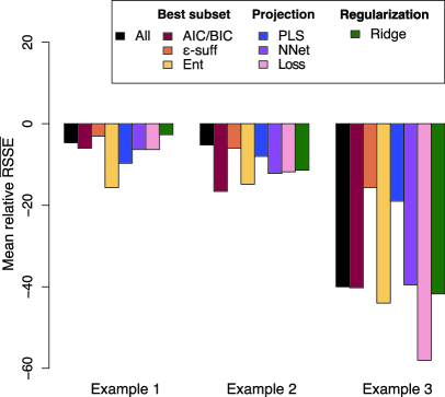
Figure 3: Mean relative $\overline{\mbox{RSSE}}$ values using each method of dimension reduction and for each example. Methods of dimension reduction include no dimension reduction (All), AIC/BIC, the $\varepsilon$-sufficiency criterion ($\varepsilon$-suff), the two-stage entropy procedure (Ent), partial least squares (PLS), neural networks (NNet), minimum expected posterior loss (Loss) and ridge regression (Ridge). For examples 1 and 2, the results for ridge regression and neural networks estimate $m(s)$ and $\sigma^{2}(s)$ have been obtained by taking the pointwise median curve over varying values of the regularization parameter; $\lambda=10^{-3},10^{-2}$ and $10^{-1}$ (see introduction to Section LABEL:sectionexamples). For example 3, an optimal value of $\lambda$ was chosen based on a cross-validation procedure (see Section 4.3).

The relative $\overline{\mbox{RSSE}}$ obtained under each dimension reduction method is shown in Table 2 and Figure 1. In comparison to an analysis using all 113 summary statistics and regression adjustment (the “All” column), the best subset selection approaches do not in general offer any improvement. While the entropy-based method provides a slight improvement, the relative $\overline{\mbox{RSSE}}$ under the $\varepsilon$-sufficiency criterion is substantially worse (along with partial least squares). Of course, these results are limited to the few subsets of statistics considered and it is possible that alternative subsets could perform substantially better. However, it is computationally untenable to evaluate this possibility based on exhaustive enumeration of all subsets.

When using neural networks to perform the regression adjustment based on computing the pointwise median of the $m(s)$ and $\sigma^{2}(s)$ estimates, obtained using varying regularization parameter values (see the introduction to Section LABEL:sectionexamples), the relative performance is quite poor (left-hand side $\overline{\mbox{RSSE}}$ values in Table 2). The mean relative $\overline{\mbox{RSSE}}$ is $-$13% for neural networks, compared to $-$40% for heteroscedastic least squares regression. As an alternative approach, rather than averaging over the regularization parameter $\lambda$, we rather choose the value of $\lambda\in\{10^{-3},10^{-2},10^{-1}\}$ that minimizes the leave-one-out error of $\theta$ [equation (LABEL:eqnPLSLOO)]. This approach considerably improves the performance of the network (right-hand side $\overline{\mbox{RSSE}}$ values in Table 2) with the mean relative $\overline{\mbox{RSSE}}$ improving to the same level as for heteroscedastic regression. Adopting the same procedure to determine the regularization parameter within ridge regression, there is also a mean gain in performance from $-$39% to $-$42%, although the joint parameter inference on $(\tau,\sigma,\xi)$ actually performs worse under this alternative approach. The variability in these results highlights the importance of making an optimal choice of the regularization parameter for an ABC analysis.

The minimum expected posterior loss approach performs particularly well here. This approach has also been shown to perform well in a similar analysis: that of performing inference using quantiles of a large number of independent draws from the (intractable) $g$-and-$k$ distribution (fernhead+p11).

The loose performance ranking of each of the dimension reduction methods finds that the worst performers are the $\varepsilon$-sufficiency criterion (with a mean relative $\overline{\mbox{RSSE}}$ of $-$16%) and partial least squares ($-$19%). Neural networks and AIC/BIC perform just as well as standard least squares regression ($-$40%), ridge regression slightly outperforms standard regression ($-$42%) and the entropy-based approach is a further slight improvement at $-$44%. The clear winner in this example is the posterior loss approach with a mean relative $\overline{\mbox{RSSE}}$ of $-$58%.

5 Discussion

The process of dimension reduction is a critical and influential part of any ABC analysis. In this article we have provided a comparative review of the major dimension reduction approaches (and introduced two new ones) in order to provide some guidance to the practitioner in choosing the most appropriate technique for their own analysis. A summary of the qualitative features of each dimension reduction method is shown in Table 3, and a comparison of the relative performances of each method for each example is illustrated in Figure 3. As with each individual example, we may compute an overall performance ranking of the dimension reduction methods by averaging the mean relative $\overline{\mbox{RSSE}}$ values over the examples. Performing worse, on average, than a standard least squares regression adjustment with no dimension reduction (with an overall mean relative $\overline{\mbox{RSSE}}$ of $-$17%) is the $\varepsilon$-sufficiency technique ($-$8%) and partial least squares ($-$12%). Performing better, on average, than standard least squares regression is ridge regression and neural networks ($-$19%) and AIC/BIC ($-$21%). In this study, the top performers, on average, were the entropy-based procedure and the minimum expected posterior loss approach, with an overall mean relative $\overline{\mbox{RSSE}}$ of $-$25%. It is worth emphasizing that the potential gains in performing a regression adjustment alone (with all summary statistics and no dimension reduction) can be quite substantial. This suggests that regression adjustment should be an integral part of the majority of ABC analyses. Further gains in performance can then be obtained by combining regression adjustment with dimension reduction procedures, although in some cases (such as with the $\varepsilon$-sufficiency technique and partial least squares) performance can sometimes worsen.

While being ranked in the top three, a clear disadvantage of the entropy-based procedure and the AIC/BIC criteria is the quantity of computation required. This primarily occurs as the best subset selection procedures require evaluation of all $2^{p}$ potential models. For examples 1 and 2, a greedy algorithm was able to find the optimum solution in a reasonable time. This was not possible for example 3. Additionally, in this latter case, for the subsets of summary statistics considered, the performance obtained by implementing computationally expensive methods of dimension reduction was barely an improvement over the computationally cheap, least squares regression adjustment. This raises the important point that the benefits of performing potentially expensive forms of dimension reduction over, say, the simple linear regression adjustment, should be evaluated prior to their full implementation. We also note that the second stage of the entropy-based method (Section LABEL:secentropy) targets minimization of (LABEL:eqnmrsse), the same error measure used in our comparative analysis. As such, this approach is likely to be numerically favored in our results.

The top ranked (ex aequo) minimum expected posterior loss approach particularly outperformsother dimension reduction methods in the final example (the production of clean steels). In such analyses, with large numbers of summary statistics (here $p=113$), nonlinear methods such as neural networks may become overparametrized, and simpler alternatives, such as least squares or ridge regression adjustment, can work more effectively. This is naturally explained through the usual bias-variance trade-off: more complex regression models such as neural networks reduce the bias of the estimate of $m(s)$ [and optionally $\sigma^{2}(s)$], but in doing so the variance of the estimate is increased. This effect can be especially acute for high-dimensional regression (geman1992neural).

Our analyses indicate that the original leastsquares, linear regression adjustment (Beaumont,Zhang and Balding (BeaumontEtAl02)) can sometimes perform quite well, despite its simplicity. However, the presence of multicolinearity between the summary statistics can cause severe performance degradation, compared to not performing the regression adjustment (see Figure 2). In such situations, regularization procedures, such as ridge regression (e.g., example 2 and Figure 2) and projection techniques, can be beneficial.

However, an important issue with regularization procedures, such as neural networks and ridge regression, is the handling of the regularization parameter, $\lambda$. The “averaging” procedure that was used in the first two examples proved quite suboptimal in the third, where a cross-validation procedure to select a single best parameter value produced much improved results. This problem can be particularly critical for neural networks with large numbers of summary statistics, $p$, as the number of network weights is much larger than $p$, and, accordingly, massive shrinkage of the weights (i.e., large values of $\lambda$) is required to avoid overfitting.

The posterior loss approach produced the superior performance in the third example. In general, a strong performance of this method can be primarily attributed to two factors. First, in the presence of large numbers of highly dependent summary statistics, the extra analysis stage in determining the most appropriate regression model (LABEL:fp11) by choosing $f(s)$ through, for example, BIC diagnostics, affords the opportunity to reduce the complexity of the regression in a simple and relatively low-parameterized manner. This was not a primary contributor in example 3, however, as the regression [equation (LABEL:fp11)] was directly performed on the full set of 113 statistics. Given the benefits of using regularization methods in this setting, it is possible that a ridge regression model would allow a more robust estimate of the posterior mean (as a summary statistic) as part of this process. Second, the posterior loss approach determines the number of summary statistics to be equal to the number of posterior quantities of interest—in this case, $q=3$ posterior parameter means. This small number of derived summary statistics naturally allows more precise posterior statements to be made, compared to dimension reduction methods that produce a much larger number of equally informative statistics. Of course, the dimension advantage here is strongly related to the number of parameters ($q=3$) and summary statistics ($p=113$) in this example. However, it is not fully clear how any current methods of dimension reduction for ABC would perform for substantially more challenging analyses with considerably higher numbers of parameters and summary statistics. This is because the curse of dimensionality in ABC (Blum10) has tended to restrict existing applications of ABC methods to problems of moderate parameter dimension, although this may change in the future.

What is very apparent from this study is that there is no single “best” method of dimension reduction for ABC. For example, while the posterior loss and entropy-based methods were the best performers for example 3, AIC and BIC were ranked first in the analysis of example 2, and partial least squares outperformed the posterior loss approach in example 1. A number of factors can affect the most suitable choice for any given analysis. As discussed above, these can include the number of initial summary statistics, the amount of dependence and multicolinearity within the statistics, the computational overheads of the dimension reduction method, the requirement to suitably determine hyperparameters and sensitivity to potentially large numbers of uninformative statistics.

One important point to understand is that all of the ABC analyses of this review were performed using the rejection algorithm optionally followed by some form of regression adjustment. While alternative, potentially more efficient and accurate methods of ABC posterior simulation exist, such as Markov chain Monte Carlo or sequential Monte Carlo based samplers, the computational cost of separately implementing such an algorithm $2^{p}$ times (in the case of best subset selection methods) means that such dimension reduction methods can become rapidly untenable, even for small $p$. The price of the benefit of using the more computationally practical, fixed large number of samples is that decisions on the dimension reduction of the summary statistics will be made on potentially worse estimates of the posterior than those available under superior sampling algorithms. As such, the final derived summary statistics may in fact not be those which are most appropriate for subsequent use in, for example, Markov chain Monte Carlo or sequential Monte Carlo based algorithms.

However, this price is arguably a necessity. It is practically important to evaluate the performance of any dimension reduction procedure in a given analysis. Here we used a criterion [the $\overline{\mbox{RSSE}}$ of equation (LABEL:eqnmrsse)] that is based on a leave-one-out procedure. When using a fixed, large number of samples, evaluation of such a performance diagnostic is entirely practicable, as no further model simulations are required. This idea is also relevant to methods of dimension reduction for model selection (barnesetal11; Marin12) where a misclassification rate based on a leave-one-out procedure can serve as a comparative criterion.

References

- Abdi and Williams (2010) {barticle}[author] \bauthor\bsnmAbdi, \bfnmH.\binitsH. and \bauthor\bsnmWilliams, \bfnmL. J.\binitsL. J. (