1 Introduction

The purpose of this study is to examine the functional dependence of sea ice brightness temperature on ice thickness at frequencies measured by the Advanced Microwave Scanning Radiometer on EOS (AMSR-E). That is, to generate a set of brightness temperature-thickness ($T_{b}$-$h$) curves. Several studies have demonstrated a relationship between ice thickness and SSM/I or AMSR-E brightness temperatures (Martin et al., 2004; Naoki et al., 2008; Kwok et al., 2007; Hwang et al., 2007) with at least one attempt to use this relationship for the purpose of ice thickness retrieval (Martin et al., 2004).

This relationship, however, is not a direct one in the sense that, all other things begin equal, changes in ice thickness will not necessarily affect microwave emissions at AMSR-E frequencies. Even at 6.8 GHz, the penetration depth is far smaller than all but the thinnest of ice sheets. The relationship is caused by the fact that thinner, newer ice, has different physical properties than those of older, thicker ice. In particular it tends to be more saline, especially in the top layers.

Three processes ensure that newer, thinner ice is, on average, more saline than older, thicker ice (Tucker et al., 1992; Eicken, 1992; Weeks and Ackley, 1985; Vancoppenolle et al., 2007; Ehn et al., 2007), especially in the top layers. As new ice is formed, most of the salt gets expelled, except for a small amount that is included as pockets of highly saline brine. The faster the ice grows, the more brine is included. Since thin ice conducts heat more quickly, it will grow faster than thicker ice on average. As a growing ice sheet cools, some of the water in the brine will freeze. Since ice is less dense than brine, increasing pressure in the brine pockets will cause some of the brine to be expelled from both the top and bottom of the ice sheet, producing the characteristic ’C’-shaped profile of first-year ice. Finally, as the ice ages, thawing will produce channels through which much of the brine can drain.

The causal relationship between salinity and brightness temperature is similarly circuitous, although it is a more definite one. Higher salinity produces a higher effective permittivity whose main effect, for optically thick ice, is to increase the polarization difference or second Stokes parameter. It is not just the salinity that affects the microwave signal. Changes in temperature will have a similar effect as well as a similar cause. That is, warmer ice will tend to have a higher effective permittivity and thinner ice will tend to be warmer, again because of heat conduction.

We use parameterised empirical relationships between ice thickness and salinity. Model profiles are fed to ice emissivity models to determine idealized relationships between brightness temperature and ice thickness.

2 Model set up

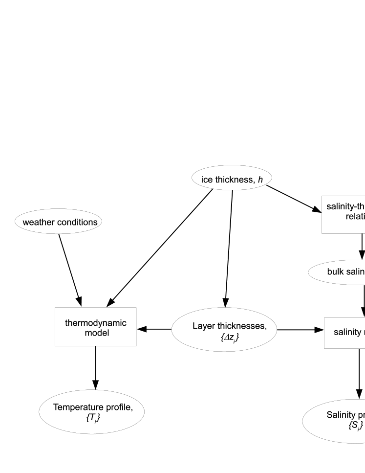
Figure 1: Data flow diagram describing the model set up, namely how the other parameters are derived from ice thickness. Rectangles are processes, ellipses are data. The salinity-thickness relation and the salinity model are described in Section 2.2. The thermodynamic model is described in Section 2.3

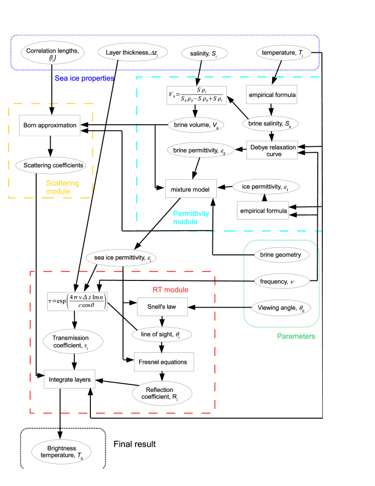
Figure 2: Detailed data flow diagram describing the complete ice emissivity model. Rectangles are processes, ellipses are data. The “mixture model” is described in Section 2.1. Other components are described elsewhere, see for instance Mills and Heygster (2011) and Wiesmann and Maetzler (1999a).

The boxes labelled, respectively, “Snell’s law”, “Fresnel equations”, “Integrate layers” and the box with the equation for the transmission coefficent correspond to equations (3), (1-2), (5-6) and (7-8) in Mills and Heygster (2011). The equations for fresh-water ice permittivity are contained in Hufford (1991). For other equations in the permittivity module, a good reference is Ulaby et al. (1986).

We use a layered, plane-parallel, radiative transfer (RT) model called Microwave Emissivity Model for Layered Snowpack (MEMLS) (Wiesmann and Maetzler, 1999a, b). The emissivity calculation can be divided into three main modules. First, effective relative permittivities must be calculated from the physical properties of each layer–chiefly, temperature and salinity. Second, scattering coefficients must also be calculated from values of correlation length. Finally, these permittivities and scattering coefficients are simultaneously integrated through the depth of the ice sheet. Before we can feed these quantities into the model, however, we must take account of the numerous and complex interrelationships between the different inputs, particularly since we are interested only in the functional dependence of brightness temperature on a single bulk property, i.e. ice thickness. For example, because of changes in relative brine volume at different temperatures and salinities, correlation lengths of the brine inclusions will be affected by these other two properties.

The emissivity model is described in the data flow diagram shown in Figure 2 including data inputs and parameters. The basic modules have a dashed outline. As can be seen, it is a quite a complex model comprising many separate yet interacting components. The model set up is shown in Figure 1.

Both ice thickness and the salinity profile (function of salinity with depth) will be affected by past weather conditions. In addition, the current temperature profile will be determined by both the ice thickness and prevailing weather conditions. For this reason, we have designed a simple thermodynamic model which can be used both to determine the temperature profile, and in a crude fashion, model ice growth. This model is described below, along with the other components.

The calculation of effective permittivities is described below. For scattering coefficients, we use the empirical model within MEMLS (Wiesmann and Maetzler, 1999b). We relate the correlation length to brine volume as follows:

$$l=l_{0}\sqrt{V_{b}}$$ (1)

where $l_{0}$ is a constant and $V_{b}$ is relative brine volume. For the case of randomly positioned, oriented cylinders, the correlation length in the transverse direction would be related to brine volume to the first power. For the case of randomly positioned spheres, it would be to the third power. (Maetzler, 1997) We take the second power, thus the brine inclusions are somewhere between a cylinder and a sphere.

The radiative transfer model will not be described in this report since it and similar models are covered in other publications — see for instance, Wiesmann and Maetzler (1999a) and Mills and Heygster (2011). We will note, however, that there is some descrepancy in the two models contained in the aforementioned publications as to when and how (by simply eliminating it or taking the absolute value) to drop the imaginary component of the reflection coefficients. In MEMLS, for instance, only the real part of the complex permittivity is used in the calculation of reflection coefficients. In Mills and Heygster (2011), by contrast, the imaginary part is carried right to the end of the calculation and real reflection coefficients produced by taking the absolute value. Using one method or the other can mean a difference of as much as 10 K. We have modified the MEMLS code so that calculations of reflection coefficients match the model described in Mills and Heygster (2011). When scattering is neglected in MEMLS, the two models agree to within half a Kelvin.

The viewing angle is set at 55 degrees, or the same as AMSR-E.

2.1 Model for effective permittivities

Figure 3: Comparison of the mixture model of Sihvola and Kong based on de-polarizability and the empirical mixture model of Vant using random values of temperature in the range of 251 to 271 K and salinity in the range of 0 to 15 psu.

Table 1: Correlation between Vant and Sihvola mixture models of effective permittivity for both real and imaginary components.

$\nu$	$r(\epsilon^{\prime})$	$r(\epsilon^{\prime\prime})$
0.1	0.994	0.929
0.2	0.994	0.928
0.4	0.995	0.942
0.8	0.995	0.974
1.0	0.996	0.981
2.0	0.995	0.984
4.0	0.995	0.983

Figure 4: Correlations with wavelength of regression coefficients between empirical and theoretical mixture models.

Figure 5: Validation of semi-emprical mixture model. All frequencies between 0.1 and 4 GHz.

Table 2: Fitted coefficients for semi-empirical mixture model.

The calculation of effective relative permittivity is one of the most important steps in the model. It is also the one of the least understood and most fraught with uncertainty. To calculate the effective permittivity, we use a semi-empirical model combining the empirical mixture model of Vant et al. (1978) and the theoretical one from Sihvola and au Kong (1988) based on the low-frequency limit. Vant et al. give an empirical mixture model based on fits of measured real and imaginary permittivity to brine volume:

$$\epsilon^{*}=aV_{b}+b$$ (2)

where $\epsilon^{*}$ is the effective permittivity (real or imaginary), $V_{b}$ is the relative brine volume and $a$ and $b$ are constants. Different constants have been acquired for frequencies between 0.1 and 4 GHz. To extend the frequency range of the Vant models, we combine it with the following theoretical, mixture model for oriented needles based on the low-frequency limit (Sihvola and au Kong, 1988):

$$\epsilon_{eff}=\epsilon_{1}+\frac{V_{b}(\epsilon_{2}-\epsilon_{1})\epsilon_{1}/\left[\epsilon_{1}+P(\epsilon_{2}-\epsilon_{1})\right]}{1-PV_{b}(\epsilon_{2}-\epsilon_{1})\left[\epsilon_{1}+P(\epsilon_{2}-\epsilon_{1})\right]}$$ (3)

where $\epsilon_{1}$ is the permittivity of the host material (ice), $\epsilon_{2}$ is the permittivity of the inclusion material (brine), and $P=0.5$ is the de-polarisation factor. It was observed that the results from (2) and (3) are closely correlated as shown in Figure 3, however they differ by both a constant factor (in the real part) and a coefficient (in both the real and imaginary parts). These parameters were found to vary closely with the wavelength, as shown in Figures 4.

Thus, the combined model is given as follows:

$$\epsilon_{semi}=(c_{1}/\nu+c_{2})\epsilon_{eff}^{\prime}+c_{3}/\nu+c_{4}+(c_{5}/\nu+c_{6})\epsilon_{eff}^{\prime\prime}i$$ (4)

where $\epsilon_{eff}=\epsilon_{eff}^{\prime}+\epsilon_{eff}^{\prime\prime}i$ is the effective permittivity from Equation (3), $\nu$ is frequency and $c_{1}$ through $c_{6}$ are fitted constants. Note that there is no constant term for the imaginary part, forcing the value to zero for zero brine volumes (pure ice is almost a perfect dielectric). We compare the derived semi-emprical model with the Vant model for a range of frequencies between 0.1 and 4. GHz, a range of salinities between 0 and 15 psu and a range temperatures between 251 and 271 K in Figure 5. The fitted coefficients, $c_{1}$ through $c_{6}$ are given in Table 2.1.

Finally, a note on brine volume. In Mills and Heygster (2011), brine volume was given as:

$$V_{b}=\frac{S}{S_{b}}$$ (5)

where $S_{b}$ is the brine salinity which, because of freezing point depression, can be calculated from temperature only. This is a rather crude approximation. A more accurate formula is as follows:

$$V_{b}=\frac{S\rho_{i}}{S_{b}\rho_{b}-S\rho_{b}+S\rho_{i}}$$ (6)

where $\rho_{i}$ and $\rho_{b}$ are the densities of ice and brine, respectively. This formula is found by writing the ratio of brine volume to ice volume in terms of density and salinity and solving. It directly connects the calculation of brine salinity (an accurate function of temperature only) with relative brine volume.

2.2 Salinity model

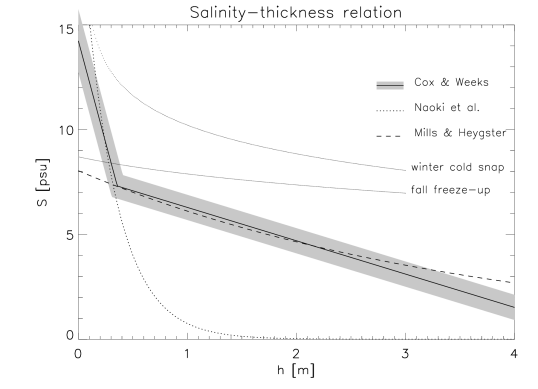
Figure 6: Different salinity-thickness relationships compared. Shading are residuals for the Cox and Weeks models.

Figure 7: Model salinity profiles for different bulk salinities in 0.5 psu increments, starting at 0.5psu and ending at 10psu. Ice depth is normalized.

Figure 6 shows plots of different salinity-thickness (S-$h$) curves which have been derived empirically and from a simple model (see below). Cox and Weeks (1974) provide the following piece-wise, linear fit of bulk salinity to ice thickness (solid curve):

$$S_{\mathrm{ave}}=\left\{\begin{array}[]{lr}14.24-19.39h;&h\leq 0.4m\\ 7.88-1.59h;&h>0.4m\end{array}\right.$$ (7)

where $S_{\mathrm{ave}}$ is bulk salinity and $h$ is ice thickness in metres. This is the only S-h curve that will be used in the study. Rather than trying the emissivity models with different curves, Cox and Weeks (1974) provide residuals for the curves. We will use these residuals, along with those supplied with the Vant effective permittivity models to compute an error bound for the final results (see below).

The other five curves are as follows. Naoki et al. (2008) generated an exponential fit (short-dashed curve) of surface salinity (top 10 cm) based on measurements conducted in the Sea of Okhotsk:

$$S=\exp(mh+k)$$ (8)

where $S$ is the salinity, $h$ is ice thickness and $m$ and $k$ are constants. Heygster et al. (2009) generated an exponential fit of ice core samples taken from the Weddell Sea (Eicken, 1992). Coefficients for equation (8) are $m=-3.55$ and $k=3.06358$ for the Naoki model and $m=-0.275$ and $k=8.04$ for Heygster et al. (2009). Notice that the Naoki curve roughly matches the left section of the Cox and Weeks curve, while the Mills and Heygster curve roughly matches the right section.

The dotted curves show results from the thermodynamic ice growth model (described in the next section) for two weather scenarios: fall freeze-up and a winter cold snap. These provide a reasonable range for thin ice (below 30 cm), however they over-estimate salinity for thick ice.

Two trials will be performed: one in which the ice is represented as a single layer, and one with a parameterized salinity profile. For the parameterized salinity profile, we use the ’S’-shaped model from Eicken (1992), but with the caveat that at values for bulk salinity below 2psu, it reverts to a flat profile in accordance with Granskog et al. (2006). This is shown in Figure 7.

2.3 Thermodynamic model

Table 3: Thermodynamic model parameters for the two weather scenarios

	Scenario
Parameter	Fall freeze-up	Winter cold snap
Wind speed [m/s]	2.	10.
Air temperature [K]	270.	260.
Relative humidity	0.5	0.1
Cloud-cover	0.5	0.1
Insolation [W/m2]	50.	0.

As mentioned in the introduction, it is not just ice salinity that lowers the brightness temperature of thin ice, it is also the temperature: thin ice conducts heat faster. This increase in temperature will have two effects: direct (hotter objects are brighter) and indirect (higher temperatures produce higher complex permittivities.) Therefore, for the multi-layer models, we calculate the surface temperature using a thermodynamic model based on certain assumed prevailing weather conditions. Since we assume the ice is in thermal equilibrium—valid if the ice is not too thick and the weather is changing relativly slowly— the temperature profile is linear.

The following equation relates the ice surface temperature to net heat flux:

$$hQ^{*}=k(T_{w}-T_{s})$$ (9)

where $T_{w}$ is the water temperature which is assumed to be constant at freezing (approximately -1.9^∘ C at a water salinity of 35 psu), $T_{s}$ is surface temperature and $k$ is the thermal conductivity of the ice. The net heat flux comprises the following components, with functional dependencies supplied:

$$Q^{*}=Q_{E}[e(T_{s})]+Q_{H}(T_{s})+Q_{SW}(T_{s}^{4})+Q_{LW}$$ (10)

The terms on the RHS are, from left to right: latent heat, sensible heat, longwave and shortwave; $e(T)$ is the saturation vapour pressure. The first two terms are approximated with simple parameterisations while the longwave flux is based on the Stefan-Boltzmann law. The shortwave flux is calculated primarily from geometric considerations based on the position of the Earth relative to the Sun. The following inputs are required for the model: surface- wind speed, humidity, air temperature and density (or pressure), cloud cover and date and time or insolation. (Cox and Weeks, 1988; Drucker et al., 2003; Yu and Lindsay, 2003) Inputs can be supplied to give a picture of the general weather conditions. For instance, fall freeze-up might be characterized by relatively mild temperatures, low winds, high humidity, high cloud cover and moderate insolation. By contrast, a winter cold snap would be characterized by low temperature, high winds, low humidity, clear conditions and little to no insolation. See Table 3. Equations (9) and (10) are solved with a numerical root-finding algorithm, specifically bisection (Press et al., 1992).

The model can also be used as a crude ice growth model. The rate of ice growth is:

$$g=\frac{Q^{*}}{L\rho_{i}}$$ (11)

where $L$ is the latent heat of fusion for water. Empirical equations for determining the initial brine entrapment in sea ice have been derived by Cox and Weeks (1988) and Nakawo and Sinha (1981) and take the form:

$$S=S_{0}f(g)$$ (12)

where $S_{0}$ is the salinity of the parent water and $f$ is an empirical function of ice growth rate.

As a qualitative validation of the salinity-thickness relations described in 2.2, this model is quite effective. As seen in Figure 6, the model considerably overestimates the actual salinities, especially as the ice get thicker. This is because it does not take into account brine drainage and expulsion.

2.4 Error

Figure 8: Error residuals for the Vant effective permittivity models plotted against wavelength. Fitted curves are shown.

Both the salinity-thickness relation from Cox and Weeks (1974) and the mixture models from Vant et al. (1978) are supplied with statistical error bounds (root-mean-square errors (RMSE) or residuals). We use these to generate error tolerances for the final $T_{b}$-thickness curves. Residuals from the Vant models were found to have a similar close correlation with wavelength as the relationship between the two effective permittivity models: see Figure 8. This relationship was use to extrapolate the residuals to higher frequencies. A Monte Carlo or “bootstrapping” (Press et al., 1992) method is used. Intitial salinities are perturbed with Gaussian deviates with zero mean and standard deviation equal to the residuals. So are the generated complex permittivities. The number of trials was chosen based on convergence of error estimates.

3 Results

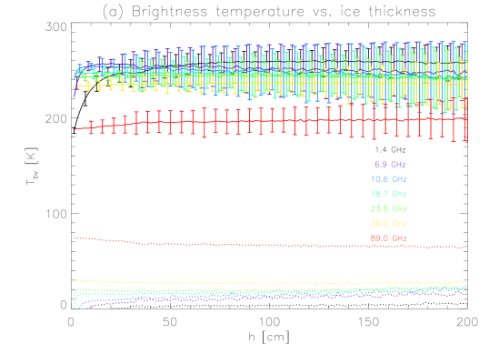
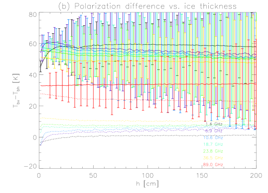
Figure 9: Modelled brightness temperature as a function of ice thickness using a single ice layer and constant temperature of 265K. Dotted lines show scattering component.

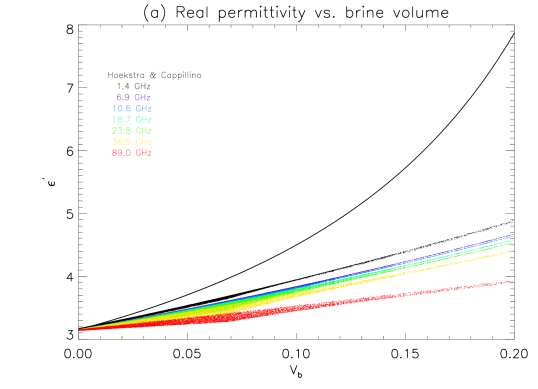
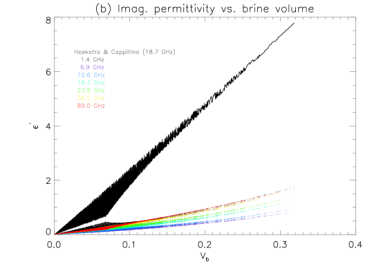
Figure 10: Comparison of modelled effective permittivities using Hoekstra and Cappillino (1971) and the semi-empirical model described in the text. The Hoekstra and Cappillino mixture model was used by Naoki et al. (2008) to model emissivity as a function of ice thickness.

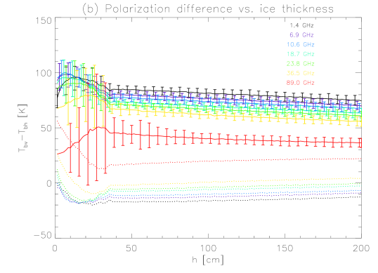
Figure 11: Modelled brightness temperature as a function of ice thickness using multiple (21) ice layers. Salinity profile has an ‘S’-shape while the temperature profiles is determined with a thermodynamic model. Both are described in the text. Dotted lines show scattering component.

Here the final $T_{b}$-thickness relations are presented. The error bounds are rigorous in the sense that those quantities with known error have been fully accounted for. However, there are many factors not accounted for in the model such as the possible effects of ice ridging and anisotropy of the brine inclusions. Factors without known error, such as the correlation length of the brine inclusions, have not been accounted for.

The dependence on ice thickness of vertically polarized brightness temperature for the single (ice) layer model is shown in Figure 9 along with error bars. Ice temperature was assumed to be 365 K. What these results show is a modest and fairly rapid increase in emissivity with thickness as the ice becomes progressively more opaque, thus less of the water shows through. Once the signal becomes “saturated” with only the ice emissions, the curve remains relatively flat, with an emissivity of close to one. The distance to saturation is controlled by the frequecy: from Equation (8) in Mills and Heygster (2011), the attenuation coefficient depends directly on the frequency. For all but the bottom two or three frequencies, the water layer hardly shows through even at the thinnest ice thickneses resulting in an almost constant emissivity.

These results contrast with the those of Naoki et al. (2008) in which both modelled and measured ice emissivity was shown to have a strong and slow increase with thickness. The reason for the difference lies in the modelled effective permittivies, which are shown in Figure 10. Naoki et al. use a mixture model that generates much larger values at higher salinities. It is this large real component that produces low emissities at thinner ice thicknesses. The changes in real permittivity will also produce higher polarisation differences at thinner ice thickness and this pattern can be seen weakly in Figure 9 (b). (See Heygster et al. (2009) and Mills and Heygster (2011) for an explanation.) It is this decrease in polarization difference that is frequently used to detect thin ice, as in Martin et al. (2005).

The $T_{b}$-thickness curves for the more sophisticated, multi-layer model are shown in Figure 11. 21 layers were used in the model. Note that this model shows a stronger increase/decrease in brightness-temperature/polarization difference with ice thickness, especially at higher frequencies. This is due mainly to the scattering component, which is shown by the dotted lines. Error bars for these curves are narrower because the random variations in effective permittivity in each layer will tend to cancel. Note that errors are higher for the polarization differences (in both models) because they were calculated from the root-sum-square of the errors in the horizontal and vertical.

4 Summary and conclusions

Radiative transfer-based emissivity models were run for all frequencies of the Advanced Microwave Scanning Radiometer on EOS (AMSR-E) instrument (6.925, 10.65, 18.7, 23.8, 36.5 and 89.0 GHz) as well as 1.4 GHz in order to determine the relationship of emissivity to sea ice thickness. Because of ice growth processes, ice salinity is normally inversely related to ice thickness. The satistical model of Cox and Weeks (1974) was used to relate bulk salinity to ice thickness. The emissivity model assumes plane parallel geometry; two versions were employed: one with only one ice layer (uniform properties throughout) and one with multiple layers. For the single layer model, a constant temperature of 265 K was used. For the multi-layer model, the salinity profile was modelled with the ‘S’-shaped profile from Eicken (1992), scaled to match the bulk salinity. For the temperature profile, a thermodynamic model was employed which assumed thermal equilibrium and weather conditions equivalent to fall freeze-up.

Complex effective permittivities to feed to the RT model were calculated from salinities and temperatures. Vant et al. (1978) derived measurement-based, statistical models that linearly relate effective permittivity to brine volume. These models were only generated for frequencies between 0.1 and 4 GHz. In order to extend the Vant models to higher frequencies, theoretical mixture models taken from Sihvola and au Kong (1988) and based on the low frequency limit were statistically adjusted to the Vant models.

Error tolerances were calculated using a Monte Carlo method based on the residuals supplied with both the Cox and Weeks salinity-thickness relation and with the Vant effective permittivity models.

When scattering is neglected, the brightness temperature is found to vary only slightly with ice thickness for both the single- and multi-layer models, except at the lower frequecies, where brightness temperature increases with ice thickness. The latter effect is caused by the greater translucency of the ice at lower frequencies: the water below shows through. The reason little change is observed at higher frequencies is because the effective permittivity models show only a weak increase in real permittivity with brine volume. Contrast this result to Naoki et al. (2008). Note that both the real and imaginary permittivities are almost linearly related to salinity.

Adding scattering produces much more variation with ice thickness of both brightness temperature and polarization difference, particularly in the multi-layer model. Below about 30 cm, the brightness temperature is seen to increase sharply with ice thickness, while above that it decreases gently, especially at the higher frequencies. This is in accordance with measurements where it is observed that thin ice has both a lower brightness temperature and higher polarization difference, while older, thicker ice tends to be radiometrically cooler. Meanwhile, the size of the scatterers ensure that scattering is greater at higher frequencies. It also makes sense that most of this difference is due to scattering: thinner ice is more saline, hence it will have both more and larger brine pockets. It also tends to be more granular, although this is not well accounted for in the models. For the multi-layer model, scattering in the horizontal polarization is larger than that in the vertical, a possibly questionable result.

One puzzling feature of the muliti-layer results is the low polarization difference for very thin ice (below 20 cm), especially at higher frequencies. This is due to the scattering component and does not accord well with measurements. To correct this, a better understanding of the relationship between scattering and ice physical properties is necessary.

Error bounds were larger for the single-layer model and reached as high as 50 K. For the multi-layer model, bounds high for thin ice thicknesses (again, as high as 50 K) but tended to be lower. Most were below 10 K, particularly for lower frequencies and higher ice thicknesses.

Better ice emissivity models require better estimates of ice effective permittivity, hence the design of a new, combined model. The correlation in wavelength of the Vant empirical models with the Sihvola and Kong theoretical models (based on the low-frequency limit) is likely significant, but a fuller understanding would require a deeper investment into the theory. A similar statement is true for the scattering components of the model in which the correlation length was related to brine volume using a simple, ad hoc assumption.

Understanding ice growth processes would be another area for future study since they are closely connected with ice emissivity. A simple ice growth model based on the thermodynamic model for ice temperature was used to qualitatively confirm the relationship of bulk salinity to thickness. Ice cores from the Weddell Sea were similarly modelled however the results are not shown here.

References

- Cox and Weeks (1988) Cox, G. and Weeks, W. (1988). Numerical simulations of the profile properties of undeformed first-year sea ice during the growth season. Journal of Geophysical Research, 93(C10):12499–12460.
- Cox and Weeks (1974) Cox, G. F. N. and Weeks, W. F. (1974). Salinity variations in sea ice. Journal of Glaciology, 13(67):109–120.
- Drucker et al. (2003) Drucker, R., Martin, S., and Moritz, R. (2003). Observations of ice thickness and frazil ice in the St. Lawrence Island polynya from satellite imagery, upward looking sonar, and salinity/temperature moorings. Journal of Geophysical Research, 108(C5).
- Ehn et al. (2007) Ehn, J. K., Hwang, B. J., Galley, R., and Barber, D. G. (2007). Investigations of newly formed sea ice in the Cape Bathurst polynya: 1. Structural, physical and optical properties. Journal of Geophysical Research, 112(C05002).
- Eicken (1992) Eicken, H. (1992). Salinity Profiles of Antarctic Sea ice: Field Data and Model Results. Journal of Geophysical Research, 97(C10):15545–15557.
- Granskog et al. (2006) Granskog, M., Kaartokallio, H., Kuosa, H., Thomas, D. N., and Vainio, J. (2006). Sea ice in the Baltic Sea–A review. Estuarine, Coastal and Shelf Science, 70:145–160.
- Heygster et al. (2009) Heygster, G., Hendricks, S., Kaleschke, L., Maass, N., Mills, P., Stammer, D., Tonboe, R. T., and Haas, C. (2009). L-Band Radiometry for Sea-Ice Applications. Technical Report final report for ESA/ESTEC Contract N. 21130/08/NL/EL, Institute of Environmental Physics, University of Bremen.
- Hoekstra and Cappillino (1971) Hoekstra, P. and Cappillino, P. (1971). Dielectric Properties of Sea and Sodium Chloride Ice at UHF and Microwave Frequencies. Journal of Geophysical Research, 76(20):4922–4931.
- Hufford (1991) Hufford, G. (1991). A model for the complex permittivity of ice at frequencies below 1 THz. International Journal of Infrared and Millimeter Waves, 12(7):677–682.
- Hwang et al. (2007) Hwang, B. J., Ehn, J. K., Barber, D. G., Galley, R., and Grenfell, T. C. (2007). Investigations of newly formed sea ice in the Cape Bathurst polynya: 2. Microwave emission. Journal of Geophysical Research, 112(C05003).
- Kwok et al. (2007) Kwok, R., Comiso, J., Martin, S., and Drucker, R. (2007). Ross Sea polynyas: Response of ice concentration retrievals to large areas of thin ice. Journal of Geophysical Research, 112(C12012).
- Maetzler (1997) Maetzler, C. (1997). Autocorrelation functions of granular media with free arrangement of spheres, spherical shells or ellipsoids. Journal of Applied Physics, 81(3).
- Martin et al. (2004) Martin, S., Drucker, R., Kwok, R., and Holt, B. (2004). Estimation of the thin ice thickness and heat flux for the Chukchi Sea Alaskan coast polynya from Special Sensor Microwave Imager data, 1990-2001. Journal of Geophysical Research, 109(C10012).
- Martin et al. (2005) Martin, S., Drucker, R., Kwok, R., and Holt, B. (2005). Improvements in the estimates of ice thickness and production in the Chukchi Sea polynyas derived from AMSR-E. Geophysical Research Letters, 32(L05505).
- Mills and Heygster (2011) Mills, P. and Heygster, G. (2011). Modelling sea ice emissivity at L-band and application to Pol-Ice campaign field data. IEEE Transactions on Geoscience and Remote Sensing, 49(2):612–627.
- Nakawo and Sinha (1981) Nakawo, M. and Sinha, N. K. (1981). Growth rate and salinity profile of first-year sea ice in the high arctic. Journal of Glaciology, 27(96):315–330.
- Naoki et al. (2008) Naoki, K., Ukita, J., Nishio, F., Nakayama, M., Comiso, J. C., and Gasiewski, A. (2008). Thin sea ice thickness as inferred from passive microwave and in situ observations. Journal of Geophysical Research, 113(C02S16).
- Press et al. (1992) Press, W. H., Teukolsky, S. A., Vetterling, W. T., and Flannery, B. P. (1992). Numerical Recipes in C. Cambridge University Press, second edition.
- Sihvola and au Kong (1988) Sihvola, A. H. and au Kong, J. (1988). Effective Permittivity of Dielectric Mixtures. IEEE Transactions on Geoscience and Remote Sensing, 26(4).
- Tucker et al. (1992) Tucker, W. B., Perovich, D. K., Gow, A. J., Weeks, W. F., and Drinkwater, M. R. (1992). Physical Properties of Sea Ice Relevant to Remote Sensing. In Microwave Remote Sensing of Sea Ice, number 68 in Geophysical Monographs, chapter 2, pages 9–28. American Geophysical Union.
- Ulaby et al. (1986) Ulaby, F. T., Moore, R. K., and Fung, A. K., editors (1986). Microwave Remote Sensing: Active and Passive, Volume III, From Theory to Applications. Artech House, Norwood, MA.
- Vancoppenolle et al. (2007) Vancoppenolle, M., Bitz, C. M., and Fichefet, T. (2007). Summer landfast sea ice desalination at Point Barrow, Alaska: Modeling and observations. Journal of Geophysical Research, 112(C04022).
- Vant et al. (1978) Vant, M. R., Ramseier, R. O., and Makios, V. (1978). The complex-dielectric constant of sea ice at frequencies in the range 0.1-40 ghz. Journal of Applied Physics, 49(3):1264–1280.
- Weeks and Ackley (1985) Weeks, W. F. and Ackley, S. F. (1985). In Untersteiner, N., editor, The Geophysics of Sea Ice, volume 146 of NATO ASI Series B: Physics, chapter 2. Plenum Press.
- Wiesmann and Maetzler (1999a) Wiesmann, A. and Maetzler, C. (1999a). Microwave emission model for layered snowpacks. Remote Sensing of Environment, 70:307–316.
- Wiesmann and Maetzler (1999b) Wiesmann, A. and Maetzler, C. (1999b). Technical Documentation and Program Listings for MEMLS 99.1, Microwave Emission Model of Layered Snowpacks. Technical report, Institute of Applied Physics, University of Bern, Sidlerstr. 5 CH-3012 Bern, Switzerland.
- Yu and Lindsay (2003) Yu, Y. and Lindsay, R. W. (2003). Comparison of thin ice thickness derived from RADARSAT Geophysical Processor System and Advanced Very High Resolution Radiometer data sets. Journal of Geophysical Research, 108(C12).