B2 0954+25A: a typical Fermi blazar or a $\gamma$–ray loud Narrow Line Seyfert 1?

Abstract

B2 0954+25A, detected by the Fermi satellite, is a blazar with interesting observational properties: it has been observed to transit from a jet dominated to a disk dominated state; its radio spectrum appears flat at all observing frequencies (down to 74 MHz); optically, the H$\beta$ line profile is asymmetric. The flatness of radio spectrum suggests that the isotropic emission from radio lobes is very weak, despite the large size of its jet ($\gtrsim$ 500 kpc). Its broad–band spectral energy distribution is surprisingly similar to that of the prototypical $\gamma$–ray, radio loud, Narrow Line Seyfert 1 ($\gamma$–NLS1) galaxy PMN J0948+0022. In this work we revisit the mass estimates of B2 0954+25A considering only the symmetric component of the H$\beta$ line and find (1–3) $\times 10^{8}$ M_☉. In light of our composite analysis, we propose to classify the source as a transition object between the class of Flat Spectrum Radio Quasar and $\gamma$–ray, radio loud NLS1. A comparison with two members of each class (3C 273 and PMN J0948+0022) is discussed.

1 Introduction

A major breakthrough in the comprehension of the AGN phenomenon has been the formalization of the so–called “unified model” (Urry & Padovani, 1995). All active galactic nuclei are now believed to be similar objects, whose gross observational features depend on the black hole mass, the accretion rate, the viewing angle and the presence of a jet (Rawlings, 1994). Our understanding of finer details is, however, far from complete: each source has its own list of peculiarities that are difficult to explain coherently in the framework of the unified model. Furthermore, the values of the black hole mass, that can be inferred only indirectly, are still uncertain. Identification and analysis of peculiar features in single sources is thus important to improve our understanding of the AGN phenomenon. In this context the Fermi blazar B2 0954+25A (= OK 290 = TXS 0953+254), detected in the $\gamma$–ray band by the Fermi satellite, has several interesting features worth investigating. Interest for this source has been stimulated by the wide range of values for its black hole mass and width of hydrogen Balmer lines found in literature.

At optical wavelengths the source has been observed in at least three emission states: the partially jet dominated state in 1987 (Jackson & Browne, 1991), as observed by the Isaac Newton Telescope (INT); the disk dominated state in 2004, as observed by the Sloan Digital Sky Survey (SDSS, Abazajian et al., 2009); and the completely jet dominated state in 2006, observed again with the SDSS. The optical spectrum reveals that the H$\beta$ emission line shows an asymmetry in its red wing, as observed in many AGNs. This asymmetry is one of the likely reasons for the different values of the black hole mass found in the literature. Depending on the decomposition made to analyze the optical spectrum, the FWHM of the H$\beta$ broad line may be lower than the threshold of 2000 km s^-1, commonly used to classify Narrow Line Seyfert 1 (NLS1) sources, and the resulting black hole mass would be $\sim 10^{8}M_{\sun}$ (§4.3.1). Although there is nothing special in the 2000 km s^-1 threshold (e.g. Goodrich, 1989; Véron-Cetty et al., 2001), we believe that such a low mass provides a hint for a resemblance of B2 0954+25Awith NLS1 sources (§6). Indeed, its spectral energy distribution (SED) is almost identical to PMN J0948+0022 (Abdo et al., 2009b; Foschini et al., 2009), the first radio loud NLS1 detected by Fermi. In this case the source would join the small group of radio–loud NLS1 that have been detected by the Fermi satellite (Abdo et al., 2009a, c; Foschini, 2011).

In this work we present a multi–wavelength study on B2 0954+25A, with particular emphasis on the spectral analysis at optical wavelengths, broad–band SED modeling and radio properties. Our aim is to provide a coherent picture of its physical properties, according to observational data. Our analysis relies on data from several facilities, as discussed in the following sections. General data are shown in Tab. 1.

Table 1: General data.

Parameter	Value	Units
R.A.	149.208	deg
Declination	25.254	deg
$z$	0.70747
$d_{\rm L}$	4.3	Gpc
$A_{\rm B}$	0.158
E(B–V)b	0.0375
$N_{\rm H}$	3.	$10^{20}$ cm-2

Throughout the paper, we assume a $\Lambda$CDM cosmology with H₀ = 71 km s^-1 Mpc^-1, $\Omega_{\rm m}$ = 0.27, $\Omega_{\Lambda}$ = 0.73.

2 The source B2 0954+25A

The source B2 0954+25A ($z$=0.712, Burbidge & Strittmatter 1972) is a compact, radio–loud, flat–spectrum radio quasar (FSRQ). It has been frequently used in statistical studies on radio properties of quasars since it is a relatively luminous radio source ($\gtrsim$1 Jy, Kuehr et al., 1981), whose emission extends to very low radio–frequencies (74 MHz, Cohen et al. 2007). The radio spectrum is usually flat and becomes inverted during burst activity (Torniainen et al., 2005). The jet is clearly visible in several radio maps: see e.g. the VLA radio maps at 1.64 GHz in Murphy et al. (1993) and the VLBA radio maps at 22 and 43 GHz in Lister & Smith (2000). The core component has angular size $\sim 0.23\times 0.07$ mas (at 15 GHz), corresponding to a linear size of $1.6\times 0.49$ pc (Kovalev et al., 2005). Several components in the jet show superluminal motion (up to 12$c$, Kellermann et al. 2004). A one–sided jet (projected size $\sim$50 kpc) extends from the core in the south–west direction (Liu & Zhang, 2002).

In the optical band, the source is unresolved, variable (Pica et al., 1988) and slightly polarized (1.29%, Wills et al., 1992), with $m_{i}\sim$18 mag. The bolometric luminosity (estimated from SED fitting, Woo & Urry 2002) is log($L_{\rm bol}$/erg s^-1) = 46.59. Virial black hole mass estimates are log($M/M_{\sun}$)=8.7 (Liu et al., 2006) and log($M/M_{\sun}$)=9.5 (Gu et al., 2001). Both these estimates rely on a FWHM estimate of the H$\beta$ emission line given in Jackson & Browne (1991), who found FWHM(H$\beta$) = 65 Å (rest frame), corresponding to $\sim$4000 km s^-1. The source is also present in the Shen et al. (2010, hereafter S10) catalog, which contains several measures obtained by automatically analyzing the SDSS/DR7 spectrum. S10 report a FWHM(H$\beta$) = 1870 km s^-1 and log($M/M_{\sun}$)=8.6 (computed with H$\beta$), or 9.3 (computed with MgII). The spectrum analyzed in S10 is exactly the same as the one we use in §4.

Several X–ray facilities (Swift/XRT, Chandra, ROSAT, Einstein) observed the source at different times measuring fluxes in the range (2.5–20) $\times 10^{-13}$ erg cm^-2 s^-1 (§2.1 and Fig. 1). Finally, B2 0954+25A is present in both the 1yr and 2yr Fermi Large Area Telescope (LAT) point source catalogs (Abdo et al., 2010, 2011, with catalog names 1FGL J0956.9+2513 and 2FGL J0956.9+2516 respectively).

2.1 Archival data

To build the broad–band SED (Fig. 1) we collected publicly available data from several facilities using NED. Tab. 2 shows the observation dates for all facilities. Here we provide a brief description of data analysis for each of the facilities:

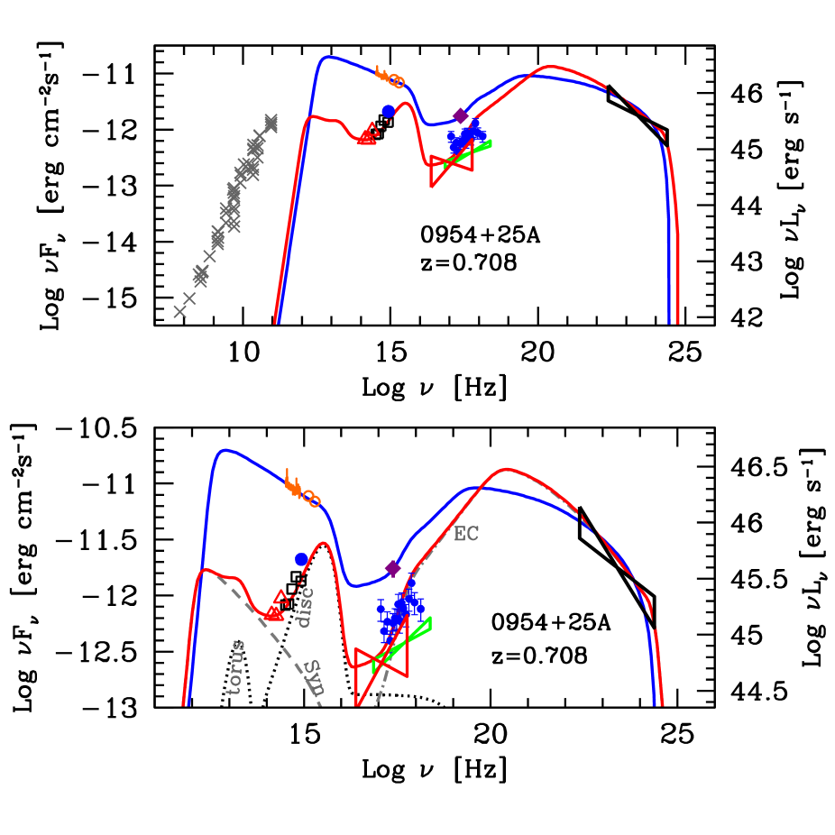
Figure 1: Broad band spectral energy distribution, and related models, of B2 0954+25A. Data are provided by several facilities (see §2.1). Upper panel shows all available data, from radio to $\gamma$–ray energies, as well as the SED models in the low and high synchrotron state. The lower panel shows a detailed view of the SED from IR to $\gamma$–rays, and highlights the most important components of the models.

Table 2: Observation dates for all data used to build the SED in Fig. 1.

Facility	Date of obs.
Einstein	1979–11–06
INT	1987–12–16
2MASS	1998–11–30
SDSS (photometry)	2004–12–13
SDSS (spectrum)	2006–01–05
GALEX	2006–02–05
Swift	2007–06–01
Chandra	2009–01–20
Fermi (average)	Aug 2008 – Jun 2011

Fermi/LAT — The 2LAC catalog (Ackermann et al., 2011) reports a flux for the source of $(2.1\pm 0.2)\times 10^{-12}$ erg s^-1 cm^-2 at 618 MeV, and a photon index $\Gamma=-2.39\pm 0.08$. We also ran a likelihood analysis on the first 34 months of data collected by Fermi/LAT (using ScienceTools ver. 9.23.1 and Instrument Response Function P6_V3) with time bins of one month, to check for the occurrence of major flares. We found no significant variability of the flux nor of the spectral index, i.e. a constant flux and spectral index model fits well observational data and cannot be rejected on statistical basis. The flux in the 0.1–100 GeV band averaged over 34 months is compatible with the value reported in 2LAC.

Swift/XRT — On June 1st, 2007 Swift performed a pointed observation (obsID 00036325002) of a nearby source, thus it has been possible to extract data for B2 0954+25A. We extracted a spectrum using the xrtpipeline script and binned it to have at least 20 counts in each bin. Then we used XSPEC to fit a simple power law with the hydrogen column fixed to the Galactic value $N_{\rm H}=3.2\times 10^{20}$ cm^-2. The resulting de–absorbed flux in the 0.3–10 keV energy band is $(2.5\pm 0.3)\times 10^{-12}$ erg cm^-2 s^-1and the photon index is $\Gamma=1.74\pm 0.09$.

Chandra — On June 20th, 2009 Chandra pointed our source. We extracted a spectrum using the specextract script, with a minimum of 30 counts in each bin, then performed a fit against a simple power law using Sherpa. Again the $N_{\rm H}$ column has been kept fixed to $3.2\times 10^{20}$ cm^-2. The resulting de–absorbed flux in the 0.3–10 keV energy band is $(1.32\pm 0.06)\times 10^{-12}$ erg cm^-2 s^-1and the photon index is $\Gamma=1.75\pm 0.07$.

GALEX — on Feb 5th, 2006 GALEX observed the source and provided the following photometric measurements: $(269\pm 18)$ $\mu$Jy at 1528 Å (far UV) and $(535\pm 14)$ $\mu$Jy at 2271 Å (near UV). Using a colour excess E(B–V) = 0.0377 we computed the de–reddened fluxes using CCM 1989 parametrization (Cardelli et al., 1989). The resulting $\nu F_{\nu}$ values are $(7.00\pm 0.47)\times 10^{-12}$ erg cm^-2 s^-1(FUV) and $(9.71\pm 0.26)\times 10^{-12}$ erg cm^-2 s^-1(NUV).

Swift/UVOT — An aperture photometry analysis of the $u$ filter data provided a count rate of 3.16 $\pm 0.11$ s^-1. The corresponding (Poole et al., 2008) de–reddened (Cardelli et al., 1989) $\nu F_{\nu}$ flux at 3501 Å is $(2.14\pm 0.07)\times 10^{-12}$ erg cm^-2 s^-1.

SDSS — Our source has been observed photometrically (Dec. 2004) and spectroscopically (Jan. 2006, see also §4) by SDSS. Both data sets have been de-reddened using Cardelli et al. (1989).

2MASS — An IR observation of the source has been performed on Nov 30th, 1998 and results are available in the 2MASS catalog. Magnitudes are $m_{J}=16.53\pm 0.13$, $m_{H}=16.12\pm 0.19$ and $m_{K}=15.34\pm 0.14$. The corresponding $\nu F_{\nu}$ fluxes are: $(9.5\pm 1.1)\times 10^{-13}$ erg cm^-2 s^-1at a 1.2 $\mu$m (J band), $(6.6\pm 1.1)\times 10^{-13}$ erg cm^-2 s^-1at a 1.6 $\mu$m (H band) and $(6.8\pm 0.8)\times 10^{-13}$ erg cm^-2 s^-1at a 2.2 $\mu$m (K band).

The broad band SED (built using archival data from facilities described in §2.1) is shown in Fig. 1. Grey crosses are from radio facilities, black squares are from Sloan photometry, red butterfly is from ROSAT, purple diamond is from Einstein. We added the data from Fermi/Large Area Telescope (LAT, black butterflies), Swift/X–Ray Telescope (XRT, blue dots), Chandra (green butterfly), GALEX (orange open circles), Swift/UltraViolet Optical Telescope (UVOT) (blue circles) and 2MASS (red triangles). Colors of simultaneous observations (Swift/XRT and UVOT, SDSS spectroscopic and GALEX) are the same. Looking at the SED in optical/UV it is clear that the source raised its flux by a factor $\sim$10 in about one year. In June 2007 the source returned to a lower state (in optical/UV) as shown by the Swift/UVOT measurements. Thus, the source shows at least a “low” and a “high” state in optical/UV. A similar trend, although of smaller magnitude, is shown at X–ray wavelengths with the lowest flux being measured by ROSAT and the highest being measured by Einstein.

In the following sections we will focus on specific wavelengths range, namely radio (§3) and optical (§4), and then provide an overall picture of the broad band SED (§5).

3 Radio properties

B2 0954+25A shows a flat radio spectrum from $\sim 10^{8}$ Hz to $\sim 10^{11}$ Hz. At 5 GHz, the luminosity of the core is log($L_{\rm c}$/erg s^-1 Hz^-1) = 34.5, while that of the extended region is log($L_{\rm e}$/erg s^-1 Hz^-1) = 32.4, thus the source is highly core–dominated with a core dominance parameter $R_{\rm cd}\sim 100$, i.e. at the higher end of the core–dominance parameter distribution (Browne & Murphy, 1987). The weakness of the extended emission is also evident at low radio frequencies, because the radio spectrum remains flat down to 74 MHz, with a spectral index $\alpha\sim-0.2$ between 74 and 365 MHz ($F_{\nu}\propto\nu^{\alpha}$). Assuming a spectral index for the optically thin emission in the extended region of –0.7, and extrapolating the flux from 5 GHz, the frequency at which the isotropic and the beamed jet luminosities are equal is $\sim$10 MHz, in agreement with the observed overall flat radio spectral index. This suggests that the jet is well aligned along the line of sight.

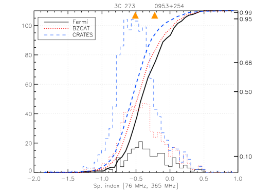
Figure 2: Distribution of spectral index between the (observed) frequencies 74 and 365 MHz for three different blazar catalogs: CRATES (Healey et al., 2007, blue dashed line), BZCAT (Massaro et al., 2009, red dotted line) and Fermi 2yr catalog of AGN (Ackermann et al., 2011, 2LAC, black solid line). Thicker lines show cumulative fraction (values on right axis). Radio fluxes to compute the spectral index are taken from the VLA survey at 74 MHz (Cohen et al., 2007) and the Texas survey at 365 MHz (Douglas et al., 1996).

We can compare the 74–365 MHz radio spectral index $\alpha$ of B2 0954+25A with the distribution of the same spectral index of other blazars. To this aim we show in Fig. 2 the distribution of spectral index between the (observed) frequencies 74 and 365 MHz for three different blazar catalogs: CRATES (Healey et al., 2007, blue line), BZCAT (Massaro et al., 2009, red line) and Fermi 2yr source catalog of AGN (2LAC, all “CLEAN” sources, Ackermann et al., 2011, black line). The radio fluxes to compute the spectral index are taken from the VLA survey at 74 MHz (Cohen et al., 2007) and the Texas survey at 365 MHz (Douglas et al., 1996). The number of sources detected at both frequencies is 1282 for the CRATES catalog; 605 for the BZCAT and 218 for the Fermi 2LAC catalog. The distribution shows that only $\sim$30% of the highly beamed blazars detected by Fermi have a steep ($\alpha<-0.5$) spectral index between 74 and 365 MHz. Radio–selected blazars from CRATES show a broader distribution with $\sim$50% sources having spectral index $<$–0.5. The BZCAT distribution is similar to CRATES, although with a larger fraction of very flat or inverted radio sources.

The extended region of B2 0954+25A, as observed in the 1.64 GHz VLA radio map, has a projected size of $\sim$50 kpc (Murphy et al., 1993; Liu & Zhang, 2002). This is rather large, especially considering that the viewing angle $\theta_{\rm v}$ is small, as suggested by the observed superluminal motion (12$c$, Kellermann et al., 2004) and by the SED modeling (§3.5 and Tab. 5). Assuming $\theta_{\rm v}$ in the range 3–6 degrees, the de–projected size is then in the range 0.5–1 Mpc, typically the size of a giant radio lobe.

We conclude that the radio properties of B2 0954+25A indicate a highly core dominated source, with an extended component that, albeit reaching the dimension of a giant radio lobe, is rather weak, making the core dominance parameter very large, at the high end of the distribution values for blazars.

4 Optical spectroscopy

We used optical spectra from the Isaac Newton Telescope (INT) and from SDSS (see Fig. 3). The spectrum from INT (observed on 16th Dec. 1987) has been derived directly from the plot given in Jackson & Browne (1991, their Fig. 2), thus it is suitable only for a qualitative analysis. The spectrum from SDSS (observed on 5th Jan. 2006) has been automatically flux– and wavelength–calibrated by the SDSS pipeline (Stoughton et al., 2002), de–reddened using Cardelli et al. (1989) with E(B–V)=0.0375 (Schlegel et al., 1998), transformed to rest frame of reference using our redshift estimate ($z$=0.70747, §4.1) and rebinned by a factor of 2 (Fig. 3, see Fig. 5 for a closer view of the H$\beta$ and [OIII] region).

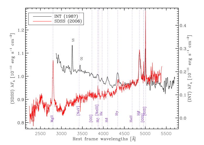
Figure 3: Optical spectrum of B2 0954+25A observed by SDSS in 2006 (red line, flux scale on the left axis) and with the Isaac Newton Telescope (INT) in 1987 (black line, flux scale on the right axis). The range of values covered by both axes is exactly the same ($\sim 0.5\times 10^{-11}$ erg s^-1 cm^-2) so that spectra can be directly compared. SDSS spectrum have been de–reddened using Cardelli et al. (1989) with E(B–V)=0.0375, transformed to the rest frame using our redshift estimate ($z$=0.70747, see text) and rebinned by a factor of 2. The INT spectrum has been derived from the plot given in Jackson & Browne (1991, their Fig. 2) and transformed to rest frame. The “S” letter denote a telluric line. Some of the most important emission lines are highlighted. The spectra show that the continuum has changed both in intensity (by a factor $\sim$5) and in slope. The intensity and shape of the Balmer lines seem to be the same in both spectra.

Figure 4: Profiles of MgII (2800Å), H$\beta$ (4863Å) and [OIII] (5007Å) emission lines in velocity offset space. Spectrum has been continuum–subtracted, the continuum level has been estimated by eye and all profiles have been normalized to have maximum of 1. Finally, profiles have been smoothed by a $\sim$4 Å boxcar average to provide a clearer view. Dashed lines allow to roughly measure full width at half maximum (FWHM) of each line.

Fig. 4 shows the profiles of the main emission lines, namely MgII (2800Å), H$\beta$ (4863Å) and [OIII] (5007Å), in velocity space. The spectrum has been continuum–subtracted and all profiles have been normalized to have maximum of 1. Finally all profiles have been smoothed by a $\sim$4 Å boxcar average to provide a clearer view. The dashed lines allow to approximately measure the full width at half maximum (FWHM) of each line.

To provide a better estimate of the FWHM of the H$\beta$ and [OIII] line profiles we also performed a fit of the spectrum using five components model (Model 1): a power–law to account for the continuum emission, four Gaussian–shaped emission lines to account for the H$\beta$ (both narrow and broad component) and the [OIII] 4959Å, [OIII] 5007Å lines. FWHM and velocity offset of the narrow lines are forced to be the same. Results are shown in Fig. 5 (upper panel). To account for residuals in the 4830 – 4900Å range (i.e. the asymmetry in the broad H$\beta$ line) we ran another fit by adding another emission line component named H$\beta^{*}$ (Model 2, Fig. 5 lower panel).

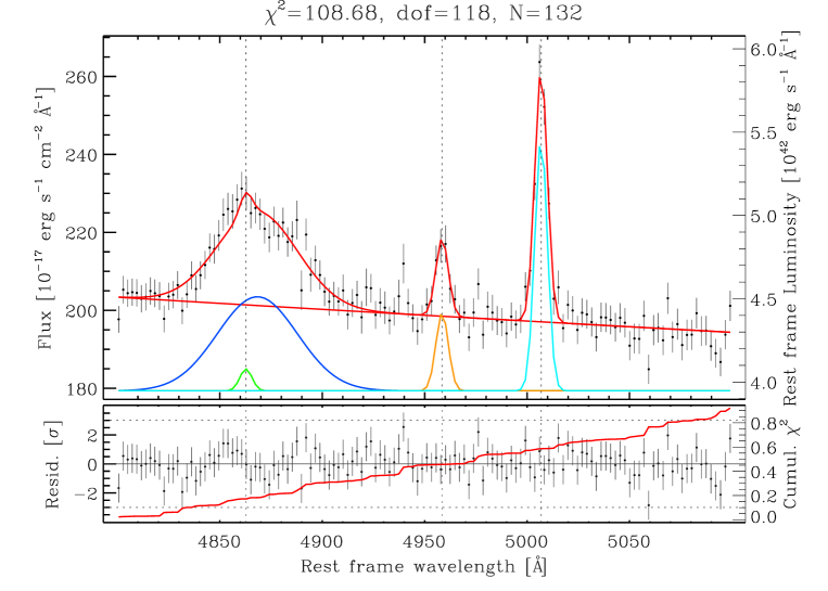
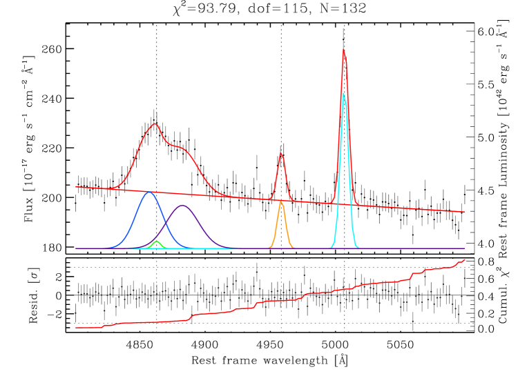
Figure 5: Spectrum of B2 0954+25A and fitted model in the range 4810–5100 Å. All quantities are quoted in rest frame. Upper panel: spectrum (black points, 1$\sigma$ error bars) with fitted model (red points) and model components: broad lines (red solid line), narrow lines (blue solid lines) and power–law continuum (green solid line). The broad and narrow lines components are shifted upward for clarity. The five black dotted lines are the rest line centers of (from left to right) H$\gamma$, H$\beta$, “line 2” (see text), [OIII] 4959 and [OIII] 5007 respectively. Red and blue dotted lines are the rest line centers of all broad and narrow considered lines. Lower panel: residual in units of one standard deviation. Red solid line is the cumulative reduced chi–squared (values on right axis).

4.1 Results

A qualitative comparison of the spectra by INT and SDSS taken $\sim$9 years apart (Tab. 2) shows that the continuum has changed both in intensity (by a factor $\sim$5) and in slope. The intensity and shape of the Balmer line seem to be the same in both spectra. In §2.1 we also analyze the broad–band SED (lower panel of Fig. 1) of the source, considering also the photometric data from SDSS, taken $\sim$1 year before the SDSS spectroscopic observations. Again, we see that a change in intensity of the optical emission of a factor $\sim$10 occurred in just 1 year. Also, a change in slope occurred, as indicated by the photometric data in the 5 available bands. Thus, we conclude that B2 0954+25A has been observed in at least three emission states at optical wavelengths, which differs in intensity: from the dimmer one (SDSS/photometric), through an intermediate one (INT), to the brighter one (SDSS/spectroscopic). The spectral slope is correlated to the change of state. As discussed in §5.2, the change of state can be simply explained as a change of magnetic field. A change in accretion rate is not needed, therefore we do not expect any change in line luminosity and profile. We will refer to these optical emission states as the disk dominated one, the intermediate state and the jet dominated state respectively, and discuss their properties in §5.2.

A quantitative spectral analysis can only be performed on the SDSS spectrum. Fig. 4 clearly shows that our value of $z$=0.70747 locates the peak of the [OIII] line exactly at 0 in velocity space, while the MgII peak is redshifted by $\sim$300 km s^-1 and the H$\beta$ peak is blueshifted by $\sim$100 km s^-1. Also, the H$\beta$ profile shows a pronounced asymmetry on the red wing. Rough estimates of the FWHMs are: 3050 km s^-1 for the MgII line, 2600 km s^-1 for the H$\beta$ line and $\sim$480 km s^-1 for the [OIII] line.

To provide better estimates of luminosities, widths and offsets of emission lines, and eventually highlight some peculiarities in the spectrum, we performed a fit with the models described above. The spectrum in the 4800 – 5100Å region, as well as the fitting model and the single components, are shown in Fig. 5 (Model 1 in upper panel, Model 2 in lower panel). Results are shown in Tab. 3.

Model 1: The resulting FWHM for the H$\beta$ line is $(2830\pm 220)$ km s^-1, while the FWHM of the narrow lines is $(430\pm 24)$ km s^-1, grossly consistent with the rough estimates obtained with Fig. 4. The model fits reasonably well the spectrum, and the $\chi^{2}$ value is rather small. Also, the luminosity of the continuum at 5100Å and the spectral slope, as well as the sum of luminosities from broad and narrow H$\beta$ lines and [OIII] luminosities, are consistent with the fit performed in S10 (Tab. 3), thus our model does not suffer from lack of iron line modeling (which is present in their fit). The value of FWHM and velocity offset for both the broad and narrow components of H$\beta$ are however, quite different. The strong discrepancies in FWHM between our results and those from S10 are probably due to the fact that we had the opportunity to carefully check the results of the fit, while in S10 an automatic fitting pipeline had to be used to handle the many spectra contained in the catalog.

Model 2: The residuals of the fit in Model 1 (Fig. 5, upper panel) look random everywhere, except in two regions: 4840–4900Å and 4930–4945Å, in which the residuals are quite “coherent”, suggesting the presence of further components. Although the model is far from being rejected ($\chi^{2}_{\rm red}<1$) these residuals are due to the asymmetry in the broad H$\beta$ profile discussed above, and to an additional emission line. Thus, we ran again the fit with a new broad H$\beta$–like component, named H$\beta^{*}$ in Tab. 3 (actually we are not interested in the additional line at 4940Å). Results are shown in Fig. 5 (lower panel) and Tab. 3. The extra component accounts well for the asymmetry of the H$\beta$ profile, and the residuals in the region now look random. The same consideration as for Model 1 applies for the luminosity and slope of the continuum, and the luminosity of the H$\beta$ and [OIII] lines. Clearly, the putative broad H$\beta$ line is now much narrower ($\sim$1500 km s^-1). Furthermore, the new H$\beta^{*}$ component has the same FWHM and velocity offset as the broad H$\beta$ values given in S10. This provides a possible explanation for the discrepancies between our results and those from S10.

Table 3: Quantities derived from fit parameters and corresponding quantities in the Shen et al. (2010) catalog.

Parameter	Model 1		Model 2		S10		Units
Lum. (H$\beta_{\rm broad}$)	26.3 $\pm$	2.2	12.9 $\pm$	6.3	23 $\pm$	13	[1042 erg s-1]
Lum. (H$\beta^{*}$)	—		12.1 $\pm$	5.8	—		[1042 erg s-1]
Lum. (H$\beta_{\rm narrow}$)	0.93 $\pm$	0.58	0.50 $\pm$	0.92	8 $\pm$	42	[1042 erg s-1]
Lum. ([OIII], 5007)	11.07 $\pm$	0.59	11.01 $\pm$	0.58	12.2 $\pm$	1.9	[1042 erg s-1]
FWHM (H$\beta_{\rm broad}$)	2830 $\pm$	220	1470 $\pm$	320	1870 $\pm$	600	[km s-1]
FWHM (H$\beta^{*}$)	—		1790 $\pm$	600	—		[km s-1]
FWHM (H$\beta_{\rm narrow}$)	431 $\pm$	24	428 $\pm$	24	1200 $\pm$	400	[km s-1]
Voff (H$\beta_{\rm broad}$)	344 $\pm$	75	–(350 $\pm$	270)	–(1250 $\pm$	630)	[km s-1]
Voff (H$\beta^{*}$)	—		1220 $\pm$	400	—		[km s-1]
Voff (H$\beta_{\rm narrow}$)	–(0 $\pm$	10)	1 $\pm$	10	37 $\pm$	200	[km s-1]
$\lambda$Lλ (5100Å)	220.88 $\pm$	0.80	220.59 $\pm$	0.78	220.73 $\pm$	0.74	[1044 erg s-1]
Continuum index	–(0.75 $\pm$	0.13)	–(0.85 $\pm$	0.11)	–(0.709 $\pm$	0.018)

In summary, our Model 2 seems to be the best description of the spectrum of B2 0954+25A in the 4810 – 5100 Å range.

4.2 The H$\beta$ line profile

The FWHM value of the H$\beta$ line profile reported in literature is 65 Å (Jackson & Browne, 1991). As shown in Tab. 4 the FWHM found with both Model 1 and 2 of our fit is significantly lower (46 Å and 24 Å respectively). Since the H$\beta$ profiles observed with INT and SDSS (Fig. 3) overlap perfectly, we can exclude a variation in the line profile, and conclude that previous value was likely overestimated. Moreover, the value reported in S10 is perfectly compatible with our estimate in Model 1 (48 Å, Tab.4).

Fig. 5 show that the broad H$\beta$ emission line can hardly be modeled with a single Gaussian profile, nor with any symmetric line profile such as the often quoted logarithmic profile (Blumenthal & Mathews, 1975), since the red wing is highly asymmetric. Iron emission lines in the range 4840–4900 Å are usually much weaker than the Balmer lines (Capriotti et al., 1979), thus such profile is hardly the result of a blending of different lines. Iron lines may be present but their intensity is negligible, indeed our fitting procedure provide the same results for line luminosities and width of narrow lines as reported in S10 (§4.1). Asymmetric H$\beta$ line profiles are not new in Type 1 AGN spectra: both red and blue asymmetries has been observed in all kind of AGNs (e.g. Capriotti et al., 1979, 1980; Peterson et al., 1987; Stirpe, 1990; Romano et al., 1996; Véron-Cetty et al., 2001), as well as profile variability (Osterbrock & Phillips, 1977; Peterson, 1987; Stirpe et al., 1988). Several kinematic models have been proposed to explain such features in the broad Balmer spectra of AGN, including radial inflow or outflow, different geometries and multiple components BLR (e.g. Peterson, 1987; Popović et al., 2004; Romano et al., 1996; Zhu et al., 2009), but no one has yet reached a general consensus. This hints for the presence of non virialized components in the BLR region. Thus, measures of FWHM performed on such profiles may not be directly related to the underlying black hole mass. This is the reason why we used the FWHM of just the main H$\beta$ line to estimate the virial black hole mass, neglecting the additional H$\beta^{*}$ component which account for the asymmetry. Doing so, the FWHM of H$\beta$ turns out to be about half the FWHM of MgII (Fig. 4). Such differences are common in sources with small values of FWHM(H$\beta$): in the S10 catalog, the MgII line is wider than H$\beta$ for $\sim$84% of the sources with FWHM(H$\beta$)$<2000$, and only 22% of the sources with FWHM(H$\beta$)$>4000$.

Of course the reasoning can be inverted: the “real” H$\beta$ line profile may be much wider, but some intervening gas could absorb radiation only on the blue side. Although we have no evidence to exclude this hypothesis, the range of values for the black hole mass found in §4.3 marginally supports the hypothesis that the real virialized line profile is the one modeled with the main H$\beta$ component. This conclusion may have important consequences on the classification of B2 0954+25A. Should the additional H$\beta^{*}$ component vanish in future observations, the FWHM of the remaining, virialized, H$\beta$ component would be $\sim$1500 km s^-1, and the source would become a powerful $\gamma$-RL-NLS1. (Foschini et al., 2009; Abdo et al., 2009c; Calderone et al., 2011). Such variations in line profiles have already been observed, on timescales of tens of years in NGC 5548 (Peterson, 1987).

4.3 Spectroscopically derived quantities

Spectroscopic measurements, such as those derived in §4.1, are used to infer some physical properties of the source, such as the total accretion luminosity $L_{\rm bol}$ and the virial black hole mass. The former is obtained by scaling the luminosity of one emission line (e.g. H$\beta$) to obtain the total BLR luminosity, $L_{\rm BLR}$, through a template quasar spectrum (Francis et al., 1991). $L_{\rm bol}$ can then be computed by dividing $L_{\rm BLR}$ by the covering factor, assumed to be 0.1. Black hole masses are usually estimated assuming virialized motion of BLR clouds. The BLR radius has been measured by means of the reverberation mapping technique (RM, Peterson, 1993) for a few tens of objects, and a correlation between the continuum optical luminosity and the BLR size, has been calibrated ($R$–$L$ relation, Kaspi et al., 2005; Vestergaard & Peterson, 2006; Bentz et al., 2009), so that we can infer $R_{\rm BLR}$ size without the (very time–consuming) RM observational campaigns. Thus, it is in principle possible to estimate black hole masses using single–epoch optical spectroscopy (such as the SDSS spectrum of B2 0954+25A used in §4) and a calibrated virial mass scaling relationship (such as those reported in Vestergaard & Peterson (2006)). There are, however, several caveats, such as the geometry and orientation of the BLR (Decarli et al., 2011), the role of radiation pressure (Marconi et al., 2008, 2009) and the way line profiles should be analyzed to infer the orbital velocity of the clouds. Indeed, the H$\beta$ broad line is often asymmetric, thus the broadening cannot be simply interpreted as being due to orbital bulk motion. In these cases is not clear what measure should be taken for the line width. Note also that RM studies have been carried out mainly on radio–quiet sources, i.e. sources in which synchrotron emission from a jet at optical/IR wavelengths is negligible with respect to the emission from the so called Big Blue Bump (BBB). Thus, the $R$–$L$ relations are reliable only when the BBB is clearly visible (Wu et al., 2004). Contribution from host starlight is also supposed to be an issue (e.g. Bentz et al., 2009), although only in low luminosity AGN (log($\lambda L_{\lambda}$,5100Å)$<$44.5, Shen et al., 2010), therefore not in the case of B2 0954+25A. Finally, the 1$\sigma$ statistical dispersion of virial mass scaling relationships against RM–based masses is estimated to be $\sim$0.5 dex. The RM masses are in turn scattered by the same factor around the $M$–$\sigma$ relation (Onken et al., 2004). The absolute accuracy is therefore estimated to be of the order of 0.7 dex (Vestergaard & Peterson, 2006).

We will consider virial mass estimates computed using both Model 1 and 2. Also, the SDSS spectrum of B2 0954+25A has been taken when the source was in the jet dominated state, therefore we cannot use the continuum luminosity estimated from spectral analysis to infer the BLR size. Instead, we will use optical data of the disk dominated state, as observed photometrically by SDSS.

4.3.1 Results

To compute $L_{\rm BLR}$, and the disk bolometric luminosity $L_{\rm bol}$, we use the composite quasar spectrum given in Francis et al. (1991), including the H$\alpha$ contribution as in Celotti et al. (1997). The broad H$\beta$ line contributes to the entire $L_{\rm BLR}$ with a weight 22/555 (the Ly$\alpha$ contributes for 100/555). Using the luminosity of the H$\beta$ complex found with Model 2 fitting (broad H$\beta$ line + H$\beta^{*}$ component, log($L$(H$\beta$)/erg s^-1) = 43.4), and setting $L_{\rm bol}=10L_{\rm BLR}$, we estimate log($L_{\rm bol}$/erg s^-1) = 45.8. This value agrees with the one derived in §5 through SED modeling: log($L_{\rm bol}$/erg s^-1) = 46. Instead, S10 reports log($L_{\rm bol}$/erg s^-1) = 47, because S10 used an observation made when the source was in the jet dominated state.

Table 4: Black hole mass estimates using different methods and calibrations. Continuum luminosity at 3000Å and 5100Å (rest frame) used in virial estimates are log($\nu L_{\nu}$/erg s^-1) = 45.7 and 45.3 for MgII and H$\beta$ respectively (derived from SDSS photometry). Col. [1]: method used; Col. [2]: reference for the FWHM of the emission line; Col. [3]: FWHM of the broad emission line; Col. [4]: black hole mass estimate; Col. [5]: Eddington ratio, assuming a bolometric luminosity log($L_{\rm bol}$/erg s^-1) = 45.95 (see §5 and Tab. 5); Col. [6]: calibration references: (a) Shen et al. (2010), (b) Vestergaard & Osmer (2009), (c) Vestergaard & Peterson (2006), (d) Bentz et al. (2009), (e) Tremaine et al. (2002).

Method	FWHM ref.	FWHM [km s-1, (Å)]	log M/M☉	Edd. ratio	Calib. ref.
[1]	[2]	[3]	[4]	[5]	[6]
Virial, MgII	S10, broad comp.	3980 ( 65 )	9.0	0.1	(a)
	S10, whole profile	3390 ( 55 )	8.8	0.1	(b)
Virial, H$\beta$, single comp.	S10	2970 ( 48 )	8.6	0.2	(c)
	Model 1	2830 ( 46 )	8.5	0.3	(d)
Virial, H$\beta$, H$\beta^{*}$	Model 2	1470 ( 24 )	7.9	1.1	(d)
M-$\sigma_{*}$ ([OIII])	Model 2	430 ( 7 )	8.0	0.9	(e)
SED modeling	—	—	8.2	0.6

Tab. 4 reports the black hole mass estimates for B2 0954+25A obtained using different methods and calibrations. For all estimates, except the last two, we used the virial mass scaling relations. The first two estimates are computed using the FWHM estimates (of the broad component and the whole profile respectively) of the MgII emission line provided by S10, the continuum luminosity derived from SDSS photometry (when the source was in the disk dominated state) of log($\nu L_{\nu}$/erg s^-1) = 45.7 and the same calibrations used in S10: Shen et al. (2010) and Vestergaard & Osmer (2009) respectively. The mass estimates are very similar, so we will refer to them as the MgII virial mass estimates (log $M/M_{\sun}\sim 9$).

The next two estimates are computed using the FWHM of the H$\beta$ emission line fitted with a single Gaussian. Values for FWHM are provided by S10 and by our Model 1 respectively, the continuum luminosity is derived from SDSS photometry (disk dominated state): log($\nu L_{\nu}$/erg s^-1) = 45.3, and the calibration are from Vestergaard & Peterson (2006, same as S10) and Bentz et al. (2009), respectively. This pair of mass estimates are also very similar, so we will refer to them as the single H$\beta$ virial mass estimates (log $M/M_{\sun}\sim 8.5$).

Next estimate is computed using the FWHM of the H$\beta$ emission line from Model 2, neglecting the additional H$\beta^{*}$ component, and the calibration by Bentz et al. (2009).

Finally, the last two rows of Tab. 4 report mass estimates obtained without using the virial method. For the first one we used the FWHM of the [OIII] line (provided by Model 2 fitting) as a proxy for the stellar velocity dispersion, and the calibration of the $M-\sigma_{*}$ relation given in Tremaine et al. (2002, their Eq. 20). Updated calibration given in Graham et al. (2011) produces the same result. In the last one we simply report the mass estimate obtained in §5 through SED modeling. Notice that the last three methods yield very similar results (log $M/M_{\sun}\sim 8$), even if they have been derived using different and independent methods.

4.3.2 Discussion

Our black hole mass estimates are considerably lower than those found in the literature (§2). This is likely a consequence of the different values of the H$\beta$ line profile’s width, as discussed in 4.2. Also, the mass given in S10 is probably overestimated since the continuum luminosity has been measured while the source was in the jet dominated state. Therefore, we will consider only our mass estimates given in Tab. 4.

In particular, the estimate obtained with Model 2 (neglecting the H$\beta^{*}$ component), and the $M$-$\sigma$ relation (log($M/M_{\sun}$) $\sim$8) are quite independent, thus they provide greater confidence about the goodness of the mass estimate. Modeling the disk dominated state with a standard (i.e. Shakura & Sunyaev, 1973) disk (§5.2) yields estimates of the black hole mass between $(1.5-5)\times 10^{8}M_{\odot}$. Smaller masses are excluded because the disk would become super–Eddington, larger masses are excluded because, beside providing a worse fit to the near–IR and optical data of the “disk–dominated” state, they require a smaller ionizing luminosity, that becomes incompatible with the luminosity of the broad line region. We therefore conclude that the black hole mass of B2 0954+25A is in the range log($M/M_{\sun}$) = 8–8.5.

5 Modeling the SED

To model the SED we use the one–zone leptonic model described in detail in Ghisellini & Tavecchio (2009), whose main characteristics are briefly described in the Appendix. The SED of the source is shown in Fig. 1. The lower panel shows a zoom of the optical, X–ray and $\gamma$–ray data part of the SED, together with the models used to interpret the two states of the source. As discussed above, SDSS observed B2 0954+25A in two occasions, approximately one year apart. In the first observation the SDSS made the photometry in its usual optical filters (black squares in Fig. 1), while the spectrum, one year later, revealed a very high state, dominated by the beamed synchrotron emission (orange lines), in agreement with the GALEX observations (orange open circles).

For the low optical state we have simultaneous UVOT and XRT Swift observations: the UVOT point (blue filled circle) agrees with the photometric SDSS data points (black squares) and with the 2MASS data (red triangles). We have then modeled these data together with the XRT X–ray data, assuming also that the average Fermi/LAT flux and spectrum is a good representation of the high energy emission of this state.

On the other hand we have no information about the level of the $\gamma$–ray flux for the high optical state of the source. We therefore assume that it corresponds also to a high state of the X–ray emission, that can be represented by the maximum X–ray flux observed (violet diamond point), and to the same $\gamma$–ray flux.

The Chandra and Fermi data shown as green/black ties are simultaneous (even if the Fermi spectrum is the average of 34 months of observations), but we do not have any information about the optical–UV state. During the 34 months of Fermi observations, the $\gamma$–ray flux was rather stable, with no sign of significant variability. The one–zone leptonic model (in which optical and $\gamma$–ray radiation are produced by the same population of electrons) is perfectly suitable to describe this SED. Detection of optical variability without corresponding changes in simultaneous $\gamma$–ray observations would be, however, difficult to accomodate in the framework of the one–zone leptonic model.

In Tab. 5 we list the relevant parameters used to interpret the two states of the source, namely the disk and the jet dominated one. Tab. 6 reports the jet powers corresponding to the two states, calculated as explained in the Appendix.

5.1 Guidelines for the choice of the parameters

Accretion disk — The luminosity of the accretion disk can be estimated through the luminosity of the broad emission lines $L_{\rm BLR}$, assuming a given value for the covering factor. As discussed in detail in §4.3, we can estimate $L_{\rm BLR}\sim 6.3\times 10^{44}$ erg s^-1. Assuming a covering factor of $\sim$0.1, the disk luminosity is of the order of $10^{46}$ erg s^-1. Given the uncertainties about $L_{\rm BLR}$, derived using only the $H\beta$ line, the covering factor and the mass of the black hole (controlling the $L_{\rm d}/L_{\rm ion}$ ratio), this estimate necessarily has an uncertainty of at least a factor 2.

Location of the emitting region — The SED in the low state shows that the high energy hump dominates the bolometric output, as in other powerful Flat Spectrum Radio Quasars (FSRQs). In these objects it is likely that the emitting region is located inside the BLR, since in these cases the seed photons produced by the BLR, whose flux is seen enhanced in the comoving frame of the emitting region, dominate the radiative cooling. We then assume $R_{\rm diss}<R_{\rm BLR}$, where $R_{\rm diss}$ is the distance of the emitting region from the black hole, and $R_{\rm BLR}\sim 10^{17}L_{\rm d,45}^{1/2}$ cm is the size of the BLR.

Magnetic field — The value of the magnetic field is chosen in order to reproduce the ratio between the synchrotron and the inverse Compton flux.

Bulk Lorentz factor — This has been chosen in order to reproduce the superluminal apparent velocity ($\beta_{\rm app}\sim 12$, Kellermann et al. 2004). This also fixes the viewing angle, that must be of the order of $1/\Gamma$. Note that the value of $\Gamma$ determines the value of the radiation energy density of the external seed photons ($\propto\Gamma^{2}$) and hence the value of the magnetic field required to have the observed synchrotron to inverse Compton luminosity ratio.

Injected power — The power is injected throughout the source in the form of relativistic electrons. Through the continuity equation we calculate the particle distribution as a result of injection, cooling and possible pair production. The total injected power is such that the radiation produced by these particles agrees with the observed data. The injected distribution is assumed to be a smoothly broken power law. The resulting distribution, modified by cooling, must agree with the observed slopes.

5.2 Results

The most notable feature of B2 0954+25A is the large variability in the optical, from a disk to a jet dominated emission. This is interpreted as a change in the magnetic field, from $\sim 5$ to 20 G, accompanied by an increase of the total injected power (by a factor 2), and a decrease in the maximum particles energy and a flattening of the high energy slope of the particle distribution. The location of the emitting region is somewhat less in the high optical state. We maintained the same bulk Lorentz factor. The power of the jet of B2 0954+25A carried by the magnetic field is larger in the high optical state (factor 10), while the differences in the other forms of power are minor. The jet power ($P_{\rm p}+P_{\rm e}$) is dominated by the bulk motion of protons. An electron to (cold) proton ratio of $\sim 1$ results in $P_{\rm p}\sim(2-5)\times 10^{47}$ erg. The jet power decreases by a factor of 20 if there are 20 electron–positron pairs per proton. Such a lepton to proton ratio is about the maximum allowed to make the jet not to recoil under the Compton drag effect (Ghisellini & Tavecchio, 2010). A value $P_{\rm p}\sim 2\times 10^{46}$ erg s^-1 makes the jet power similar to the accretion disk luminosity (which is slightly larger than $10^{46}$ erg s^-1). The minimum value of jet power is the one needed to produce the observed radiation, that is of the order of $P_{\rm r}\sim L_{\rm obs}/\Gamma^{2}$= (3–7)$\times 10^{44}$ erg s^-1. Even this absolute lower limit on the jet power contrasts with the absence of a strong extended emission (see §3). In fact, following Willott et al. (1999), we can estimate the jet power $Q$ from the extended luminosity at 151 MHz. Extrapolating from 5 GHz, assuming $F_{\nu}\propto\nu^{-1}$, we derive $Q\sim 5\times 10^{43}$ erg s^-1, a value that is even smaller than $P_{\rm r}$.

These values of the physical parameters are similar to those found by fitting Fermi blazars (Ghisellini et al., 2010), with the black hole mass being in the low end of the distribution. We have used a black hole mass $M=1.5\times 10^{8}M_{\odot}$. We have also fitted the spectrum with larger black hole masses, and obtain equally good fits with $M=3\times 10^{8}M_{\odot}$ (and $L_{\rm d}/L_{\rm Edd}=0.34$) and $M=5\times 10^{8}M_{\odot}$ (and $L_{\rm d}/L_{\rm Edd}=0.17$). Both these alternative solutions are acceptable since they provide a sufficient $L_{\rm ion}$ to photoionize the BLR. If $M=10^{9}M_{\odot}$, instead, the computed disk emission shifts to smaller frequencies (i.e. the disk becomes colder) and then we are obliged to decrease its overall luminosity. As a consequence, we cannot reproduce the Swift/UVOT $u$ point, and the ionizing luminosity becomes too small to efficiently photoionize the BLR.

The picture that emerges is that of a typical Fermi blazar, with a flat radio spectrum produced by a powerful jet, and black hole mass significantly smaller than $10^{9}M_{\odot}$. The source periodically cycles through different emission states, characterized by different amount of power emitted by the jet. Although the SED parameters are only rough estimates of physical quantities, the possibility to model two different states of the same source provides at least a clue that the parameters kept fixed in both models (black hole mass, disk luminosity, BLR radius, covering factor) are reliable.

State	$R_{\rm diss}$	$M$	$L_{\rm d}$	$R_{\rm BLR}$	$P^{\prime}_{\rm i}$	$B$	$\Gamma$	$\theta_{\rm v}$	$\gamma_{\rm b}$	$\gamma_{\rm max}$	$s_{1}$	$s_{2}$	$\gamma_{\rm cool}$
[1]	[2]	[3]	[4]	[5]	[6]	[7]	[8]	[9]	[10]	[11]	[12]	[13]	[14]
jet dominated	45 (1000)	1.5e8	11.3 (0.58)	335	0.014	21	13	3	100	2.5e3	2	2.5	7
disk dominated	59 (1300)	1.5e8	11.3 (0.58)	335	7e–3	5.2	13	3	100	5e3	2	2.9	21
PMN J0948+0022	2 (1600)	1.5e8	9 (0.4)	300	0.024	3.4	10	6	800	1.6e3	1	2.2
3C 273	120 (500)	8e8	48 (0.4)	693	0.015	11.6	12.9	3	40	2e4	1	3.4

Table 5: Input parameters used to model the SED of B2 0954+25A (first two lines), PMN J0948+0022 and 3C 273 (Ghisellini et al., 2010). Col. [1]: State of the source; Col. [2]: distance of the blob from the black hole in units of $10^{15}$ cm and in units of the Schwarzschild radius; Col. [3]: black hole mass in solar masses; Col. [4]: Disk luminosity in units of $10^{45}$ erg s^-1 and in Eddington units; Col. [5]: distance of the BLR in units of $10^{15}$ cm; Col. [6]: power injected in the blob calculated in the comoving frame, in units of $10^{45}$ erg s^-1; Col. [7]: magnetic field in Gauss; Col. [8]: bulk Lorentz; Col. [9]: viewing angle in degrees; Col. [10], [11] and: minimum and maximum random Lorentz factors of the injected electrons; Col. [12] and [13]: slopes of the injected electron distribution [$Q(\gamma)$] below and above $\gamma_{\rm b}$; Col. [14] minimum random Lorentz factor of the electrons cooling in one light crossing time $R/c$. The disk has an X–ray corona of luminosity $L_{X}=0.3L_{\rm d}$. The spectral shape of the corona is assumed to be $\propto\nu^{-1}\exp(-h\nu/150~{}{\rm keV})$.

State	$\log P_{\rm r}$	$\log P_{\rm B}$	$\log P_{\rm e}$	$\log P_{\rm p}$	$\log(P_{\rm p}/20)$
jet domin.	44.81	45.75	44.92	47.71	46.41
disk domin.	44.56	44.77	44.71	47.41	46.11
0948+0022	45.30	44.35	44.71	46.68	45.38
3C 273	45.05	46.09	44.90	47.48	46.18

Table 6: Jet power in the form of radiation, Poynting flux, bulk motion of electrons and protons (assuming one cold proton per emitting electron and 20 pairs per proton) for of B2 0954+25A (first two lines), PMN J0948+0022 and 3C 273 (Ghisellini et al., 2010).

6 Comparison with 3C 273 and PMN J0948+0022

In Fig. 6 we compare the broad band SED of B2 0954+25A to that of 3C 273 (upper panel) and PMN J0948+0022 (lower panel). Both sources have been analyzed in Ghisellini et al. (2010) and model parameters are reported in Tab. 5 and 6. The radio spectrum of the prototypical blazar 3C 273 shows a flat spectrum comparable in luminosity with B2 0954+25A, although slightly steeper. At the lowest observed frequencies the two SED are markedly different: whereas the 74–365 MHz radio spectral index of 3C 273 become steep ($\alpha\sim-0.5$), the spectral index of B2 0954+25A remains flat ($\alpha\sim-0.2$). As discussed in §3, this behaviour can be explained with a different amount of relativistic beaming which boosts the jet emission in B2 0954+25A. At shorter wavelengths 3C 273 is $\sim$1 order of magnitude more powerful than B2 0954+25A. If emission in both sources occur at approximately the same Eddington ratio (0.4–0.6, Tab. 5) as suggested by SED modeling, the luminosity ratio at optical/UV wavelengths ($\sim$ 3) provides an estimate for the mass ratio. Since log($M/M_{\sun}$) of 3C 273 is 8.9, for B2 0954+25A we expect a mass of $\sim$8.4. This is yet another indication that the black hole mass of B2 0954+25A should be significantly smaller than log($M/M_{\sun})=9$.

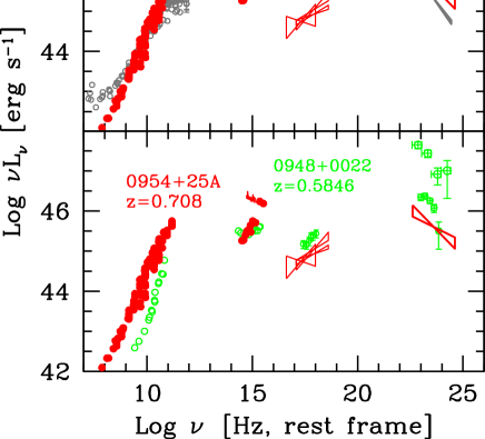
Figure 6: Comparison of the SED of B2 0954+25A with the SED of 3C 273 (top panel) and PMN J0948+0022 (bottom).

Also, the SED of PMN J0948+0022 is very similar to that of B2 0954+25A (in the disk dominated state), the only difference being at $\gamma$–rays (where PMN J0948+0022 showed an exceptional flaring episode (Foschini et al., 2011)). Parameters from the SED modeling and jet powers are quite similar (Tab. 5 and 6). This similarities support our speculation on the possible classification of B2 0954+25A as a $\gamma$–NLS1.

However, this similarity cannot be pushed too far, since B2 0954+25A lacks the strong iron emission that usually characterizes NLS1. Also, X–ray photon index of B2 0954+25Ais $\Gamma=1.74$ (§2.1), while that of NLS1 is typically $\Gamma>2.5$ (Boller et al., 1996). However, consider that also the other NLS1 detected by Fermi have a flat X–ray spectrum (Abdo et al., 2009b, c) likely because the flat X–ray jet emission dominates.

6.1 Typical Fermi blazar or $\gamma$-NLS1?

As discussed in §5 and §6, B2 0954+25A is a typical Fermi blazar. However, the likely small black hole mass of B2 0954+25A and the SED resemblance with prototypical $\gamma$–NLS1 PMN J0948+0022 suggest some similarities between the two sources. B2 0954+25A does not meet the commonly adopted classification criterion for NLS1, namely a FWHM of broad H$\beta<$2000 km s^-1 (Osterbrock & Pogge, 1985). However, the physical nature of such empirical threshold has been often questioned (e.g. Goodrich, 1989; Véron-Cetty et al., 2001) since all observational properties show a continuous transition at FWHM(H$\beta)\sim$2000 km s^-1, i.e. properties of NLS1 and BLS1 sources are smoothly joined.

Alternative criteria to distinguish among BLS1 and NLS1 sources have been put forward. Sulentic et al. (2000) proposed to increase the dividing threshold to 4000 km s^-1, to select radio–quiet sources with low mass and high accretion rate. Véron-Cetty et al. (2001) suggested to consider the strength of FeII emission relative to H$\beta$ as a possible tracer of the Eddington ratio. Netzer & Trakhtenbrot (2007) proposed to classify as narrow–line AGN (NLAGN) all sources exceeding an Eddington ratio of 0.25 (regardless of black hole mass).

A small black hole mass is likely a characterizing property of NLS1 sources (Grupe & Mathur, 2004). We would like to stress that if asymmetry in broad Balmer line profiles are due to non-virialized components in the BLR, then only the virialized one should be considered to estimate the black hole mass, and thus the NLS1 classification. In this case B2 0954+25A would be classified as a powerful $\gamma$–NLS1, just like PMN J0948+0022.

Since the overall properties of B2 0954+25A are similar to both classes of Fermi blazars and $\gamma$–NLS1, we conclude that it is one of those objects which smoothly joins the population of narrow–line and broad–line AGN.

7 Summary and conclusions

In this paper we carried out an extensive analysis on the Fermi blazar B2 0954+25A using archival data. We highlighted several peculiarities in the aim at providing a coherent picture of its physical properties. The main conclusions are as follows:

• (§2, §2) the source B2 0954+25A is a strong $\gamma$–ray emitter, detected both in the 1yr and 2yr Fermi/LAT point source catalogs (Abdo et al., 2010, 2011). We find no significant variability of the flux nor of the spectral index in the 0.1–100 GeV band in the first 34 months of data from Fermi/LAT.

• (§3) its radio spectrum is “flat” down to very low frequencies (74 MHz, Cohen et al., 2007), i.e. the optically thick synchrotron emission from the jet is dominating over the optically thin, isotropic emission from extended region. This observation indicates that the viewing angle must be small (3–6 degrees). The corresponding de–projected size of the jet is in the range 0.5–1 Mpc, the size of a giant radio lobe. The isotropic and the beamed components should have equal luminosities at $\sim$10 MHz.

• (§3, Fig. 2) the “flatness” of the radio spectrum at low frequencies observed in B2 0954+25A is typical of Fermi detected blazars (2LAC sample), i.e. well aligned blazars. Radio selected blazars show steeper spectra on average (e.g. the CRATES sample).

• (§4.1, Fig. 1 and 3) B2 0954+25A has been observed in at least three different optical states: from a disk–dominated state, to a jet dominated one in which the synchrotron emission overwhelms the emission from the disk, via an intermediate state. The two extreme states differ by nearly one order of magnitude in luminosity. Despite the change in continuum luminosity, the broad hydrogen Balmer lines maintain the same luminosity and line profile.

• (§4.1, Fig. 5, Tab. 3) the previously known estimate for the FWHM of the broad H$\beta$ line profile (65 Å rest frame, corresponding to $\sim$4000 km s^-1) from Jackson & Browne (1991) is probably overestimated. Also, the value of 1870 km s^-1 reported in Shen et al. (2010) is probably due to a poor model fit. A more likely value is 46 Å, corresponding to $\sim$2800 km s^-1. The broad H$\beta$ line shows a pronounced asymmetry on the red wing, which require a second Gaussian component (H$\beta^{*}$) of similar FWHM, to be modeled. The velocity offset of the H$\beta^{*}$ is $\sim$1200 km s^-1.

• (§4.1, Fig. 4) [OIII] 5007Å and MgII lines are quite symmetric. The FWHM of the MgII line is $\sim$ 3050 km s^-1, and the peak is redshifted by $\sim$300 km s^-1 with respect to the redshift identified by the [OIII] line.

• (§4.3, §4.3.2) the most likely value of the black hole mass is $M\sim(1-3)\times 10^{8}M_{\odot}$, as suggested by several independent methods. In particular, for the mass scaling relations we considered only the symmetric component of the H$\beta$ profile, and the continuum luminosity in the disk dominated state.

• (§5, Fig. 1, Tab. 5, §6) modeling the broad band spectral energy distribution, we derive physical parameters quite typical of other Fermi blazars.

• (§6) We suggest to classify B2 0954+25A as a transition object between the class of FSRQ and $\gamma$-NLS1, since it shows characteristic features of both classes (namely, the blazar appearance and the similarity with the SED of PMN J0948+0022).

Appendix A Appendix: Some details on the modeling

We use the model described in detail in Ghisellini & Tavecchio (2009). The emitting region is assumed spherical, at a distance $R_{\rm diss}$ from the black hole, of size $R=\psi R_{\rm diss}$ (with $\psi=0.1$), and moving with a bulk Lorentz factor $\Gamma$. The bolometric luminosity of the accretion disk is $L_{\rm d}$.

The energy particle distribution $N(\gamma)$ [cm^-3] is calculated solving the continuity equation where particle injection, radiative cooling and pair production (via the $\gamma$–$\gamma\to e^{\pm}$ process), are taken into account. The created pairs contribute to the emission. The injection function $Q(\gamma)$ [cm^-3 s^-1] is assumed to be a smoothly joining broken power–law, with a slope $Q(\gamma)\propto\gamma^{-{s_{1}}}$ and $\gamma^{-{s_{2}}}$ below and above a break energy $\gamma_{\rm b}$:

$$Q(\gamma)\,=\,Q_{0}\,{(\gamma/\gamma_{\rm b})^{-s_{1}}\over 1+(\gamma/\gamma_{\rm b})^{-s_{1}+s_{2}}}$$ (1)

The total power injected into the source in the form of relativistic electrons is $P^{\prime}_{\rm i}=m_{\rm e}c^{2}V\int Q(\gamma)\gamma d\gamma$, where $V=(4\pi/3)R^{3}$ is the volume of the emitting region.

The injection process lasts for a light crossing time $R/c$, and we calculate $N(\gamma)$ at this time. This assumption comes from the fact that even if injection lasted longer, adiabatic losses caused by the expansion of the source (which is traveling while emitting) and the corresponding decrease of the magnetic field would make the observed flux to decrease. Therefore the calculated spectra correspond to the maximum of a flaring episode.

Above and below the accretion disk, in its inner parts, there is an X–ray emitting corona of luminosity $L_{\rm X}$ (it is fixed at a level of 30% of $L_{\rm d}$). Its spectrum is a power law of energy index $\alpha_{X}=1$ ending with a exponential cut at $E_{\rm c}=$150 keV. The specific energy density (i.e. as a function of frequency) of the disk and the corona are calculated in the comoving frame of the emitting blob, and used to properly calculate the resulting External inverse Compton spectrum. The BLR is assumed to be a thin spherical shell, of radius $R_{\rm BLR}=10^{17}L_{\rm d,45}^{1/2}$ cm. We consider also the presence of a IR torus, at larger distances. The internally produced synchrotron emission is used to calculate the synchrotron self Compton (SSC) flux. Table 5 lists the adopted parameters.

Table 6 lists the power carried by the jet in the form of radiation ($P_{\rm r}$), magnetic field ($P_{\rm B}$), emitting electrons ($P_{\rm e}$, no cold electron component is assumed) and cold protons ($P_{\rm p}$, assuming one proton per emitting electron). All the powers are calculated as

$$P_{i}\,=\,\pi R^{2}\Gamma^{2}\beta c\,U^{\prime}_{i}$$ (2)

where $U^{\prime}_{i}$ is the energy density of the $i$ component, as measured in the comoving frame.

The power carried in the form of the produced radiation, $P_{\rm r}=\pi R^{2}\Gamma^{2}\beta c\,U^{\prime}_{\rm rad}$, can be re–written as [using $U^{\prime}_{\rm rad}=L^{\prime}/(4\pi R^{2}c)$]:

$$P_{\rm r}\,=\,L^{\prime}{\Gamma^{2}\over 4}\,=\,L{\Gamma^{2}\over 4\delta^{4}}\,\sim\,L{1\over 4\delta^{2}}$$ (3)

where $L$ is the total observed non–thermal luminosity ($L^{\prime}$ is in the comoving frame) and $U^{\prime}_{\rm rad}$ is the radiation energy density produced by the jet (i.e. excluding the external components). The last equality assumes $\theta_{\rm v}\sim 1/\Gamma$.

When calculating $P_{\rm e}$ (the jet power in bulk motion of emitting electrons) we include their average energy, i.e. $U^{\prime}_{\rm e}=n_{\rm e}\langle\gamma\rangle m_{\rm e}c^{2}$.

References

- Abazajian et al. (2009) Abazajian K. N., et al., 2009, ApJS, 182, 543
- Abdo et al. (2009a) Abdo A. A., et al., 2009a, ApJ, 699, 976
- Abdo et al. (2009b) Abdo A. A., et al., 2009b, ApJ, 707, 727
- Abdo et al. (2009c) Abdo A. A., et al., 2009c, ApJ, 707, L142
- Abdo et al. (2010) Abdo A. A., et al., 2010, ApJS, 188, 405
- Abdo et al. (2011) Abdo A. A., et al., 2011, (arXiv:1108.1435)
- Ackermann et al. (2011) Ackermann M., et al., 2011, ApJ, 743, 171
- Bentz et al. (2009) Bentz M. C., Peterson B. M., Netzer H., Pogge R. W., Vestergaard M., 2009, ApJ, 697, 160
- Blumenthal & Mathews (1975) Blumenthal G. R., Mathews W. G., 1975, ApJ, 198, 517
- Boller et al. (1996) Boller T., Brandt W. N., Fink H., 1996, A&A, 305, 53
- Browne & Murphy (1987) Browne I. W. A., Murphy D. W., 1987, MNRAS, 226, 601
- Burbidge & Strittmatter (1972) Burbidge E. M., Strittmatter P. A., 1972, ApJ, 174, L57+
- Calderone et al. (2011) Calderone G., Foschini L., Ghisellini G., Colpi M., Maraschi L., Tavecchio F., Decarli R., Tagliaferri G., 2011, MNRAS, 413, 2365
- Capriotti et al. (1979) Capriotti E., Foltz C., Byard P., 1979, ApJ, 230, 681
- Capriotti et al. (1980) Capriotti E., Foltz C., Byard P., 1980, ApJ, 241, 903
- Cardelli et al. (1989) Cardelli J. A., Clayton G. C., Mathis J. S., 1989, ApJ, 345, 245
- Celotti et al. (1997) Celotti A., Padovani P., Ghisellini G., 1997, MNRAS, 286, 415
- Cohen et al. (2007) Cohen A. S., Lane W. M., Cotton W. D., Kassim N. E., Lazio T. J. W., Perley R. A., Condon J. J., Erickson W. C., 2007, AJ, 134, 1245
- Decarli et al. (2011) Decarli R., Dotti M., Treves A., 2011, MNRAS, 413, 39
- Douglas et al. (1996) Douglas J. N., Bash F. N., Bozyan F. A., Torrence G. W., Wolfe C., 1996, AJ, 111, 1945
- Foschini (2011) Foschini L., 2011 in Proceedings of “Narrow-Line Seyfert 1 Galaxies and their Place in the Universe”. (arXiv:1105.0772)
- Foschini et al. (2009) Foschini L., et al., 2009 in Proceedings of “Accretion and ejection in AGN: a global view”. L. Maraschi, G. Ghisellini, R. Della Ceca & F. Tavecchio eds, ASP Conference Series 427, San Francisco, in press (arXiv:0908.3313)
- Foschini et al. (2011) Foschini L., et al., 2011, MNRAS, 413, 1671
- Francis et al. (1991) Francis P. J., Hewett P. C., Foltz C. B., Chaffee F. H., Weymann R. J., Morris S. L., 1991, ApJ, 373, 465
- Ghisellini & Tavecchio (2009) Ghisellini G., Tavecchio F., 2009, MNRAS, 397, 985
- Ghisellini & Tavecchio (2010) Ghisellini G., Tavecchio F., 2010, MNRAS, 409, L79
- Ghisellini et al. (2010) Ghisellini G., Tavecchio F., Foschini L., Ghirlanda G., Maraschi L., Celotti A., 2010, MNRAS, 402, 497
- Goodrich (1989) Goodrich R. W., 1989, ApJ, 342, 224
- Graham et al. (2011) Graham A. W., Onken C. A., Athanassoula E., Combes F., 2011, MNRAS, 412, 2211
- Grupe & Mathur (2004) Grupe D., Mathur S., 2004, ApJ, 606, L41
- Gu et al. (2001) Gu M., Cao X., Jiang D. R., 2001, MNRAS, 327, 1111
- Healey et al. (2007) Healey S. E., Romani R. W., Taylor G. B., Sadler E. M., Ricci R., Murphy T., Ulvestad J. S., Winn J. N., 2007, ApJS, 171, 61
- Jackson & Browne (1991) Jackson N., Browne I. W. A., 1991, MNRAS, 250, 414
- Kalberla et al. (2005) Kalberla P. M. W., Burton W. B., Hartmann D., Arnal E. M., Bajaja E., Morras R., Pöppel W. G. L., 2005, A&A, 440, 775
- Kaspi et al. (2005) Kaspi S., Maoz D., Netzer H., Peterson B. M., Vestergaard M., Jannuzi B. T., 2005, ApJ, 629, 61
- Kellermann et al. (2004) Kellermann K. I., et al., 2004, ApJ, 609, 539
- Kovalev et al. (2005) Kovalev Y. Y., et al., 2005, AJ, 130, 2473
- Kuehr et al. (1981) Kuehr H., Witzel A., Pauliny-Toth I. I. K., Nauber U., 1981, A&AS, 45, 367
- Lister & Smith (2000) Lister M. L., Smith P. S., 2000, ApJ, 541, 66
- Liu & Zhang (2002) Liu F. K., Zhang Y. H., 2002, A&A, 381, 757
- Liu et al. (2006) Liu Y., Jiang D. R., Gu M. F., 2006, ApJ, 637, 669
- Marconi et al. (2008) Marconi A., Axon D. J., Maiolino R., Nagao T., Pastorini G., Pietrini P., Robinson A., Torricelli G., 2008, ApJ, 678, 693
- Marconi et al. (2009) Marconi A., Axon D. J., Maiolino R., Nagao T., Pietrini P., Risaliti G., Robinson A., Torricelli G., 2009, ApJ, 698, L103
- Massaro et al. (2009) Massaro E., Giommi P., Leto C., Marchegiani P., Maselli A., Perri M., Piranomonte S., Sclavi S., 2009, A&A, 495, 691
- Murphy et al. (1993) Murphy D. W., Browne I. W. A., Perley R. A., 1993, MNRAS, 264, 298
- Netzer & Trakhtenbrot (2007) Netzer H., Trakhtenbrot B., 2007, ApJ, 654, 754
- Onken et al. (2004) Onken C. A., Ferrarese L., Merritt D., Peterson B. M., Pogge R. W., Vestergaard M., Wandel A., 2004, ApJ, 615, 645
- Osterbrock & Phillips (1977) Osterbrock D. E., Phillips M. M., 1977, PASP, 89, 251
- Osterbrock & Pogge (1985) Osterbrock D. E., Pogge R. W., 1985, ApJ, 297, 166
- Peterson (1987) Peterson B. M., 1987, ApJ, 312, 79
- Peterson (1993) Peterson B. M., 1993, PASP, 105, 247
- Peterson et al. (1987) Peterson B. M., Korista K. T., Cota S. A., 1987, ApJ, 312, L1
- Pica et al. (1988) Pica A. J., Smith A. G., Webb J. R., Leacock R. J., Clements S., Gombola P. P., 1988, AJ, 96, 1215
- Poole et al. (2008) Poole T. S., et al., 2008, MNRAS, 383, 627
- Popović et al. (2004) Popović L. Č., Mediavilla E., Bon E., Ilić D., 2004, A&A, 423, 909
- Rawlings (1994) Rawlings S., 1994, in Bicknell G. V., Dopita M. A., Quinn P. J., eds, The Physics of Active Galaxies Vol. 54 of Astronomical Society of the Pacific Conference Series, Towards a Truly Unified Scheme for AGN. p. 253
- Romano et al. (1996) Romano P., Zwitter T., Calvani M., Sulentic J., 1996, MNRAS, 279, 165
- Schlegel et al. (1998) Schlegel D. J., Finkbeiner D. P., Davis M., 1998, ApJ, 500, 525
- Shakura & Sunyaev (1973) Shakura N. I., Sunyaev R. A., 1973, A&A, 24, 337
- Shen et al. (2010) Shen Y., et al., 2010, (arXiv:1006.5178)
- Stirpe (1990) Stirpe G. M., 1990, A&AS, 85, 1049
- Stirpe et al. (1988) Stirpe G. M., de Bruyn A. G., van Groningen E., 1988, A&A, 200, 9
- Stoughton et al. (2002) Stoughton C., et al., 2002, AJ, 123, 485
- Sulentic et al. (2000) Sulentic J. W., Zwitter T., Marziani P., Dultzin-Hacyan D., 2000, ApJ, 536, L5
- Torniainen et al. (2005) Torniainen I., Tornikoski M., Teräsranta H., Aller M. F., Aller H. D., 2005, A&A, 435, 839
- Tremaine et al. (2002) Tremaine S., et al., 2002, ApJ, 574, 740
- Urry & Padovani (1995) Urry C. M., Padovani P., 1995, PASP, 107, 803
- Véron-Cetty et al. (2001) Véron-Cetty M.-P., Véron P., Gonçalves A. C., 2001, A&A, 372, 730
- Vestergaard & Osmer (2009) Vestergaard M., Osmer P. S., 2009, ApJ, 699, 800
- Vestergaard & Peterson (2006) Vestergaard M., Peterson B. M., 2006, ApJ, 641, 689
- Willott et al. (1999) Willott C. J., Rawlings S., Blundell K. M., Lacy M., 1999, MNRAS, 309, 1017
- Wills et al. (1992) Wills B. J., Wills D., Breger M., Antonucci R. R. J., Barvainis R., 1992, ApJ, 398, 454
- Woo & Urry (2002) Woo J.-H., Urry C. M., 2002, ApJ, 579, 530
- Wu et al. (2004) Wu X.-B., Wang R., Kong M. Z., Liu F. K., Han J. L., 2004, A&A, 424, 793
- Zhou et al. (2006) Zhou H., et al., 2006, ApJS, 166, 128
- Zhu et al. (2009) Zhu L., Zhang S. N., Tang S., 2009, ApJ, 700, 1173