Carbon Detection in Early-Time Optical Spectra of Type Ia Supernovae

Abstract

While O is often seen in spectra of Type Ia supernovae (SNe Ia) as both unburned fuel and a product of C burning, C is only occasionally seen at the earliest times, and it represents the most direct way of investigating primordial white dwarf material and its relation to SN Ia explosion scenarios and mechanisms. In this paper, we search for C absorption features in 188 optical spectra of 144 low-redshift ($z<0.1$) SNe Ia with ages $\la$3.6 d after maximum brightness. These data were obtained as part of the Berkeley SN Ia Program (BSNIP; Silverman et al. 2012) and represent the largest set of SNe Ia in which C has ever been searched. We find that $\sim\!\!$ 11 per cent of the SNe studied show definite C absorption features while $\sim\!\!$ 25 per cent show some evidence for C ii in their spectra. Also, if one obtains a spectrum at $t\la-5$ d, then there is a better than 30 per cent chance of detecting a distinct absorption feature from C ii. SNe Ia that show C are found to resemble those without C in many respects, but objects with C tend to have bluer optical colours than those without C. The typical expansion velocity of the C ii $\lambda$6580 feature is measured to be 12,000–13,000 km s^-1, and the ratio of the C ii $\lambda$6580 to Si ii $\lambda$6355 velocities is remarkably constant with time and among different objects with a median value of $\sim\!\!$ 1.05. While the pseudo-equivalent widths (pEWs) of the C ii $\lambda$6580 and C ii $\lambda$7234 features are found mostly to decrease with time, we see evidence of a significant increase in pEW between $\sim\!\!$ 12 and 11 d before maximum brightness, which is actually predicted by some theoretical models. The range of pEWs measured from the BSNIP data implies a range of C mass in SN Ia ejecta of about $\left(2\textrm{--}30\right)\times 10^{-3}$ M_⊙.

1 Introduction

It is thought that thermonuclear explosions of C/O white dwarfs (WDs) give rise to Type Ia supernovae (SNe Ia; e.g., Hoyle & Fowler 1960; Colgate & McKee 1969; Nomoto et al. 1984; see Hillebrandt & Niemeyer 2000 for a review). However, after decades of observations and theoretical work, the details of SN Ia progenitors and explosion mechanisms are still missing. Despite this, SNe Ia have been used in the recent past to discover the accelerating expansion of the Universe (Riess et al., 1998; Perlmutter et al., 1999), as well as to measure cosmological parameters (e.g., Astier et al., 2006; Riess et al., 2007; Wood-Vasey et al., 2007; Hicken et al., 2009; Kessler et al., 2009; Amanullah et al., 2010; Suzuki et al., 2012).

As the explosion proceeds, pristine C and O from the progenitor WD may get mixed throughout various layers of the ejecta. However, the amount and exact location of this unburned material varies widely among published models (e.g., Höflich et al., 2002; Gamezo et al., 2003; Röpke et al., 2007; Kasen et al., 2009). Thus, determinations of the quantity of these elements after explosion, their spatial distribution in the ejecta, and other measurements of this primordial material can help constrain possible explosion mechanisms of SNe Ia.

Oxygen is found in SNe Ia as both unburned fuel from the progenitor WD and burned ash as a product of C burning. Therefore, it is difficult to associate O detections, which are common in SNe Ia (e.g., Filippenko, 1997), with primordial material. This leaves us with C as the most direct link to matter from the pre-explosion WD. Observations during the first 2–3 weeks after explosion probe the outermost layers of the ejecta, which is where the unburned material is most likely to reside. At the temperatures and densities observed in SNe Ia at these epochs, singly ionised states of C are expected to be the dominant species (e.g., Tanaka et al., 2008). Neutral C could appear (mostly in the near-infrared) at significantly lower temperatures, and doubly ionised C would require much higher temperatures (Marion et al., 2006). Thus, the best chance of detecting unburned material is to look for C ii features before and near $B$-band maximum brightness.

Until recently, C detections in SNe Ia were only noticed in a small handful of objects. Most of the SNe Ia that show obvious C ii absorption features are extremely luminous objects with slowly evolving light curves and exceptionally low expansion velocities. These objects are thought to arise from super-Chandrasekhar-mass WDs (Howell et al., 2006; Yamanaka et al., 2009; Scalzo et al., 2010; Silverman et al., 2011; Taubenberger et al., 2011), and thus the detection of unburned C in their spectra is likely related to the relatively rare explosion mechanism that produces these objects. In addition, there are a few instances of relatively normal SNe Ia (i.e., ones that obey the relation between light-curve decline rate and luminosity at peak brightness, known as the “Phillips relation”; Phillips, 1993) that also show strong C ii absorption (e.g., Patat et al., 1996; Garavini et al., 2005). On the other hand, it has usually been found that C does not appear at all in early-time optical spectra of SNe Ia, or it is weak or extremely blended (e.g., Mazzali, 2001; Branch et al., 2003; Stanishev et al., 2007; Thomas et al., 2007).

Recently, however, C detections in SNe Ia at early times have become more common thanks to the amassing of many more spectra of SNe Ia at very early epochs, higher signal-to-noise ratio (S/N) data, and astronomers being more meticulous in their search for this elusive unburned material. Parrent et al. (2011) present new spectra of 3 SNe Ia that show distinct C absorptions and analyze those alongside 65 other objects from the literature. They find that C ii features are detected more often than previously thought and estimate that 30 per cent of all SNe Ia may show evidence of unburned C in their pre-maximum spectra. This work is explained by Thomas et al. (2011), who discuss observations and analyses of 5 more objects that show C ii features. They conclude that the C is likely distributed spherically symmetrically and that $22^{+10}_{-6}$ per cent of SNe Ia show C absorption features at epochs near 5 d before maximum brightness. Finally, Folatelli et al. (2012) use data from the Carnegie Supernova Project to determine that at least 30 per cent of objects show C ii absorption and that the mass of C in the ejecta is consistent with $10^{-3}$–$10^{-2}$ M_⊙. They also find evidence that SNe Ia with C tend to have bluer colours and lower luminosities at maximum light.

In this work, we search for possible C signatures in low-redshift ($z<0.1$) optical spectra of SNe Ia obtained as part of the Berkeley SN Ia Program (BSNIP). The data are presented in BSNIP I (Silverman et al., 2012), and we utilise the spectral feature measurement tools described in BSNIP II (Silverman, Kong & Filippenko, 2012). With such a large, self-consistent dataset, we are able to accurately explore the incidence rate of C in SN Ia spectra and how it varies as a function of observed epoch. Furthermore, we can quantify the amount and location in the ejecta of the unburned C by measuring pseudo-equivalent widths (pEWs) and expansion velocities, respectively.

The spectral and photometric data used herein are summarised in Section 2, and our methods for determining the presence or absence of C and (for SNe Ia with definite C detection) measuring C ii spectral features is described in Section 3. Section  4 presents the rate of C detection, the differences and similarities between SNe Ia with and without C, and a discussion of the C ii spectral feature measurements. We present our conclusions in Section 5.

2 Dataset

The SN Ia spectral data investigated in the current study are a subset of those used in BSNIP II and originally published in BSNIP I. The majority of the spectra were obtained using the Shane 3 m telescope at Lick Observatory with the Kast double spectrograph (Miller & Stone, 1993), and the typical wavelength coverage is 3300–10,400 Å with resolutions of $\sim\!\!$ 11 and $\sim\!\!$ 6 Å on the red and blue sides (crossover wavelength $\sim\!\!$ 5500 Å), respectively. For more information regarding the observations and data reduction, see BSNIP I.

In BSNIP II, we ignored a priori the extremely peculiar SN 2000cx (e.g., Li et al., 2001), SN 2002cx (e.g., Li et al., 2003; Jha et al., 2006), SN 2005hk (e.g., Chornock et al., 2006; Phillips et al., 2007), and SN 2008ha (e.g., Foley et al., 2009; Valenti et al., 2009). This was mainly due to the fact that they are so spectroscopically distinct from the bulk of the SN Ia population that their spectral features are difficult to measure in the same way as for the other objects. It should be noted that Parrent et al. (2011) find that all of these objects show evidence for unburned C. However, in this work we will only concentrate on SNe Ia that follow the Phillips relation, and thus can be used as cosmological distance indicators. This means that we also remove all super-Chandrasekhar-mass SNe Ia from our sample, even though they show strong absorption from C ii (as mentioned above).

BSNIP II contains 432 spectra of 261 SNe Ia with ages younger than 20 d (rest frame) past maximum brightness. We began the current study by inspecting all 206 spectra (of 156 objects) younger than 5 d past maximum for possible C signatures. The oldest spectrum to show evidence of a C ii feature was obtained $\sim\!\!$ 3.6 d after maximum. Hence, for the rest of this study, we only consider spectra younger than this epoch. This yields a sample of 188 spectra of 144 SNe Ia, which is the largest set of SNe Ia that has ever been inspected for C features. A summary of these objects, their “Carbon Classification” (see Section 3), and their spectral classifications based on various classification schemes can be found in Table LABEL:t:objects. For comparison, Parrent et al. (2011) investigated 58 objects younger than 1 d past maximum brightness, Thomas et al. (2011) used 124 objects at epochs before 2.5 d past maximum, and the study by Folatelli et al. (2012) utilised 51 SNe Ia with spectra before maximum.

The spectral ages of the BSNIP data referred to throughout this work are calculated using the redshift and Julian Date of $B$-band maximum brightness presented in Table 1 of BSNIP I. Furthermore, photometric parameters (such as light-curve width and colour information) used in the present study can be found in Ganeshalingam et al. (in preparation).

Table 1: Summary of SNe Ia in the Sample

SN Name	C ii	SNID	Benetti	Branch	Wang	SN Name	C ii	SNID	Benetti	Branch	Wang
	Type${}^{\textrm{a}}$	(Sub)Type${}^{\textrm{b}}$	Type${}^{\textrm{c}}$	Type${}^{\textrm{d}}$	Type${}^{\textrm{e}}$		Type${}^{\textrm{a}}$	(Sub)Type${}^{\textrm{b}}$	Type${}^{\textrm{c}}$	Type${}^{\textrm{d}}$	Type${}^{\textrm{e}}$
SN 1994D	A	Ia-norm	LVG	CN	N	SN 1998dm	A	Ia-norm	$\cdots$	$\cdots$	$\cdots$
SN 2002cr	A	Ia-norm	$\cdots$	$\cdots$	$\cdots$	SN 2002hw	A	Ia-norm	$\cdots$	$\cdots$	$\cdots$
SN 2003kf	A	Ia-norm	$\cdots$	$\cdots$	$\cdots$	SN 2004ey	A	Ia-norm	$\cdots$	$\cdots$	$\cdots$
SN 2005cf	A	Ia-norm	HVG	CN	N	SN 2005el	A	Ia-norm	LVG	CN	N
SN 2005eu	A	Ia-norm	$\cdots$	$\cdots$	$\cdots$	SN 2005iq	A	Ia-norm	$\cdots$	$\cdots$	$\cdots$
SN 2005ki${}^{\textrm{f}}$	A	Ia-norm	LVG	BL	N	SN 2007F	A	Ia-norm	$\cdots$	SS	N
SN 2007af${}^{\textrm{g}}$	A	Ia-norm	HVG	BL	N	SN 2007bm	A	Ia-norm	$\cdots$	$\cdots$	$\cdots$
SN 2007cq	A	Ia	$\cdots$	$\cdots$	$\cdots$	SN 2008s1${}^{\textrm{h}}$	A	Ia-norm	$\cdots$	BL	N
SN 1995E	F	Ia-norm	$\cdots$	CN	N	SN 1998dk	F	Ia-norm	$\cdots$	$\cdots$	HV
SN 1999dk	F	Ia-norm	$\cdots$	$\cdots$	$\cdots$	SN 2000dn	F	Ia-norm	LVG	BL	N
SN 2001az	F	Ia-norm	$\cdots$	$\cdots$	N	SN 2001cp	F	Ia-norm	$\cdots$	$\cdots$	N
SN 2001fe	F	Ia-norm	$\cdots$	SS	N	SN 2002ck	F	Ia-norm	$\cdots$	CN	N
SN 2002er	F	Ia-norm	$\cdots$	$\cdots$	HV	SN 2003U	F	Ia-norm	$\cdots$	BL	N
SN 2004fz	F	Ia-norm	$\cdots$	$\cdots$	$\cdots$	SN 2005ao	F	Ia	$\cdots$	SS	$\cdots$
SN 2005na	F	Ia-norm	HVG	$\cdots$	N	SN 2006ax	F	Ia-norm	$\cdots$	$\cdots$	$\cdots$
SN 2006bt	F	Ia-norm	HVG	CL	N	SN 2006cs	F	Ia-91bg	$\cdots$	CL	$\cdots$
SN 2007bc	F	Ia-norm	$\cdots$	CL	N	SN 2007on	F	Ia-norm	$\cdots$	CL	N
SN 2008Z	F	Ia-99aa	$\cdots$	$\cdots$	$\cdots$	SN 2008hs	F	Ia-norm	$\cdots$	$\cdots$	$\cdots$
SN 1989M	N	Ia-norm	HVG	BL	HV	SN 1991bg	N	Ia-91bg	FAINT	$\cdots$	$\cdots$
SN 1994S	N	Ia-norm	$\cdots$	SS	N	SN 1997Y	N	Ia-norm	$\cdots$	BL	N
SN 1997br${}^{\textrm{i}}$	N	Ia-91T	$\cdots$	$\cdots$	$\cdots$	SN 1997do	N	Ia-norm	$\cdots$	$\cdots$	$\cdots$
SN 1998ef	N	Ia-norm	$\cdots$	$\cdots$	$\cdots$	SN 1998es	N	Ia-99aa	$\cdots$	SS	$\cdots$
SN 1999aa	N	Ia-99aa	$\cdots$	SS	$\cdots$	SN 1999ac	N	Ia-norm	HVG	CN	N
SN 1999da	N	Ia-91bg	FAINT	CL	$\cdots$	SN 1999dq	N	Ia-99aa	HVG	SS	$\cdots$
SN 1999gd	N	Ia-norm	$\cdots$	BL	N	SN 2000cp	N	Ia-norm	$\cdots$	$\cdots$	N
SN 2000dg	N	Ia-norm	$\cdots$	SS	N	SN 2000dk	N	Ia-norm	FAINT	CL	N
SN 2000dm	N	Ia-norm	HVG	BL	N	SN 2001bf	N	Ia-norm	$\cdots$	$\cdots$	N
SN 2001br	N	Ia-norm	$\cdots$	BL	HV	SN 2001da	N	Ia-norm	HVG	BL	N
SN 2001eh	N	Ia-99aa	$\cdots$	SS	$\cdots$	SN 2001ep	N	Ia-norm	HVG	CL	N
SN 2001ex	N	Ia-91bg	$\cdots$	$\cdots$	$\cdots$	SN 2002aw	N	Ia-norm	$\cdots$	$\cdots$	N
SN 2002bf	N	Ia-norm	$\cdots$	BL	HV	SN 2002bo	N	Ia-norm	HVG	$\cdots$	HV
SN 2002cf	N	Ia-91bg	$\cdots$	CL	$\cdots$	SN 2002cs	N	Ia-norm	$\cdots$	$\cdots$	$\cdots$
SN 2002cu	N	Ia-norm	$\cdots$	$\cdots$	$\cdots$	SN 2002dj	N	Ia-norm	$\cdots$	$\cdots$	$\cdots$
SN 2002dk	N	Ia-91bg	$\cdots$	CL	$\cdots$	SN 2002eb	N	Ia-norm	$\cdots$	$\cdots$	N
SN 2002eu	N	Ia-norm	HVG?	CL	N	SN 2002fb	N	Ia-91bg	$\cdots$	CL	$\cdots$
SN 2002ha	N	Ia-norm	LVG	BL	N	SN 2002he	N	Ia-norm	HVG	BL	HV
SN 2002hu	N	Ia-99aa	$\cdots$	$\cdots$	$\cdots$	SN 2003W	N	Ia-norm	$\cdots$	$\cdots$	$\cdots$
SN 2003cq	N	Ia-norm	$\cdots$	$\cdots$	HV	SN 2003gt	N	Ia-norm	$\cdots$	$\cdots$	$\cdots$
SN 2003he	N	Ia-norm	LVG	BL	N	SN 2003iv	N	Ia-norm	HVG?	CL	N
SN 2004as	N	Ia-norm	$\cdots$	BL	HV	SN 2004br	N	Ia-norm	$\cdots$	$\cdots$	$\cdots$
SN 2004bv	N	Ia-91T	$\cdots$	$\cdots$	$\cdots$	SN 2004bw	N	Ia-norm	$\cdots$	$\cdots$	N
SN 2004dt	N	Ia-norm	HVG	BL	HV	SN 2004ef	N	Ia-norm	$\cdots$	$\cdots$	HV
SN 2004eo	N	Ia-norm	$\cdots$	$\cdots$	$\cdots$	SN 2004fu	N	Ia-norm	HVG?	BL	HV
SN 2004gs	N	Ia-norm	$\cdots$	CL	N	SN 2005W	N	Ia-norm	$\cdots$	BL	N
SN 2005ag${}^{\textrm{j}}$	N	Ia-norm	$\cdots$	$\cdots$	N	SN 2005bc	N	Ia-norm	LVG	CL	N
SN 2005de	N	Ia-norm	HVG	BL	N	SN 2005er	N	Ia-91bg	HVG?	CL	$\cdots$
SN 2005eq	N	Ia-99aa	HVG	$\cdots$	$\cdots$	SN 2005lz	N	Ia-norm	$\cdots$	BL	N
SN 2005ms	N	Ia-norm	HVG	$\cdots$	N	SN 2006N	N	Ia-norm	HVG	BL	N
SN 2006S	N	Ia-norm	LVG	$\cdots$	$\cdots$	SN 2006X	N	Ia-norm	$\cdots$	BL	HV
SN 2006bz	N	Ia-91bg	$\cdots$	CL	$\cdots$	SN 2006cj	N	Ia-norm	$\cdots$	SS	N
SN 2006cp	N	Ia-norm	$\cdots$	$\cdots$	$\cdots$	SN 2006cq	N	Ia-norm	$\cdots$	$\cdots$	N
SN 2006ef	N	Ia-norm	$\cdots$	BL	HV	SN 2006ej	N	Ia-norm	HVG	BL	HV
SN 2006et	N	Ia-norm	LVG	SS	N	SN 2006gt	N	Ia-91bg	$\cdots$	$\cdots$	$\cdots$
SN 2006ke	N	Ia-91bg	HVG?	$\cdots$	$\cdots$	SN 2006kf	N	Ia-norm	$\cdots$	CL	N
SN 2006le	N	Ia-norm	$\cdots$	$\cdots$	$\cdots$	SN 2006or	N	Ia-norm	$\cdots$	BL	N
SN 2006sr	N	Ia-norm	HVG	BL	HV	SN 2007A	N	Ia-norm	LVG?	CN	N
SN 2007N	N	Ia	$\cdots$	CL	$\cdots$	SN 2007O	N	Ia-norm	$\cdots$	SS	N
SN 2007bd	N	Ia-norm	$\cdots$	$\cdots$	N	SN 2007bz	N	Ia-norm	$\cdots$	$\cdots$	HV
SN 2007ca	N	Ia-norm	$\cdots$	$\cdots$	$\cdots$	SN 2007ci	N	Ia-norm	$\cdots$	CL	N
SN 2007co	N	Ia-norm	LVG	BL	N	SN 2007fb	N	Ia-norm	LVG?	$\cdots$	N
SN 2007fr	N	Ia-norm	$\cdots$	CL	N	SN 2007gi	N	Ia-norm	HVG?	$\cdots$	HV
SN 2007gk	N	Ia-norm	HVG?	BL	HV	SN 2007hj	N	Ia-norm	FAINT	CL	HV
SN 2007le	N	Ia-norm	HVG	$\cdots$	HV	SN 2007s1${}^{\textrm{k}}$	N	Ia-norm	$\cdots$	BL	N
SN 2007qe	N	Ia-norm	$\cdots$	$\cdots$	HV	SN 2008ar	N	Ia-norm	$\cdots$	CN	N
SN 2008ec	N	Ia-norm	LVG	CL	N	SN 2008ei	N	Ia-norm	HVG*	BL	HV
SN 2008s5${}^{\textrm{l}}$	N	Ia	LVG*	$\cdots$	$\cdots$
SN 2000fa	?	Ia-norm	$\cdots$	$\cdots$	N	SN 2002cd	?	Ia-norm	LVG	$\cdots$	HV
SN 2002de	?	Ia-norm	HVG	CL	HV	SN 2003Y	?	Ia-91bg	$\cdots$	$\cdots$	$\cdots$
SN 2003gn	?	Ia-norm	$\cdots$	$\cdots$	$\cdots$	SN 2005dv	?	Ia-norm	$\cdots$	BL	HV
SN 2006cm	?	Ia-norm	$\cdots$	$\cdots$	N	SN 2006cz	?	Ia-99aa	$\cdots$	$\cdots$	$\cdots$
SN 2006gr	?	Ia-norm	$\cdots$	$\cdots$	$\cdots$	SN 2006lf	?	Ia-norm	$\cdots$	$\cdots$	$\cdots$
SN 2007al	?	Ia-91bg	$\cdots$	$\cdots$	$\cdots$	SN 2008bt	?	Ia-91bg	$\cdots$	CL	$\cdots$
SN 2008dx	?	Ia-91bg	FAINT*	CL	$\cdots$
${}^{\textrm{a}}$Classification based on the presence or absence of C ii absorption in our spectra. ‘A’ = clearly separated spectral absorption feature attributed to C ii is present; ‘F’ = a flattening or depression in the red wing of the Si ii $\lambda$6355 feature is present that is likely due to C ii; ‘N’ = no evidence for C ii is present; ‘?’ = no definitive determination can be made about the presence or absence of C ii owing to noisy data.
${}^{\textrm{b}}$Spectral classification using the SuperNova IDentification code (SNID; Blondin & Tonry, 2007) taken from Section 5 of BSNIP I.
${}^{\textrm{c}}$Classification based on the velocity gradient of the Si ii $\lambda$6355 line (Benetti et al., 2005). ‘HVG’ = high velocity gradient; ‘LVG’ = low velocity gradient; ‘FAINT’ = faint/underluminous. Classifications marked with a ‘?’ are uncertain since light-curve shape information is unavailable. Classifications marked with a ‘*’ use the MLCS2k2 $\Delta$ parameter (Jha et al., 2007) as a proxy for $\Delta m_{15}$. Taken from BSNIP II.
${}^{\textrm{d}}$Classification based on the pseudo-equivalent widths of the Si ii $\lambda$6355 and Si ii $\lambda$5972 lines (Branch et al., 2009). ‘CN’ = core normal; ‘BL’ = broad line; ‘CL’ = cool; ‘SS’ = shallow silicon. Taken from BSNIP II.
${}^{\textrm{e}}$Classification based on the velocity of the Si ii $\lambda$6355 line (Wang et al., 2009). ‘HV’ = high velocity; ‘N’ = normal. Taken from BSNIP II.
${}^{\textrm{f}}$C ii classification was changed from ‘N’ based on the data presented by Thomas et al. (2011).
${}^{\textrm{g}}$C ii classification was changed from ‘N’ based on the data presented by Parrent et al. (2011).
${}^{\textrm{h}}$Also known as SNF20080514-002.
${}^{\textrm{i}}$C ii classification was changed from ‘?’ based on the data presented by Parrent et al. (2011).
${}^{\textrm{j}}$C ii classification was changed from ‘?’ based on the data presented by Folatelli et al. (2012).
${}^{\textrm{k}}$Also known as SNF20071021-000.
${}^{\textrm{l}}$Also known as SNF20080909-030.

3 Carbon Detection and Measurement

As mentioned above, C ii is the dominant species of C for typical SN Ia temperatures before and near maximum brightness ($\sim\!\!$ 10,000 K; e.g., Hatano et al., 1999). This species has four major absorption lines in the optical regime: $\lambda$4267, $\lambda$4745, $\lambda$6580, and $\lambda$7234 (e.g., Mazzali, 2001; Branch et al., 2003). The bluest two lines are usually overwhelmed in SN Ia spectra by broad, blended absorption from iron-group elements (IGEs), so we do not attempt to search for either of them in our data. The $\lambda$7234 line is more promising, but still not perfect since it is relatively weak, usually quite broad, and often falls close to the telluric absorption feature at 6900 Å (Folatelli et al., 2012). When this line is detected, however, it is often only observed as an “inflection” in the spectral continuum (Thomas et al., 2011), though it becomes more obvious when the $\lambda$6580 line is easily detected (Parrent et al., 2011).

The $\lambda$6580 line is the most obvious C ii absorption feature in the optical (e.g., Hatano et al., 1999) and represents the best chance of making a definitive detection of unburned C in pre-maximum optical spectra of SNe Ia. However, even though it is the deepest C ii absorption, it is still significantly weaker than the nearby Si ii $\lambda$6355 line. Furthermore, C ii $\lambda$6580 is usually blueshifted to $\sim\!\!$ 6300 Å, which often intersects the red wing (or emission component of a P-Cygni profile) of the Si ii $\lambda$6355 line. Therefore, even though we concentrate mainly on searching for C ii $\lambda$6580, unambiguously observing this feature is still a difficult task.

3.1 The Search for Carbon

The first step in our search for C consists of visually inspecting each of the 188 spectra in our sample. We concentrate on the region 5600–7800 Å in order to cover the spectral range around Si ii $\lambda$6355 and C ii $\lambda$6580 as well as C ii $\lambda$7234 and the O i triplet (centered near 7770 Å). Spectra where there is an obvious, distinct absorption feature likely associated with C ii $\lambda$6580 is given an ‘A’ (“Absorption”) classification. ‘A’ spectra often also show depressions or distinct absorption features associated with C ii $\lambda$7234. Spectra that show no distinct absorption, but the possibility of a depression or flattening of the red wing of the Si ii $\lambda$6355 feature are classified as ‘F’ (“Flattened”). These data represent tentative C detections, and no ‘F’ spectra show obvious evidence for C ii $\lambda$7234 absorption. We consider any spectrum with an ‘A’ or ‘F’ classification to “have C” or be “C positive.”

‘N’ (“No C”) classifications are given to spectra where there is no evidence of C absorption features and the red half of the Si ii $\lambda$6355 line appears to be unaffected by any other species. Finally, spectra where no definite classification can be made (often due to low S/N; i.e., the noise fluctuations were as large as possible C absorption features) are denoted as ‘?’ (“Inconclusive”). This classification scheme is similar to those used previously (Parrent et al., 2011; Folatelli et al., 2012).

To more quantitatively determine a spectrum’s C classification, we use the spectrum-synthesis code SYNOW (Fisher et al., 1997). SYNOW is a parametrised resonance-scattering code which allows for the adjustment of chemical composition, optical depths, temperatures, and velocities in order to help identify spectral features seen in SNe. We fit all spectra initially classified as ‘A’ or ‘F’ using SYNOW, both with and without C ii, to investigate whether the addition of C ii significantly improves the match between the synthetic and observed spectra. Again, this is similar to previous work (Parrent et al., 2011; Folatelli et al., 2012), though Thomas et al. (2011) use a different spectral synthesis code, SYNAPPS (Thomas, Nugent & Meza, 2011).

After using SYNOW to fit all spectra thought to have C, it was found that the addition of C ii did not improve the fit to 33 spectra that were initially classified as ‘F’ (and thus they were reclassified as ‘N’). This likely implies that the initial visual inspections were perhaps a bit too “optimistic” in detecting possible C absorptions. However, all spectra initially classified as ‘A’ were confirmed to contain C in their spectra from the SYNOW fits. Examples of observed and synthetic spectra of an ‘A’ spectrum, an ‘F’ spectrum, and an ‘N’ spectrum can be found in the top, middle, and bottom panels of Figure 1, respectively. Furthermore, Table LABEL:t:spectra lists each spectrum in our sample, along with its age and carbon classification, and a summary of the number of spectra in each class is presented in Table 3. As mentioned above, the oldest spectrum that shows evidence for C ii absorption (i.e., an ‘F’ classification) is $\sim\!\!$ 3.6 d after maximum brightness. The oldest spectrum with an ‘A’ classification was obtained about 4.4 d before maximum.

$\begin{array}[]{c}\includegraphics[width=245.71754pt]{sn2005iq}\\ \includegraphics[width=245.71754pt]{sn2008hs}\\ \includegraphics[width=245.71754pt]{sn2008ar}\end{array}$

Figure 1: Examples of observed and synthetic spectra (created using SYNOW). (Top) SN 2005iq at 5.9 d before maximum brightness is an ‘A’ spectrum, and the synthetic spectrum is shown with and without C ii included (note that the two synthetic spectra are nearly identical at wavelengths below $\sim\!\!$ 6200 Å). (Middle) SN 2008hs at 7.9 d before maximum is an ‘F’ spectrum, and again the synthetic spectrum is shown with and without C ii. (Bottom) SN 2008ar at 8.9 d before maximum is an ‘N’ spectrum, and thus no C ii is included in the synthetic spectrum. The data are all deredshifted and dereddened using the redshift and reddening values presented in Table 1 of BSNIP I, assuming that the extinction follows the Cardelli et al. (1989) extinction law modified by O’Donnell (1994).

Table 2: Summary of Investigated Spectra

SN Name	Phase${}^{\textrm{a}}$	C ii	SN Name	Phase${}^{\textrm{a}}$	C ii	SN Name	Phase${}^{\textrm{a}}$	C ii
		Type${}^{\textrm{b}}$			Type${}^{\textrm{b}}$			Type${}^{\textrm{b}}$
SN 1989M	$2.49$	N	SN 1989M	$3.48$	N	SN 1991bg	$0.14$	N
SN 1991bg	$1.14$	N	SN 1994D	$-12.31$	A	SN 1994D	$-11.31$	A
SN 1994D	$-9.32$	A	SN 1994D	$-7.67$	A	SN 1994D	$-5.32$	A
SN 1994D	$-3.87$	F	SN 1994D	$-3.33$	N	SN 1994S	$1.11$	N
SN 1995E	$-2.46$	F	SN 1997Y	$1.27$	N	SN 1997br	$-4.84$	?
SN 1997do	$-5.67$	N	SN 1998dk	$-7.24$	F	SN 1998dk	$-0.54$	N
SN 1998dm	$-12.48$	A	SN 1998dm	$-5.61$	F	SN 1998ef	$-8.62$	N
SN 1998es	$0.28$	N	SN 1999aa	$0.24$	N	SN 1999ac	$-3.70$	N
SN 1999ac	$-0.89$	N	SN 1999da	$-2.12$	N	SN 1999dk	$-6.60$	F
SN 1999dq	$-3.93$	?	SN 1999dq	$2.97$	N	SN 1999gd	$-1.12$	N
SN 2000cp	$2.92$	N	SN 2000dg	$-5.09$	N	SN 2000dk	$1.00$	N
SN 2000dm	$-1.63$	N	SN 2000dn	$-0.94$	F	SN 2000fa	$-8.25$	?
SN 2001az	$-3.24$	F	SN 2001bf	$1.22$	N	SN 2001br	$3.47$	?
SN 2001br	$3.48$	N	SN 2001cp	$1.39$	F	SN 2001da	$-1.12$	N
SN 2001eh	$3.26$	N	SN 2001ep	$2.83$	N	SN 2001ex	$-1.82$	N
SN 2001fe	$-0.99$	F	SN 2002aw	$2.10$	N	SN 2002bf	$2.97$	N
SN 2002bo	$-11.94$	N	SN 2002bo	$-1.08$	N	SN 2002cd	$1.10$	?
SN 2002cf	$-0.75$	N	SN 2002ck	$3.64$	F	SN 2002cr	$-6.78$	A
SN 2002cs	$-7.76$	N	SN 2002cu	$-5.28$	N	SN 2002de	$-0.32$	?
SN 2002dj	$-7.98$	N	SN 2002dk	$-1.23$	N	SN 2002eb	$1.68$	N
SN 2002er	$-4.58$	F	SN 2002eu	$-0.06$	N	SN 2002fb	$0.98$	N
SN 2002ha	$-0.85$	N	SN 2002he	$-1.03$	N	SN 2002he	$0.29$	N
SN 2002he	$3.22$	N	SN 2002hu	$-5.81$	N	SN 2002hw	$-6.27$	A
SN 2003U	$-2.55$	F	SN 2003W	$-5.06$	N	SN 2003Y	$-1.74$	?
SN 2003cq	$-0.15$	N	SN 2003gn	$-5.38$	?	SN 2003gt	$-5.07$	N
SN 2003he	$2.71$	N	SN 2003iv	$1.76$	N	SN 2003kf	$-7.50$	A
SN 2004as	$-4.36$	N	SN 2004br	$3.50$	N	SN 2004bv	$-7.06$	N
SN 2004bw	$-10.03$	N	SN 2004dt	$-6.46$	?	SN 2004dt	$1.38$	N
SN 2004ef	$-5.52$	N	SN 2004eo	$-5.57$	N	SN 2004ey	$-7.58$	A
SN 2004fu	$-2.65$	N	SN 2004fu	$2.43$	N	SN 2004fz	$-5.18$	F
SN 2004gs	$0.44$	N	SN 2005W	$0.59$	N	SN 2005ag	$0.53$	?
SN 2005ao	$-1.29$	F	SN 2005ao	$0.52$	N	SN 2005bc	$1.55$	N
SN 2005cf	$-10.94$	A	SN 2005cf	$-2.11$	F	SN 2005cf	$-1.19$	N
SN 2005de	$-0.75$	N	SN 2005dv	$-0.57$	?	SN 2005el	$-6.70$	A
SN 2005el	$1.22$	F	SN 2005er	$-0.26$	?	SN 2005er	$1.67$	N
SN 2005eq	$-2.98$	N	SN 2005eq	$0.66$	?	SN 2005eu	$-9.06$	A
SN 2005eu	$-5.46$	F	SN 2005iq	$-5.86$	A	SN 2005ki	$1.62$	N
SN 2005lz	$0.58$	N	SN 2005ms	$-1.88$	N	SN 2005na	$0.03$	F
SN 2005na	$1.03$	F	SN 2006N	$-1.89$	N	SN 2006N	$-0.90$	N
SN 2006S	$-3.93$	?	SN 2006S	$2.99$	N	SN 2006X	$3.15$	N
SN 2006ax	$-10.07$	F	SN 2006bt	$-5.30$	F	SN 2006bt	$-4.53$	N
SN 2006bt	$2.27$	N	SN 2006bz	$-2.44$	N	SN 2006cj	$3.43$	N
SN 2006cm	$-1.15$	?	SN 2006cp	$-5.30$	N	SN 2006cq	$2.00$	N
SN 2006cs	$2.28$	F	SN 2006cz	$1.12$	?	SN 2006ef	$3.20$	N
SN 2006gr	$-8.70$	?	SN 2006ej	$-3.70$	N	SN 2006et	$3.29$	N
SN 2006gt	$3.08$	N	SN 2006ke	$2.36$	N	SN 2006kf	$-8.96$	?
SN 2006kf	$-3.05$	N	SN 2006lf	$-6.30$	?	SN 2006le	$-8.69$	N
SN 2006or	$-2.79$	N	SN 2006sr	$-2.34$	N	SN 2006sr	$2.69$	N
SN 2007A	$2.37$	N	SN 2007F	$-9.35$	A	SN 2007F	$3.23$	N
SN 2007N	$0.44$	N	SN 2007O	$-0.33$	N	SN 2007af	$-1.25$	N
SN 2007af	$2.84$	N	SN 2007al	$3.39$	?	SN 2007bc	$0.61$	F
SN 2007bd	$-5.79$	N	SN 2007bm	$-7.79$	A	SN 2007bz	$1.65$	N
SN 2007ca	$-11.14$	N	SN 2007ci	$-6.57$	N	SN 2007ci	$-1.71$	N
SN 2007co	$-4.09$	N	SN 2007co	$0.85$	N	SN 2007cq	$-5.82$	A
SN 2007fb	$1.95$	N	SN 2007fr	$-5.83$	N	SN 2007fr	$-1.25$	?
SN 2007gi	$-7.31$	N	SN 2007gi	$-0.35$	N	SN 2007gk	$-1.72$	N
SN 2007hj	$-1.23$	N	SN 2007le	$-10.31$	N	SN 2007le	$-9.40$	N
SN 2007s1${}^{\textrm{c}}$	$-1.23$	N	SN 2007on	$-3.01$	F	SN 2007on	$-3.00$	F
SN 2007qe	$-6.54$	N	SN 2008Z	$-2.29$	F	SN 2008ar	$-8.87$	N
SN 2008ar	$2.83$	N	SN 2008bt	$-1.08$	?	SN 2008s1${}^{\textrm{d}}$	$-6.36$	A
SN 2008s1${}^{\textrm{d}}$	$-4.40$	A	SN 2008s1${}^{\textrm{d}}$	$-3.42$	F	SN 2008s1${}^{\textrm{d}}$	$0.49$	F
SN 2008dx	$2.46$	?	SN 2008ec	$-0.24$	N	SN 2008ei	$3.29$	N
SN 2008s5${}^{\textrm{e}}$	$1.26$	N	SN 2008hs	$-7.94$	F
${}^{\textrm{a}}$Phases of spectra are in rest-frame days relative to $B$-band maximum using the heliocentric redshift and photometry reference presented in Table 1 of BSNIP I.
${}^{\textrm{b}}$Classification based on the presence or absence of C ii absorption in our spectra. ‘A’ = clearly separated spectral absorption feature attributed to C ii is present; ‘F’ = a flattening or depression in the red wing of the Si ii $\lambda$6355 feature is present that is likely due to C ii; ‘N’ = no evidence for C ii is present; ‘?’ = no definitive determination can be made about the presence or absence of C ii owing to noisy data.
${}^{\textrm{c}}$Also known as SNF20071021-000.
${}^{\textrm{d}}$Also known as SNF20080514-002.
${}^{\textrm{e}}$Also known as SNF20080909-030.

Table 3: Total Number of Objects and Spectra

C Class.${}^{\textrm{a}}$	# Objects	# Spectra
A	16${}^{\textrm{b}}$	19
F	20	29
N	95${}^{\textrm{c}}$	117
?	13	23
Total	144	188
${}^{\textrm{a}}$Classification based on the presence or absence of C ii absorption in our spectra. ‘A’ = clearly separated spectral absorption feature attributed to C ii is present; ‘F’ = a flattening or depression in the red wing of the Si ii $\lambda$6355 feature is present that is likely due to C ii; ‘N’ = no evidence for C ii is present; ‘?’ = no definitive determination can be made about the presence or absence of C ii due to noisy data.
${}^{\textrm{b}}$Two of these objects were classified as ‘N’ using the BSNIP data, but reclassified as ‘A’ based on data presented in previous work; see text.
${}^{\textrm{c}}$Two of these objects were classified as ‘?’ using the BSNIP data, but reclassified as ‘N’ based on data presented in previous work; see text.

There are 34 SNe Ia in the current sample for which we inspect multiple spectra, and in many of these cases the C classifications of different spectra of the same object disagree. However, this is unsurprising since C features tend to weaken with time (e.g., Folatelli et al., 2012). In all cases using the BSNIP data, the temporal evolution of the C classification is ‘A’$\rightarrow$‘F’$\rightarrow$‘N.’ Therefore, we classify a SN by the C classification of its earliest spectrum. Also, since any spectrum classified as ‘?’ does not indicate whether C is present, we ignore any ‘?’ spectra when determining the C classification of a given SN.

When comparing the BSNIP data to previous studies, 33 SNe Ia have been classified in earlier work (Parrent et al., 2011; Thomas et al., 2011; Folatelli et al., 2012) and of these, our classifications agree for 23 objects. For most of the objects where the C classification differs, the BSNIP spectra are from earlier epochs or have higher S/N and show stronger evidence for C than previously thought; for these objects we retain the C classification determined from the BSNIP data. However, there are two objects we classify as ‘?’ that were previously classified as ‘N’ using higher S/N data from earlier epochs, as well as two objects that we classify as ‘N’ that were previously classified as ‘A’ using spectra from earlier epochs. In these four cases we adopt the classification from the literature in lieu of the one determined from our own data. These reclassifications are reflected throughout this work. We note here that if we had access to more high-quality data or more spectra at younger epochs, we might classify even more objects as C positive. Therefore, the incidence rates of C in SNe Ia that we calculate herein should be considered a lower limit.

The final C classification for each SN Ia in our sample (including the above reclassifications) can be found in Table LABEL:t:objects, and a summary of the number of objects in each class is presented in Table 3. In the BSNIP data, $\sim\!\!$ 11 per cent of the SNe Ia show definite C absorption features (‘A’), while an additional $\sim\!\!$ 14 per cent show some evidence for C in their spectra (‘F’), for a total of $\sim\!\!$ 25 per cent ‘A’ + ‘F.’ This is consistent with previous studies that find $\sim\!\!$ 20–33 per cent of SNe Ia show evidence for C (Parrent et al., 2011; Thomas et al., 2011; Folatelli et al., 2012).

3.2 Measuring the Carbon

Figure 2 shows the region near C ii $\lambda$6580 and Si ii $\lambda$6355 of all 19 spectra in our sample that are classified as ‘A.’ The wavelengths corresponding to C ii $\lambda$6580 with expansion velocities of 10,500–14,000 km s^-1 (i.e., the range of velocities observed in this work) are highlighted. For each of these spectra, we determine the pEW and expansion velocity of the C ii $\lambda$6580 feature, and we attempt to measure these parameters for the C ii $\lambda$7234 feature as well. The algorithm used to measure the C ii $\lambda$6580 absorption is described in detail in BSNIP II, but here we give a brief summary of the procedure.

$\begin{array}[]{cc}\includegraphics[width=242.10493pt]{all_a0}&\includegraphics[width=242.10493pt]{all_a1}\\ \lx@intercol\hfil\includegraphics[width=242.10493pt]{all_a2}\hfil\lx@intercol\\ \end{array}$

Figure 2: All 19 of our ‘A’ spectra showing the region near C ii $\lambda$6580 and Si ii $\lambda$6355. The grey regions cover wavelengths corresponding to C ii $\lambda$6580 with expansion velocities of 10,500–14,000 km s^-1 (i.e., the range of velocities observed in this work with SNe 2002cr and 1994D having the smallest and largest velocities, respectively). Each spectrum is labeled with the SN name and rest-frame age. The data are all deredshifted and dereddened using the redshift and reddening values presented in Table 1 of BSNIP I, assuming that the extinction follows the Cardelli et al. (1989) extinction law modified by O’Donnell (1994).

Each spectrum first has its host-galaxy recession velocity removed and is corrected for Galactic reddening (according to the values presented in Table 1 of BSNIP I), and then is smoothed using a Savitzky-Golay smoothing filter (Savitzky & Golay, 1964). We attempt to define a pseudo-continuum for each spectral feature. This is done by determining where the local slope changes sign on either side of the feature’s minimum. Quadratic functions are fit to each of these endpoints, and the peaks of the parabolas (assuming that they are both concave downward) are used as the endpoints of the feature; they are then connected with a line to define the pseudo-continuum. This defines the pEW (e.g., Garavini et al., 2007). Once a pseudo-continuum is calculated, a cubic spline is fit to the smoothed data between the endpoints of the spectral feature. The expansion velocity is calculated from the wavelength at which the spline fit reaches its minimum. Every fit is visually inspected, and the fits to all of the 19 ‘A’ spectra are found to be acceptable.

We attempt to use the same procedure for the C ii $\lambda$7234 absorption feature, but due to its relative shallowness and the difficulty in automatically defining the endpoints, our fitting routine fails on nearly all of the ‘A’ spectra. Therefore, a manual version of the algorithm is used (i.e., the endpoints are defined by hand). Even so, the $\lambda$7234 absorption cannot be accurately measured in 7 of 19 ‘A’ spectra. Also, as a sanity check, this manual version of the fitting procedure is used to measure the $\lambda$6580 feature in all of the ‘A’ spectra and the results are compared to those of the more robust, automated fitting method described above. All values of pEW and velocity from these two methods are consistent within the measured uncertainties, adding credibility to the values measured for the $\lambda$7234 feature. Note that throughout the analysis presented here we use only pEW and velocity measurements for the $\lambda$6580 feature as determined by our automated fitting routine. The results of these measurements, for both C ii features inspected, can be found in Table 4.

Table 4: Measured Values for C ii Lines

SN Name	Phase${}^{\textrm{a}}$	$\lambda$6580 pEW${}^{\textrm{b}}$	$\lambda$6580 $v$${}^{\textrm{c}}$	$\lambda$7234 pEW${}^{\textrm{b}}$	$\lambda$7234 $v$${}^{\textrm{c}}$
SN 1994D	$-12.31$	12.22 (0.09)	0.5 (0.1)	11.23 (0.11)	10.2 (0.5)
SN 1994D	$-11.31$	13.88 (0.10)	2.6 (0.3)	11.44 (0.11)	10.5 (0.5)
SN 1994D	$-9.32$	13.03 (0.09)	1.4 (0.2)	10.11 (0.10)	6.9 (0.3)
SN 1994D	$-7.67$	12.65 (0.09)	0.9 (0.1)	8.91 (0.09)	6.5 (0.3)
SN 1994D	$-5.32$	12.27 (0.09)	0.6 (0.1)	$\cdots$	$\cdots$
SN 1998dm	$-12.48$	13.49 (0.10)	1.7 (0.2)	11.27 (0.11)	6.2 (0.3)
SN 2002cr	$-6.78$	10.72 (0.16)	2.1 (0.3)	9.60 (0.10)	6.0 (0.3)
SN 2002hw	$-6.27$	12.14 (0.14)	1.0 (0.2)	$\cdots$	$\cdots$
SN 2003kf	$-7.50$	12.72 (0.16)	0.8 (0.1)	$\cdots$	$\cdots$
SN 2004ey	$-7.58$	12.94 (0.09)	0.2 (0.1)	$\cdots$	$\cdots$
SN 2005cf	$-10.94$	11.88 (0.09)	1.0 (0.2)	$\cdots$	$\cdots$
SN 2005el	$-6.70$	12.50 (0.09)	3.1 (0.4)	10.24 (0.10)	7.2 (0.4)
SN 2005eu	$-9.06$	12.88 (0.37)	0.8 (0.1)	$\cdots$	$\cdots$
SN 2005iq	$-5.86$	12.02 (0.17)	2.7 (0.5)	11.31 (0.11)	4.1 (0.2)
SN 2007F	$-9.35$	12.73 (0.16)	1.1 (0.2)	11.01 (0.11)	4.3 (0.2)
SN 2007bm	$-7.79$	11.25 (0.09)	1.5 (0.2)	9.47 (0.09)	6.8 (0.3)
SN 2007cq	$-5.82$	11.82 (0.17)	1.9 (0.3)	9.47 (0.09)	4.7 (0.2)
SN 2008s1${}^{\textrm{d}}$	$-6.36$	11.82 (0.16)	1.9 (0.3)	11.18 (0.11)	4.0 (0.2)
SN 2008s1${}^{\textrm{d}}$	$-4.40$	11.00 (0.09)	1.7 (0.4)	$\cdots$	$\cdots$
1$\sigma$ uncertainties for each measured value are given in parentheses.
${}^{\textrm{a}}$Phases of spectra are in rest-frame days using the heliocentric redshift and photometry reference presented in Table 1 of BSNIP I.
${}^{\textrm{b}}$The pEW is in units of Å.
${}^{\textrm{c}}$The expansion velocity is in units of 1000 km s-1.
${}^{\textrm{d}}$Also known as SNF20080514-002.

4 Analysis

4.1 When is Carbon Detectable?

As stated above, the oldest ‘A’ spectrum in the BSNIP sample is from 4.4 d before maximum brightness and the oldest ‘F’ spectrum was obtained 3.6 d after maximum. This matches well with previous studies, which found that ‘A’ spectra are found at ages less than 3 d before maximum (Parrent et al., 2011; Thomas et al., 2011; Folatelli et al., 2012). Furthermore, all three of the earlier investigations only use pre-maximum spectra (for SNe Ia that are not possible super-Chandrasekhar-mass or SN 2002cx-like objects), and like the current study they find ‘F’ spectra near maximum brightness.

The top panel of Figure 3 shows the fraction of spectra with C (just ‘A,’ and the sum of ‘A’ and ‘F’) as a function of time. The horizontal error bars represent the width of each bin (i.e., 2 d) and the vertical error bars represent the range of fractions if one SN with C is added to or subtracted from that bin. The fraction of ‘A’ spectra and ‘A’+‘F’ spectra both start at 60 per cent at 12 d before maximum brightness. The fraction of ‘A’ spectra decreases monotonically with time, while the fraction of ‘A’+‘F’ spectra generally (but not always) decreases with time as well.

The small rise in the fraction of ‘A’+‘F’ spectra from $t=-12$ d to $t=-10$ d appears to be insignificant. However, the rise of ‘A’+‘F’ spectra for $-8\textrm{ d}\leq t\leq-4$ d seems inconsistent with an actual decrease. It is unclear what might cause this small spike in the fraction of spectra with C at these epochs. This is consistent with what was seen by Folatelli et al. (2012) in their Figure 11, but not exactly the same. Their fractions of ‘A’ and ‘A’+‘F’ both monotonically decrease with time, and they detect no ‘F’ spectra older than 2 d before maximum. Using the BSNIP data, 10–20 per cent of the spectra with $-2\textrm{~{}d}<t<5$ d are classified as ‘F.’

$\begin{array}[]{c}\includegraphics[width=245.71754pt]{fraction_t}\\ \includegraphics[width=245.71754pt]{fraction_t_cum}\\ \end{array}$

Figure 3: (Top) The fraction of spectra with C versus time. The sum of ‘A’ and ‘F’ are asterisks and ‘A’ alone are squares. The horizontal error bars represent the width of each bin (i.e., 2 d) and the vertical error bars represent the range of fractions if one SN with C is added to or subtracted from that bin. (Bottom) The cumulative fraction of spectra with C versus time. This is the fraction of spectra with C in that age bin or younger. Symbols and error bars have the same meanings as in the top panel.

The cumulative fraction of spectra with C (both ‘A’ and ‘A’+‘F’) is shown as a function of time in the bottom panel of Figure 3. Each point represents the fraction of spectra with C from epochs in that bin or younger. The symbols and error bars have the same meanings as in the top panel. Once again there is a monotonic decrease in the fraction of ‘A’ spectra with time, in addition to mostly decreasing fractions of C-positive spectra (i.e., ‘A’+‘F’) with time. By $t\approx 5$ d, which corresponds to the age bin that includes our oldest ‘F’ spectrum, $\sim\!\!$ 12 per cent of the spectra in the BSNIP sample show definitive C signatures (i.e., ‘A’) while $\sim\!\!$ 29 per cent of them show at least possible evidence for C (i.e., ‘A’+‘F’).

It seems that if one wants to detect C in an optical spectrum of a SN Ia that follows the Phillips relation, a relatively high-quality spectrum must be obtained at an epoch younger than $\sim\!\!$ 4 d past maximum brightness. However, observations at the end of this epoch range will yield only a possible C signature (i.e., an ‘F’ spectrum) and will occur $<$10 per cent of the time. At $t\approx-4$ d, the chance of detecting C goes up significantly. For the BSNIP data there is about a 50 per cent chance of obtaining an ‘A’ or ‘F’ spectrum at this epoch, though the probability of obtaining an ‘A’ spectrum is still only $\sim\!\!$ 8 per cent. Finally, it appears that obtaining spectra at $t\la-5$ d yields a relatively good chance of showing some sign of C (just over 50 per cent) and a better than one-third chance of yielding an ‘A’ spectrum.

4.2 Carbon and Various Classification Schemes

In Table LABEL:t:objects, the “Carbon Classification” for each object studied here is listed, along with its spectral classification based on various other classification methods. The “SNID type” of each SN is taken from BSNIP I. The SuperNova IDentification code (SNID; Blondin & Tonry, 2007), as implemented in BSNIP I, was used to determine the spectroscopic subtype of each SN in the BSNIP sample. SNID compares an input spectrum to a library of spectral templates in order to determine the most likely spectroscopic subtype. Spectroscopically normal objects are objects classified as “Ia-norm” by SNID.

The spectroscopically peculiar SNID subtypes used here include the often underluminous SN 1991bg-like objects (“Ia-91bg,” e.g., Filippenko et al., 1992b; Leibundgut et al., 1993), and the often overluminous SN 1991T-like objects (“Ia-91T,” e.g., Filippenko et al., 1992a; Phillips et al., 1992) and SN 1999aa-like objects (“Ia-99aa,” Li et al., 2001; Strolger et al., 2002; Garavini et al., 2004). See BSNIP I for more information regarding our implementation of SNID and the various spectroscopic subtype classifications. If an object has a SNID type of simply “Ia,” it means that no definitive subtype could be determined.

According to Table LABEL:t:objects, all ‘A’ objects are Ia-norm, with the exception of one “Ia.” All ‘F’ objects are also Ia-norm, except one each of Ia-99aa, Ia-91bg, and Ia. On the other hand, all SNID types are well represented (relative to their overall incidence rate) in the ‘N’ objects. However, due to the relative rarity of the spectroscopically peculiar subtypes, one would expect only 1–2 of each of the non-Ia-norm subtypes in a sample of 19 objects (Ganeshalingam et al., 2010; Li et al., 2011b). Thus, it seems that the SNe Ia showing evidence for C in their spectra are spectroscopically normal objects when examining their entire optical spectrum (as SNID does). Note, though, that there could exist very rare cases of spectroscopically peculiar SNe Ia that follow the Phillips relation and that show C features.

The fourth column of Table LABEL:t:objects presents the “Benetti type” of each object, which is based on the velocity gradient of the Si ii $\lambda$6355 feature (Benetti et al., 2005). The high velocity gradient (HVG) group has the largest velocity gradients while the low velocity gradient (LVG) group has the smallest velocity gradients. The third subclass (FAINT) has the lowest expansion velocities, yet moderately large velocity gradients, and consists of subluminous SNe Ia with the narrowest light curves. As mentioned in BSNIP II, from where these classifications are taken, the BSNIP data are not well suited to velocity-gradient measurements since the average number of spectra per object is $\sim\!\!$ 2 (see BSNIP I). However, we are still able to calculate the velocity gradient for a subset of our data.

Of the SNe Ia with C and a known Benetti type, four are LVG (three of which are ‘A’) and four are HVG (two of which are ‘A’). We also find that the actual values of the velocity gradient itself are similar for objects with and without C. Parrent et al. (2011) find that LVG objects have a greater chance of showing C as compared to HVG objects and that no HVG SNe show a definitive C signature. They point out that this could be an observational bias since HVG objects tend to have higher Si ii velocities (e.g., Hachinger et al., 2006; Wang et al., 2009), increasing the amount of blending between Si ii $\lambda$6355 and C ii $\lambda$6580 and thus making it more difficult to detect C. In BSNIP II we show that the one-to-one association between HVG and high expansion velocities is not as clear as has been assumed previously, which could explain how we are able to detect C in some HVG objects. However, this possible connection between velocity gradient and incidence of C should be explored further in the future with datasets that are more suited than BSNIP to velocity-gradient calculations.

The “Branch type” referred to in Table LABEL:t:objects uses pEWs of Si ii $\lambda$6355 and Si ii $\lambda$5972 measured near maximum light to classify SNe Ia (Branch et al., 2006). The four groups they define based on these two pEW values are core normal (CN), broad line (BL), cool (CL), and shallow silicon (SS). However, they point out that SNe seem to have a continuous distribution of pEW values; hence, how the exact boundaries are defined is not critical. The Branch-type classifications used here can be found in BSNIP II. The majority (63 per cent) of CN objects show evidence for C, while only 16 per cent of BL objects have C in their spectra. This is consistent with the idea mentioned above that it is harder to distinguish C absorption in SNe Ia having high expansion velocities such as BL objects (Parrent et al., 2011; Folatelli et al., 2012).

Furthermore, only 25 per cent and 18 per cent of SS and CL objects show evidence for C, respectively, which has been noticed in earlier work (Parrent et al., 2011; Folatelli et al., 2012). This has been interpreted as evidence that the presence or absence of C depends on the effective temperature (Parrent et al., 2011), since the effective temperature is directly related to the relative strengths of the Si ii $\lambda$6355 and Si ii $\lambda$5972 features (Nugent et al., 1995).

The prevalence of CN objects with C, as compared to other Branch types, is unsurprising given what was found above when discussing SNID types. In BSNIP II it was shown that SNID types are often equivalent to the more extreme objects in each of the non-CN Branch types. Therefore, since nearly all SNe Ia with C are Ia-norm, it stands to reason that most of them should also be CN.

The last column of Table LABEL:t:objects lists the “Wang type” of each object, taken from BSNIP II, which is determined from the Si ii $\lambda$6355 velocity near maximum brightness (Wang et al., 2009). SNe Ia which are classified as Ia-norm by SNID and have high velocities near maximum ($\ga$11,800 km s^-1) are considered to be high-velocity (HV) objects. Ia-norm with velocities less than this cutoff are classified as normal (N).

No HV objects are classified as ‘A’ and only two are classified as ‘F,’ while 21 HV objects show no evidence of C. Nearly one-third of normal-velocity objects, however, have C. This is consistent with the relative lack of BL objects that show C, since both BL and HV SNe have large expansion velocities and this makes C detection difficult (Parrent et al., 2011; Folatelli et al., 2012).

4.3 Similarities (and Differences) Between Objects With and Without Carbon

As mentioned above, the Phillips relation correlates the peak luminosity of a SN Ia to its light-curve decline rate (Phillips, 1993). One way to parametrise this decline rate is to calculate the difference in magnitudes between maximum and fifteen days past maximum in the $B$ band, referred to as $\Delta m_{15}(B)$. The BSNIP sample has 196 objects for which we calculate $\Delta m_{15}(B)$ and of those, 28 show C and 67 show no C. A histogram of $\Delta m_{15}(B)$ values can be found in the top panel of Figure 4. The average $\Delta m_{15}(B)$ for each of the three samples show in the figure (all of BSNIP, with C, and without C) are consistent with each other. This was hinted at by Folatelli et al. (2012), though they admit that they have too few objects to make any robust statistical statement. There also appears to be no difference in $\Delta m_{15}(B)$ values when the “with C” sample is subdivided into ‘A’ and ‘F’ objects.

$\begin{array}[]{c}\includegraphics[width=245.71754pt]{dm15_hist}\\ \includegraphics[width=245.71754pt]{x1_hist}\\ \end{array}$

Figure 4: (Top) A histogram of $\Delta m_{15}(B)$ for the entire BSNIP dataset (grey), with C (red hashed), and without C (blue hashed). There is no significant difference between $\Delta m_{15}(B)$ values for any of the three samples. (Bottom) A histogram of $x_{1}$ using the same colours as the top panel. Again, there is no significant difference between $x_{1}$ values for any of the samples.

We also use an alternative parametrisation of the light-curve width: the $x_{1}$ parameter from SALT2 (Guy et al., 2007). The value of $x_{1}$ is in the sense opposite that of $\Delta m_{15}(B)$. Thus, underluminous, narrow, fast-evolving light curves have large values of $\Delta m_{15}(B)$ but small values of $x_{1}$. There are 335 SNe Ia in BSNIP that have a SALT2 fit, and 30 (83) of them exhibit (do not exhibit) C. A histogram of $x_{1}$ values is shown in the bottom panel of Figure 4.

Like $\Delta m_{15}(B)$, the average $x_{1}$ value for each sample is consistent with one another. This is at odds with the finding of Thomas et al. (2011) that SNe Ia with C have lower $x_{1}$ values when compared to SNe without C. Their C-positive objects are mostly clustered near $x_{1}\approx-2$ while our SNe Ia with C have a wide range of $x_{1}$ values, with the average being $x_{1}\approx-0.74$ and the peak of the distribution occurring at $x_{1}\approx 0$. However, the overall distributions of $x_{1}$ values are different between Thomas et al. (2011) and the current study; there are a significant number of SNe Ia with $x_{1}<-2.5$ in the BSNIP sample while there are none shown by Thomas et al. (2011).

The colours of SNe Ia that show or do not show C signatures can also be investigated. One way to quantify the colour of a SN Ia is to measure the difference between its $B$-band magnitude and $V$-band magnitude at the time of $B$-band maximum brightness (referred to in this work as $\left(B-V\right)_{\rm max}$). The BSNIP data contain 190 objects for which $\left(B-V\right)_{\rm max}$ is measured, 28 of which have C and 67 of which do not. While there is no significant difference in $\left(B-V\right)_{\rm max}$ when the “with C” sample is subdivided into ‘A’ and ‘F’ objects, there is a difference between the “with C” objects and the “without C” objects: SNe Ia with C are bluer. A Kolmogorov-Smirnov (KS) test on these two samples implies that they very likely come from different parent populations ($p\approx 0.07$). The top panel of Figure 5 shows a histogram of $\left(B-V\right)_{\rm max}$ values for the entire BSNIP dataset, objects with C, and those without. The bottom panel shows the cumulative distribution function of these three samples.

$\begin{array}[]{c}\includegraphics[width=245.71754pt]{bv_hist}\\ \includegraphics[width=245.71754pt]{bv_cdf}\\ \end{array}$

Figure 5: (Top) A histogram of the difference between SN $B$-band magnitude and $V$-band magnitude at the time of $B$-band maximum brightness (i.e., $\left(B-V\right)_{\rm max}$) for the entire BSNIP dataset (grey), with C (red hashed), and without C (blue hashed). (Bottom) The cumulative distribution function of $\left(B-V\right)_{\rm max}$ values using the same colours as the top panel. SNe Ia with C tend to have bluer colours than those without C.

This trend can also be seen if one parametrises SN colour by the SALT2 $c$ parameter (Guy et al., 2007). Of the 335 objects in BSNIP with good SALT2 fits, 30 have C and 83 do not. And, as with the $\left(B-V\right)_{\rm max}$ values, C-positive objects appear to have bluer colours than C-negative ones (a KS test yields $p\approx 0.01$), while no significant colour difference is found between ‘A’ objects and ‘F’ objects. Figure 6 presents the histogram (top panel) and the cumulative distribution function (bottom panel) of the SALT2 $c$ values for each of the three samples.

$\begin{array}[]{c}\includegraphics[width=245.71754pt]{c_hist}\\ \includegraphics[width=245.71754pt]{c_cdf}\\ \end{array}$

Figure 6: (Top) A histogram of SALT2 $c$ for the entire BSNIP dataset (grey), with C (red hashed), and without C (blue hashed). (Bottom) The cumulative distribution function of SALT2 $c$ values using the same colours as the top panel. Again, SNe Ia with C tend to have bluer colours than those without C.

Yet another way to quantify the colour of a SN Ia is to calculate synthetic photometric colours from a spectrum. In BSNIP I it was shown that the relative spectrophotometry of our data, when compared to the actual light curves, is accurate to $\leq 0.07$ mag across the entire spectrum. Therefore, synthetic colours derived from BSNIP spectra should be photometrically accurate to about this level. In order to determine the synthetic colours of our spectra in this work, we follow the procedure from BSNIP I. Simply stated, we convolve each spectrum with the Bessell (1990) filter functions, which have approximate wavelength ranges of 3400–4100, 3700–5500, 4800–6900, 5600–8500, and 7100–9100 Å for $U$, $B$, $V$, $R$, and $I$, respectively. We then calculate the $U-B$, $B-V$, $V-R$, and $R-I$ colours. Most of the spectra studied herein fully cover the $BV\!RI$ bands and about half cover the $U$ band as well. Using synthetic colours calculated from our spectra, objects with C signatures once again have significantly bluer $U-B$ and $B-V$ colours at all epochs. On the other hand, for all other colours calculated, the data are consistent with C-positive and C-negative objects having similar colours.

The result found here that SNe Ia with evidence for C tend to have bluer optical/near-ultraviolet (NUV) colours confirms the work of previous groups (Thomas et al., 2011; Folatelli et al., 2012). A relationship between colour and light-curve width was shown by Folatelli et al. (2012) to be steeper for objects with C as compared to objects without C when only SNe Ia with little intrinsic reddening were considered. The BSNIP data show no significant evidence of different light-curve width versus colour relationships for objects with or without C, whether we use all objects or just those that are unreddened.

Milne et al. (2010), Thomas et al. (2011), and Milne & Brown (2012) present Swift/UVOT (Gehrels et al., 2004; Roming et al., 2005) photometry of a handful of SNe Ia. In all of these works it is shown that the objects that are relatively bright in the NUV (“NUV blue”; i.e., those with the largest NUV excesses) also show strong evidence for C absorption. However, they note that SN 2005cf, an object which is clearly C positive, has completely normal colours in the Swift/UVOT data. All of the NUV-blue objects presented by Thomas et al. (2011) and Milne & Brown (2012) that are also studied in this work are found to exhibit C features, and we find no evidence for C in three SNe Ia that are NUV-red (according to the Swift/UVOT data). However, two objects in BSNIP that are NUV-red appear to have C signatures in their spectra: SN 2005cf (as mentioned above) and SN 2007cq (the Swift/UVOT data indicate that it is NUV-red, even though it has quite blue optical colours — its $\left(B-V\right)_{\rm max}$ and SALT2 $c$ are low, 0.004 mag and 0.024, respectively).

In summary, SNe Ia which show evidence for C in their pre-maximum spectra have bluer colours in the optical bands at all pre-maximum epochs and are almost always found to be NUV-blue in space-based UV/optical photometry. On the other hand, all SNe Ia which are found to be NUV-blue in the Swift/UVOT data are C-positive objects. Finally, SNe Ia which show no evidence for C always have redder colours in both the optical and NUV.

4.4 C ii Velocities

As described in Section 3.2, we measure the expansion velocity and pEW of the C ii $\lambda$6580 line in all 19 spectra classified as ‘A.’ We also measure the velocity and pEW of the C ii $\lambda$7234 line in 12 of these spectra. The temporal evolution of the expansion velocities for both features can be found in Figure 7. The different shapes correspond to different SNe, and for the two objects which have multiple velocity measurements (SN 1994D and SN 2008s1), their velocities are connected with a solid line.

$\begin{array}[]{c}\includegraphics[width=245.71754pt]{v_c6580_t}\\ \includegraphics[width=245.71754pt]{v_c7234_t}\\ \end{array}$

Figure 7: The temporal evolution of the expansion velocity of C ii $\lambda$6580 (top) and C ii $\lambda$7234 (bottom). The different shapes correspond to different SNe. The two objects which have multiple velocity measurements have their velocities connected with a solid line.

The range of velocities spanned by both features is relatively small. The C ii $\lambda$6580 line mostly has velocities around 12,000–13,000 km s^-1, while the C ii $\lambda$7234 line is mainly found between 9500 km s^-1 and 11,500 km s^-1. However, this is a somewhat larger range of $\lambda$6580 velocities than what has been seen in previous work (Folatelli et al., 2012). The largest C ii velocity observed in the BSNIP data is $\sim\!\!$ 14,000 km s^-1, which may be caused more by an observational bias than a real, physical limit. Both Parrent et al. (2011) and Folatelli et al. (2012) discuss the difficulty of measuring C ii $\lambda$6580 with $v\ga 15,000$ km s^-1 due to the fact that at these high velocities the feature becomes strongly blended with Si ii $\lambda$6355.

As seen in Figure 7, the typical C ii velocities of all objects at a given epoch decrease with time (as has been seen before; Folatelli et al., 2012), though there is a dramatic increase in velocity between the first and second epochs of SN 1994D. This has not been seen in previous work, likely due to the fact that our data were obtained at earlier epochs. Furthermore, Thomas et al. (2011) measure all C ii $\lambda$6580 velocities to be $\sim\!\!$ 12,000 km s^-1, and they see very little change with time.

The difference in the typical velocities of the two C ii features implies that the $\lambda$7234 line is $\sim\!\!$ 2000 km s^-1 slower than the $\lambda$6580 line. There has been little attempt previously to determine the velocity of C ii $\lambda$7234 due to its relative weakness, but Thomas et al. (2011) do mention possible detections of this absorption at velocities somewhat lower than those of C ii $\lambda$6580 (consistent with what is found here).

The Si ii $\lambda$6355 velocities (as measured in BSNIP II) of the objects with and without C can also be compared and are shown in the top panel of Figure 8. Red circles are SNe Ia with C and blue squares do not have C. The grey shaded area represents the 1$\sigma$ region around the average Si ii $\lambda$6355 velocity from the entire BSNIP sample. Individual objects with multiple velocity measurements are connected with a solid line. The panel includes all 131 objects in this work with a definitive C classification (‘A,’ ‘F,’ or ‘N’).

$\begin{array}[]{c}\includegraphics[width=245.71754pt]{vsi_t}\\ \includegraphics[width=245.71754pt]{vc_vsi}\\ \end{array}$

Figure 8: (Top) The temporal evolution of the Si ii $\lambda$6355 velocities for SNe Ia with C (red circles), without C (blue squares), and the 1$\sigma$ region around the average velocity as determined by the entire BSNIP sample (grey area). (Bottom) The temporal evolution of the ratio of the C ii $\lambda$6580 velocity to the Si ii $\lambda$6355 velocity. The plot symbols are the same as in Figure 7. The dashed line is the median ratio ($\sim\!\!$ 1.05) and the dotted lines are the median $\pm 10$ per cent. In both panels, objects with multiple velocity measurements are connected with a solid line.

According to the figure, SNe Ia with C tend to have lower Si ii $\lambda$6355 velocities. Nearly all of the C-positive spectra have Si ii velocities that are at or below average, while the objects without C span the entire range of Si ii velocities from below average to well above average. This lack of HV objects that show C was mentioned above, and is likely in part due to the difficulty in detecting and measuring C ii $\lambda$6580 at large expansion velocities. In fact, Folatelli et al. (2012) found that for all C-positive objects in their sample, the Si ii $\lambda$6355 velocities were $<$12,500 km s^-1. We find six spectra of C-positive SNe Ia that have Si ii velocities above this value, and three of them are from epochs earlier than the earliest ones studied by Folatelli et al. (2012), when one expects even larger expansion velocities for all elements. Thus, our findings appear to be consistent with those of previous work that the Si ii $\lambda$6355 velocities of C-positive SNe Ia are significantly lower than average.

The typical Si ii $\lambda$6355 velocities for the C-positive objects are 10,000–12,000 km s^-1, very close to the typical C ii $\lambda$7234 velocities. However, this is 1000–2000 km s^-1 slower than the typical C ii $\lambda$6580 velocities, as was also found previously (Folatelli et al., 2012). The bottom panel of Figure 8 shows the ratio of the C ii $\lambda$6580 velocity to the Si ii $\lambda$6355 velocity for all 19 ‘A’ spectra. The plot symbols are the same as in Figure 7, and again the two objects having multiple velocity measurements are connected with a solid line. The dashed line is the median ratio ($\sim\!\!$ 1.05) and the dotted lines are the median $\pm 10$ per cent.

The ratio of these two velocities is remarkably constant, especially for $t>-10$ d. A similar trend was found by Parrent et al. (2011), though their average ratio was slightly larger than ours (1.1). For a given object, the ratio may increase somewhat with time, but with only two objects with multiple velocity measurements in our sample it is difficult to make any definitive statement about this. However, the data presented by Parrent et al. (2011) seem to support this conclusion as well. Furthermore, we note that the C ii velocities are usually similar to or larger than the Si ii velocities, which supports the idea of the layered structure of SN Ia ejecta with some additional mixing. The standard layering picture includes unburned C in layers that are further out (i.e., faster expanding) than the layers containing newly synthesised Si. However, some degree of mixing between these layers is required in order to reproduce the observed overlap in velocity space of the C ii and Si ii features.

For the spectra with $t<-10$ d, the two outliers on the low end (the first epoch of SN 1994D and SN 2005cf) both have relatively low C ii $\lambda$6580 velocities and higher than average Si ii $\lambda$6355 velocities (leading to a small ratio). Parrent et al. (2011) found no normal SNe Ia with a ratio much less than 1, but their ratio for SN 1994D at $t\approx-11$ d is $\sim\!\!$ 1, which matches very well our second epoch of SN 1994D. Thus, these abnormally low velocity ratios at early epochs may be real and should be investigated further in the future with more early-time spectra. SN 1998dm appears to be somewhat of an outlier ($<$10 per cent above the median ratio) at the high end at early times; it has a higher than normal C ii $\lambda$6580 velocity with a relatively normal Si ii $\lambda$6355 velocity (yielding a larger ratio).

Comparing C features to O features (specifically, the O i triplet centered near $\lambda$7773) may also be interesting since O is found in SN Ia ejecta as unburned fuel and a product of C burning. While the discussion of how to distinguish between O that is fuel and O that is ash is beyond the scope of this paper, we nonetheless compare our C ii measurements to O i triplet measurements taken from BSNIP II. However, we note that the O i triplet is notoriously difficult to measure accurately due to the fact that it is highly contaminated by telluric absorption features. Moreover, the O i triplet is quite weak at the early epochs studied herein.

Those caveats notwithstanding, we find that objects with and without evidence for C ii have similar O i triplet velocitie. Furthermore, the O i velocities of C-positive objects closely follow the average O i velocities of the entire BSNIP sample. Finally, there are two spectra (of two objects) for which we measure velocities of both C ii $\lambda$6580 and the O i triplet, and we find that the velocities of these two features are effectively equal to each other in a given spectrum.

We also investigated any possible correlations between C ii velocities and photometric parameters. No significant correlations were found between C ii velocity and light-curve width (parametrised by $\Delta m_{15}(B)$ or SALT2 $x_{1}$) or SN colour (parametrised by $\left(B-V\right)_{\rm max}$ or SALT2 $c$).

4.5 C ii pEWs

The temporal evolution of the pEWs for both features can be found in Figure 9. The plot symbols are the same as in Figure 7, and the two objects which have multiple pEW measurements are connected with a solid line. The C ii $\lambda$6580 feature has pEWs which are all $<$3.5 Å, consistent with what has been seen previously (Folatelli et al., 2012). The C ii $\lambda$7234 feature, on the other hand, has not been measured before, and we find a range of pEW values of $\sim\!\!$ 4–11 Å.

$\begin{array}[]{c}\includegraphics[width=245.71754pt]{ew_c6580_t}\\ \includegraphics[width=245.71754pt]{ew_c7234_t}\\ \end{array}$

Figure 9: The temporal evolution of the pEW of C ii $\lambda$6580 (top) and C ii $\lambda$7234 (bottom). The plot symbols are the same as in Figure 7. In both panels, objects with multiple pEW measurements are connected with a solid line.

As seen in Section 4.1, the probability of detecting C decreases with time, mostly due to a weakening of the C ii absorption features. Figure 9 shows evidence to support the idea that, for the most part, the pEWs of the two C ii features decrease with time. However, we must point out that there are only two objects with multiple pEW measurements. Interestingly, there appears to be an increase in the pEW for one of these objects (SN 1994D) at the earliest epochs ($-13\textrm{ d}\la t\la-11$ d). While the increase is marginal and consistent with no change in pEW for the C ii $\lambda$7234 feature, the pEW increase is quite significant for the C ii $\lambda$6580 feature (this can be seen visually in the top-left panel of Figure 2).

It was suggested by Folatelli et al. (2012) that one might observe such an increase in pEW between 13 and 11 d before maximum brightness, but their data did not extend to sufficiently early epochs to investigate this further. The expected increase in pEW was based on synthetic spectra created using a Monte Carlo code (Mazzali & Lucy, 1993; Lucy, 1999; Mazzali, 2000) as implemented in the analysis of SN 2003du (Tanaka et al., 2011). Folatelli et al. (2012) find that the synthetic spectra at these early epochs show a strong, red emission component of the Si ii $\lambda$6355 feature which tends to “fill in” some of the C ii $\lambda$6580 absorption, thus leading to a low pEW measurement for C. Furthermore, they point out that at these epochs some C is below the photosphere (leading to a lower measured pEW), and that the large expansion velocities at these times make C ii $\lambda$6580 become increasingly blended with Si ii $\lambda$6355 (again leading to difficulty in measuring pEWs of C ii).

The model used for SN 2003du by Tanaka et al. (2011) required $6.8\times 10^{-3}$ M_⊙ of C (mass fraction $X\left(C\right)=0.002$) in the velocity range $10,500<v<15,000$ km s^-1, and the pEWs measured from these synthetic spectra are plotted as open red squares in Figure 9 of Folatelli et al. (2012). This velocity range is consistent with the velocities we find for the C ii $\lambda$6580 feature; more impressively, the theoretical pEW values shown by Folatelli et al. (2012) are excellent matches to the pEWs we measure for SN 1994D. Furthermore, Folatelli et al. (2012) discuss two other models where the amount of C is increased and decreased by a factor of four from the SN 2003du value. They state that this range of C mass ($1.7\times 10^{-3}$ – $2.7\times 10^{-2}$ M_⊙) includes objects where no C is detected as well as objects that have the largest C ii $\lambda$6580 pEWs (at $\sim\!\!$ 1 week before maximum light). The pEWs measured from the BSNIP data span a similar range of values as the data studied by Folatelli et al. (2012), and so we find that this mass range for C also encompasses all of our data.

We plot the temporal evolution of the Si ii $\lambda$6355 pEWs (as measured in BSNIP II) of SNe Ia with and without C in Figure 10. As before, red circles are SNe Ia with C, blue squares do not have C, and the grey area is the 1$\sigma$ region around the average Si ii $\lambda$6355 pEW from the entire BSNIP sample. Again, individual objects with multiple measurements are connected with a solid line. Objects which show evidence for C tend to have slightly below average Si ii $\lambda$6355 pEWs, while objects without C follow the average pEW distribution quite well. However, the significance of this difference between C-positive objects and C-negative objects (or the entire BSNIP sample) is relatively weak. This may yet again be the observational bias that as the Si ii $\lambda$6355 pEW increases, it becomes more blended with the C ii $\lambda$6580 feature (making C detection more difficult).

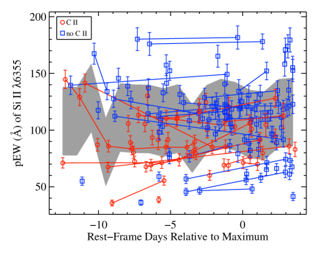
Figure 10: The temporal evolution of the Si ii $\lambda$6355 pEW for SNe Ia with C (red circles), without C (blue squares), and the 1$\sigma$ region around the average velocity as determined by the entire BSNIP sample (grey area). Objects with multiple velocity measurements are connected with a solid line.

As with the C ii velocities, no significant correlations were found between C ii pEW and light-curve width (parametrised by $\Delta m_{15}(B)$ or SALT2 $x_{1}$) or SN colour (parametrised by $\left(B-V\right)_{\rm max}$ or SALT2 $c$). Furthermore, no correlations were seen between pEW and synthetic photometric colours as derived from the spectra themselves (Section 4.3). Various spectroscopic luminosity and colour indicators (which are defined and discussed at length in BSNIP II and BSNIP III) were also found to be uncorrelated with C ii pEW. Moreover, no relationship was found between the pEW and velocity of either C ii feature.

Objects with and without C have similar O i triplet pEWs and both samples are similar to the O i triplet pEW distribution of the full BSNIP sample. The pEWs of most other spectral features seen in near-maximum spectra of SNe Ia showed no significant correlation with C ii pEW, except for the so-called Mg ii complex (with a correlation coefficient of $-0.73$). Figure 11 shows the 10 objects which have measured pEW values for both C ii $\lambda$6580 and the Mg ii complex. The solid line is the best linear fit to the data and the dotted lines are the root-mean square error. The plot symbols are the same as in Figure 7. If the two pEWs are measured in more than one spectrum of a given object, we only plot the spectrum that is closest to maximum brightness (i.e., the oldest) in Figure 11.

Figure 11: The pEW of the C ii $\lambda$6580 feature versus the pEW of the Mg ii complex. The data are highly correlated with a correlation coefficient of $-0.73$. The solid line is the best linear fit to the data and the dotted lines are the root-mean square error. The plot symbols are the same as in Figure 7.

The Mg ii complex was defined in BSNIP II and consists of a blend of many IGE spectral lines which encompasses a broad, complex absorption feature at 4100–4500 Å. In BSNIP III it was shown that both the pEWs of the Mg ii and Fe ii (another broad complex of IGE features at 4500–5200 Å) complexes were relatively good proxies for SALT2 colour ($c$, Guy et al., 2007), with increased pEW implying a redder colour. While the Fe ii complex is not very well correlated with pEW of C ii $\lambda$6580 (correlation coefficient of $-0.32$), the strong anti-correlation between the pEW of the Mg ii complex and the pEW of C ii indicates that increased pEW of C ii implies a bluer colour.

It has already been shown in this work that C-positive SNe Ia tend to have bluer colours than objects without C (Section 4.3). In light of the relationship between the pEWs of C ii and the Mg ii complex, perhaps this relationship with colour extends further than a simple binary splitting of objects with C versus those without C. It seems possible that the strength of the C feature is directly related to the colour of the SN. Objects where no C is detectable have the reddest colours, while objects with some C (i.e., low pEWs) have moderate colours, and finally objects with the most C (i.e., high pEWs) have the bluest colours. Unfortunately, as mentioned above, the pEW of the C ii $\lambda$6580 feature is not significantly correlated with any direct measure of the SN colour (via light curves or synthetic photometry from the spectra). The fact that the C ii pEW appears well correlated with two pEW-based spectral indicators of colour is intriguing, though, and should most definitely be investigated further in future studies.

5 Conclusions

In this work we have searched for signatures of unburned C from the progenitor WD using a subset of the BSNIP spectroscopic sample. We classify 188 spectra of 144 SNe Ia with ages $\la$3.6 d after maximum brightness as either showing definite C ii absorption (‘A’), possibly showing evidence for C (‘F’), definitely not showing C (‘N’), or inconclusive (‘?’). The spectrum-synthesis code SYNOW was used to accurately classify all spectra that showed possible evidence for C. The primary evidence for C is a distinct absorption line associated with C ii $\lambda$6580, though absorption from C ii $\lambda$7234 is also sometimes detected.

We find that $\sim\!\!$ 11 per cent of the SNe studied show definite C absorption features, while a total of $\sim\!\!$ 25 per cent show at least some evidence for C in their spectra, consistent with previous work (Parrent et al., 2011; Thomas et al., 2011; Folatelli et al., 2012). The detection rate of C decreases with time, though C can sometimes be seen at all ages younger than $\sim\!\!$ 4 d past maximum brightness. Near 4 d before maximum brightness, there is a 50 per cent probability of detecting C, according to the BSNIP data. If one obtains a spectrum at $t\la-5$ d, then there is a better than 30 per cent chance of detecting a distinct absorption feature from C ii.

Nearly all objects that show C are spectroscopically normal (as defined by various classification schemes), while SNe Ia without C detections are from all spectroscopic subtypes. The velocity gradients of objects with and without C have a similar average and range, and C detections and velocity gradients do not seem to be related in any way. However, we again point out that the BSNIP dataset is not well suited to velocity-gradient measurements. The light curves of SNe Ia with and without C also appear to have the same distribution. On the other hand, confirming previous work (Thomas et al., 2011; Folatelli et al., 2012), objects with C tend to have bluer optical colours than those without, and some (but not all) also have strong NUV excesses. This is shown with the BSNIP data using a variety of optical colour measurements.

The typical expansion velocity of the C ii $\lambda$6580 feature is 12,000–13,000 km s^-1, which is somewhat faster than the usual velocity measured for the C ii $\lambda$7234 feature (and we are the first to carefully study the velocity of this feature). The Si ii $\lambda$6355 velocities, measured in BSNIP II, tend to be lower than average for C-positive objects, while SNe Ia without C have a wide range of Si ii velocities. The ratio of the C ii $\lambda$6580 to Si ii $\lambda$6355 velocities is remarkably constant with time and among different objects, with a median value of $\sim\!\!$ 1.05 (consistent with what was reported by Parrent et al., 2011).

The pEWs of the C ii $\lambda$6580 and C ii $\lambda$7234 features are found mostly to decrease with time, though there is a significant increase between $\sim\!\!$ 13 and 11 d before maximum light. This is consistent with the predictions made by Folatelli et al. (2012) from spectral models based on those presented by Tanaka et al. (2011). The range of pEWs measured from the BSNIP data is consistent with earlier work and implies a range of C mass in SN Ia ejecta of $2\times 10^{-3}$ – $3\times 10^{-2}$ M_⊙ (Folatelli et al., 2012). C-positive objects tend to have slightly lower than average Si ii $\lambda$6355 pEWs, but at a relatively low significance. The pEW of the Mg ii complex is found to be strongly anti-correlated with the pEW of C ii $\lambda$6580, implying that bluer objects should have larger C ii pEWs. This is consistent withour finding that objects with obvious C tend to have bluer optical colours than those without. However, we find no strong correlation when comparing the pEW of C ii to direct measures of SN colour.

Even though this is the largest set of SNe Ia for which C has ever been searched, there are still only a handful of strong C detections and measurements of C absorption features. Other studies using independent datasets (Thomas et al., 2011; Folatelli et al., 2012) and literature searches (Parrent et al., 2011) have also been conducted, and we confirm most of their findings at higher significance. Still, many more moderate-to-high S/N SN Ia spectra at early epochs are needed to better investigate C and further probe WD progenitor models and SN Ia explosion mechanisms. New, large-scale transient searches such as Pan-STARRS (Kaiser et al., 2002) and the Palomar Transient Factory (PTF; Rau et al., 2009; Law et al., 2009) will be critical to moving this topic forward as they find progressively more young SNe of all types. One success story already is SN 2011fe (PTF11kly), discovered only 11 hr after explosion by PTF in M101, the Pinwheel Galaxy (Nugent et al., 2011; Li et al., 2011a). The search for and measurement of C in the many spectra of SN 2011fe obtained at extremely early epochs will further our quest to better understand SNe Ia.

References

- Amanullah et al. (2010) Amanullah R., et al., 2010, ApJ, 716, 712
- Astier et al. (2006) Astier P., et al., 2006, A&A, 447, 31
- Benetti et al. (2005) Benetti S., et al., 2005, ApJ, 623, 1011
- Bessell (1990) Bessell M. S., 1990, PASP, 102, 1181
- Blondin & Tonry (2007) Blondin S., Tonry J. L., 2007, ApJ, 666, 1024
- Branch et al. (2009) Branch D., Dang L. C., Baron E., 2009, PASP, 121, 238
- Branch et al. (2006) Branch D., Dang L. C., Hall N., Ketchum W., Melakayil M., Parrent J., Troxel M. A., Casebeer D., Jeffery D. J., Baron E., 2006, PASP, 118, 560
- Branch et al. (2003) Branch D., et al., 2003, AJ, 126, 1489
- Cardelli et al. (1989) Cardelli J. A., Clayton G. C., Mathis J. S., 1989, ApJ, 345, 245
- Chornock et al. (2006) Chornock R., Filippenko A. V., Branch D., Foley R. J., Jha S., Li W., 2006, PASP, 118, 722
- Colgate & McKee (1969) Colgate S. A., McKee C., 1969, ApJ, 157, 623
- Filippenko (1997) Filippenko A. V., 1997, ARA&A, 35, 309
- Filippenko et al. (1992a) Filippenko A. V., et al., 1992a, ApJ, 384, L15
- Filippenko et al. (1992b) Filippenko A. V., et al., 1992b, AJ, 104, 1543
- Fisher et al. (1997) Fisher A., Branch D., Nugent P., Baron E., 1997, ApJ, 481, L89
- Folatelli et al. (2012) Folatelli G., et al., 2012, ApJ, 745, 74
- Foley et al. (2009) Foley R. J., et al., 2009, AJ, 138, 376
- Gamezo et al. (2003) Gamezo V. N., Khokhlov A. M., Oran E. S., Chtchelkanova A. Y., Rosenberg R. O., 2003, Science, 299, 77
- Ganeshalingam et al. (2010) Ganeshalingam M., et al., 2010, ApJS, 190, 418
- Garavini et al. (2004) Garavini G., et al., 2004, AJ, 128, 387
- Garavini et al. (2005) Garavini G., et al., 2005, AJ, 130, 2278
- Garavini et al. (2007) Garavini G., et al., 2007, A&A, 470, 411
- Gehrels et al. (2004) Gehrels N., et al., 2004, ApJ, 611, 1005
- Guy et al. (2007) Guy J., et al., 2007, A&A, 466, 11
- Hachinger et al. (2006) Hachinger S., Mazzali P. A., Benetti S., 2006, MNRAS, 370, 299
- Hatano et al. (1999) Hatano K., Branch D., Fisher A., Millard J., Baron E., 1999, ApJS, 121, 233
- Hicken et al. (2009) Hicken M., Wood-Vasey W. M., Blondin S., Challis P., Jha S., Kelly P. L., Rest A., Kirshner R. P., 2009, ApJ, 700, 1097
- Hillebrandt & Niemeyer (2000) Hillebrandt W., Niemeyer J. C., 2000, ARA&A, 38, 191
- Höflich et al. (2002) Höflich P., Gerardy C. L., Fesen R. A., Sakai S., 2002, ApJ, 568, 791
- Howell et al. (2006) Howell D. A., et al., 2006, Nature, 443, 308
- Hoyle & Fowler (1960) Hoyle F., Fowler W. A., 1960, ApJ, 132, 565
- Jha et al. (2006) Jha S., Branch D., Chornock R., Foley R. J., Li W., Swift B. J., Casebeer D., Filippenko A. V., 2006, AJ, 132, 189
- Jha et al. (2007) Jha S., Riess A. G., Kirshner R. P., 2007, ApJ, 659, 122
- Kaiser et al. (2002) Kaiser N., et al., 2002, in Tyson J. A., Wolff S., eds, Proceedings of the Society of Photo-Optical Instrumentation Engineers (SPIE) Conference. Vol. 4836. p. 154
- Kasen et al. (2009) Kasen D., Röpke F. K., Woosley S. E., 2009, Nature, 460, 869
- Kessler et al. (2009) Kessler R., et al., 2009, ApJS, 185, 32
- Law et al. (2009) Law N. M., et al., 2009, PASP, 121, 1395
- Leibundgut et al. (1993) Leibundgut B., et al., 1993, AJ, 105, 301
- Li et al. (2001) Li W., et al., 2001, PASP, 113, 1178
- Li et al. (2003) Li W., et al., 2003, PASP, 115, 453
- Li et al. (2011a) Li W., et al., 2011a, Nature, 480, 348
- Li et al. (2011b) Li W., et al., 2011b, MNRAS, 412, 1441
- Li et al. (2001) Li W., Filippenko A. V., Treffers R. R., Riess A. G., Hu J., Qiu Y., 2001, ApJ, 546, 734
- Lucy (1999) Lucy L. B., 1999, A&A, 345, 211
- Marion et al. (2006) Marion G. H., Höflich P., Wheeler J. C., Robinson E. L., Gerardy C. L., Vacca W. D., 2006, ApJ, 645, 1392
- Mazzali (2000) Mazzali P. A., 2000, A&A, 363, 705
- Mazzali (2001) Mazzali P. A., 2001, MNRAS, 321, 341
- Mazzali & Lucy (1993) Mazzali P. A., Lucy L. B., 1993, A&A, 279, 447
- Miller & Stone (1993) Miller J. S., Stone R. P. S., 1993, Lick Obs. Tech. Rep. 66. Santa Cruz: Lick Obs.
- Milne & Brown (2012) Milne P. A., Brown P. J., 2012, Extreme and Variable High Energy Sky 2011, submitted (arXiv:1201.1279)
- Milne et al. (2010) Milne P. A., et al., 2010, ApJ, 721, 1627
- Nomoto et al. (1984) Nomoto K., Thielemann F.-K., Yokoi K., 1984, ApJ, 286, 644
- Nugent et al. (1995) Nugent P., Phillips M., Baron E., Branch D., Hauschildt P., 1995, ApJ, 455, L147
- Nugent et al. (2011) Nugent P. E., et al., 2011, Nature, 480, 344
- O’Donnell (1994) O’Donnell J. E., 1994, ApJ, 422, 158
- Parrent et al. (2011) Parrent J. T., Thomas R. C., Fesen R. A., Marion G. H., Challis P., Garnavich P. M., Milisavljevic D., Vinkò J., Wheeler J. C., 2011, ApJ, 732, 30
- Patat et al. (1996) Patat F., Benetti S., Cappellaro E., Danziger I. J., Della Valle M., Mazzali P. A., Turatto M., 1996, MNRAS, 278, 111
- Perlmutter et al. (1999) Perlmutter S., et al., 1999, ApJ, 517, 565
- Phillips (1993) Phillips M. M., 1993, ApJ, 413, L105
- Phillips et al. (2007) Phillips M. M., et al., 2007, PASP, 119, 360
- Phillips et al. (1992) Phillips M. M., Wells L. A., Suntzeff N. B., Hamuy M., Leibundgut B., Kirshner R. P., Foltz C. B., 1992, AJ, 103, 1632
- Rau et al. (2009) Rau A., et al., 2009, PASP, 121, 1334
- Riess et al. (1998) Riess A. G., et al., 1998, AJ, 116, 1009
- Riess et al. (2007) Riess A. G., et al., 2007, ApJ, 659, 98
- Roming et al. (2005) Roming P. W. A., et al., 2005, Space Sci. Rev., 120, 95
- Röpke et al. (2007) Röpke F. K., Hillebrandt W., Schmidt W., Niemeyer J. C., Blinnikov S. I., Mazzali P. A., 2007, ApJ, 668, 1132
- Savitzky & Golay (1964) Savitzky A., Golay M. J. E., 1964, Analytical Chemistry, 36, 1627
- Scalzo et al. (2010) Scalzo R. A., et al., 2010, ApJ, 713, 1073
- Silverman et al. (2012) Silverman J. M., et al., 2012, MNRAS, submitted (arXiv:1202.2128)
- Silverman et al. (2011) Silverman J. M., Ganeshalingam M., Li W., Filippenko A. V., Miller A. A., Poznanski D., 2011, MNRAS, 410, 585
- Silverman et al. (2012) Silverman J. M., Kong J. J., Filippenko A. V., 2012, MNRAS, submitted (arXiv:1202.2129)
- Stanishev et al. (2007) Stanishev V., et al., 2007, in di Salvo T., Israel G. L., Piersant L., Burderi L., Matt G., Tornambe A., T. M. M., eds, The Multicolored Landscape of Compact Objects and Their Explosive Origins. Vol. 924. pp 336–341
- Strolger et al. (2002) Strolger L., et al., 2002, AJ, 124, 2905
- Suzuki et al. (2012) Suzuki N., et al., 2012, ApJ, 746, 85
- Tanaka et al. (2008) Tanaka M., et al., 2008, ApJ, 677, 448
- Tanaka et al. (2011) Tanaka M., Mazzali P. A., Stanishev V., Maurer I., Kerzendorf W. E., Nomoto K., 2011, MNRAS, 410, 1725
- Taubenberger et al. (2011) Taubenberger S., et al., 2011, MNRAS, 412, 2735
- Thomas et al. (2007) Thomas R. C., et al., 2007, ApJ, 654, L53
- Thomas et al. (2011) Thomas R. C., et al., 2011, ApJ, 743, 27
- Thomas et al. (2011) Thomas R. C., Nugent P. E., Meza J. C., 2011, PASP, 123, 237
- Valenti et al. (2009) Valenti S., et al., 2009, Nature, 459, 674
- Wang et al. (2009) Wang X., et al., 2009, ApJ, 699, L139
- Wood-Vasey et al. (2007) Wood-Vasey W. M., et al., 2007, ApJ, 666, 694
- Yamanaka et al. (2009) Yamanaka M., et al., 2009, ApJ, 707, L118