Measuring X-ray variability in faint/sparsely-sampled AGN

Abstract

We study the statistical properties of the Normalized Excess Variance of variability process characterized by a “red-noise” power spectral density (PSD), as the case of Active Galactic Nuclei (AGN). We perform Monte Carlo simulations of lightcurves, assuming both a continuous and a sparse sampling pattern and various signal-to-noise (S/N) ratios. We show that the normalized excess variance is a biased estimate of the variance even in the case of continuously sampled lightcurves. The bias depends on the PSD slope and on the sampling pattern, but not on the S/N ratio. We provide a simple formula to account for the bias, which yields unbiased estimates with an accuracy better than $15$%. We show that the normalized excess variance estimates based on single lightcurves (especially for sparse sampling and S/N $<$ 3) are highly uncertain (even if corrected for bias) and we propose instead the use of an “ensemble estimate”, based on multiple lightcurves of the same object, or on the use of lightcurves of many objects. These estimates have symmetric distributions, known errors, and can also be corrected for biases.We use our results to estimate the ability to measure the intrinsic source variability in current data, and show that they could also be useful in the planning of the observing strategy of future surveys such as those provided by X-ray missions studying distant and/or faint AGN populations and, more in general, in the estimation of the variability amplitude of sources that will result from future surveys such as Pan-STARRS, and LSST.

1. Introduction

Active Galactic Nuclei (AGN) are characterized by large amplitude and rapid variability, especially in the X-ray band, which is probably originating in the inner regions of the accretion disk and the hot corona in Seyfert AGNs. One of the most common tools for examining AGN variability is the Power Spectral Density Function (PSD). Early attempts to measure the AGN X-ray PSDs showed that they have a power-law like shape with a slope of $\sim-1.5$ (Green et al., 1993; Lawrence & Papadakis, 1993), although PSDs as steep as $-3$ have been observed in X-ray light curves of radio-loud sources (Kataoka et al., 2001) or in optical AGN lightcurves (Mushotzky et al., 2011). This result is indicative of a scale-invariant red-noise process, on timescales ranging from a few hours to years, with no evidence of periodicities (with the possible exception of RE J1034+396 reported by Gierliński et al., 2008).

In recent years it has become increasingly clear that there exists at least one characteristic timescale in the AGN X-ray PSDs. This timescale reveals itself in the form of ”frequency breaks” ($\nu_{\rm br}$) in the PSD, where the slope changes from a value of $\sim-1$ below the ”break”, to $\sim-2$ at frequencies higher than $\nu_{\rm br}$ (see e.g. 2002; Markowitz et al. 2003). These time scales may be linked to the characteristic disk time scales like the dynamical, thermal or viscous timescale, and appear to correlate with the black hole (BH) mass and accretion rate (McHardy et al., 2006; Koerding et al., 2007; González-Martín & Vaughan, 2012). Thus variability measurements represent a tool to investigate both the physics of the accretion process, as well as the fundamental parameters ($M_{\rm BH}$, $\dot{m}$) of the active nucleus.

So far, our knowledge of the X-ray variability properties of AGN is mainly based on the study of a few nearby, X-ray bright objects, which have been monitored extensively with Rossi X-ray Timing Explorer (RXTE) over many years, and for which there also exist day-long, high signal-to-noise (S/N) XMM-Newton lightcurves. However several authors have also studied the ensemble variability properties of AGN populations making use of different statistics (e.g., O’Neil et al., 2005; Zhou et al., 2010; Vagnetti et al., 2011; Zhang et al., 2011; Ponti et al., 2012). The most commonly adopted statistics in these studies for the measure of the variability amplitude is the so called normalized excess variance, $\sigma^{2}_{\rm NXV}$ (Nandra et al., 1997; Turner et al., 1999; Edelson et al., 2002).

One of the main results of these investigations is that $\sigma^{2}_{\rm NXV}$ anti-correlates with the mass of the central compact object (e.g., Papadakis et al., 2004; Nikolajuk, Papadakis & Czerny, 2004; O’Neil et al., 2005; Zhou et al., 2010). In fact, it has been suggested that $\sigma^{2}_{\rm NXV}$ can be used to measure the mass of the central black hole (BH) in AGN (e.g., Nikolajuk, Papadakis & Czerny, 2004; Gierlinski, Nikolajuk & Czerny, 2008; Ponti et al., 2012) and in other objects like the Ultraluminous X-ray sources Gonzalez-Martini et al. (2011). Furthermore, recent deep multi-cycle surveys (e.g. 2003, 2008; Comastri et al. 2011; Xue et al. 2011; also see Brandt & Hasinger 2005 and references therein), have been accumulating observations of intermediate and high ($z>0.5$) redshift AGN, thus offering the opportunity to explore AGN variability at high redshift as well. However, due to the sparse (i.e. uneven and with large gaps) sampling, and the low flux of most AGN detected in these surveys, it is not possible to use PSD techniques to study the variability properties of these objects. Also in these cases $\sigma^{2}_{\rm NXV}$ has been used to parametrize the variability properties of the high redshift AGN (, 2000; Paolillo et al., 2004; Papadakis et al., 2008).

Despite the relative importance of the normalized excess variance as a tool to measure variability amplitude in AGN, as well as a tool to measure BH mass in these, and perhaps other accreting objects as well, there have not been many studies to investigate its statistical properties. A systematic discussion of the statistical properties of $\sigma^{2}_{\rm NXV}$ and its performance in the case of red noise PSDs of various slopes and different signal-to-noise (S/N) ratios, can be found in Vaughan et al. (2003). This work demonstrated that $\sigma^{2}_{\rm NXV}$ extrapolations from any single realization can be misleading due to the stochastic nature of any red-noise lightcurve, and quantifies the expected uncertainties in order to, e.g. compare the same lightcurve in different energy bands. However, even these authors have not considered explicitly the question whether $\sigma^{2}_{\rm NXV}$ is an unbiased estimate of the intrinsic source variance or not, and have considered the case of continuously sampled data only, such as those provided by long XMM observations of nearby AGNs. Instead, in serendipitous datasets, as well as in deep multi-cycle surveys, the effects of sparse sampling must be taken taken into account when investigating the statistical properties of the excess variance.

To some extent, this work is thus an extension of the work done by Vaughan et al (2003). Our goal is to investigate the statistical properties of the excess variance (i.e. scatter, and the mean) in the case of both evenly and sparsely sampled light curves, whose PSD has a “red noise” shape. We pay particular attention to the case of highly uneven patterns, like those in light curves which result from current multi-epoch surveys. This pattern is characterized by extreme sparsity due to the observing strategy and orbital visibility of the targets. We consider various PSD slopes, sampling patterns, as well as S/N ratios, and we perform detailed Monte-Carlo numerical experiments to investigate the statistical properties (mean, standard deviation and skewness) of the excess variance in each case. The results are used to derive some simple recipes to acquire excess variance measurements that will be unbiased estimates of the intrinsic variance (to a large extent), and will follow a Gaussian distribution with known errors, thus rendering them eligible to compare with theoretical predictions using the frequently used $\chi^{2}$ minimization techniques.

2. Normalized Excess Variance

The so called normalized excess variance, $\sigma^{2}_{\rm NXV}$, is defined as (Nandra et al., 1997):

$$\sigma^{2}_{\rm NXV}=\frac{1}{N\overline{x}^{2}}\sum_{i=1}^{N}\,[(x_{i}-\overline{x})^{2}-\sigma_{\rm err,\textit{i}}^{2}],$$ (1)

where $x_{i}$ and $\sigma_{\rm err,\textit{i}}$ are the count rate and its error in i-th bin, $\overline{x}$ is the mean count rate , and $N$ is the number of bins used to estimate $\sigma^{2}_{\rm NXV}$. With this normalization we are able to compare excess variance estimates derived from different segments of a particular lightcurve or from lightcurves of different sources. Nandra et al. (1997) also provided an error estimate on $\sigma^{2}_{\rm NXV}$, which is based on the variance of the quantity $(x_{i}-\overline{x})^{2}-\sigma_{\rm err,\textit{i}}^{2}$, i.e.

$$\Delta\sigma^{2}_{\rm NXV} = S_{D}/[\overline{x}^{2}(N)^{1/2}],$$ (2)

$$S_{D} = \frac{1}{N-1}\sum_{i=1}^{N}\,\{[(x_{i}-\overline{x})^{2}-\sigma_{\rm err,\textit{i}}^{2}]-\sigma^{2}_{\rm NXV}\overline{x}^{2}\}^{2}.$$

Almaini et al (2000) proposed an alternative normalized excess variance estimate, $\sigma^{2}_{\rm ML}$, which they argued will perform better in the case when the errors on the lightcurve points are not identical and they are not normally distributed. There is no analytical equation for this estimate, as it is based on a maximum-likelihood approach, and the estimate has to be determined numerically for a given lightcurve (see their § 3.1 for details).

If $\mu$ and $\sigma^{2}$ are the intrinsic mean and variance of a lightcurve, $\sigma^{2}_{\rm NXV}$ and $\sigma^{2}_{\rm ML}$ are though to be an estimate of intrinsic normalized source variance, i.e. $\sigma^{2}_{\rm norm}=\sigma^{2}/\mu^{2}$. However, this assumption has never been investigated thoroughly in the case when the light curve in question is a realization of process which has an intrinsic ”red-noise” power spectrum. In this case, there are a few reasons to believe that this assumption may not hold. This can be understood if one considers the fact that the intrinsic power spectral density function, $PSD(\nu)$, of a time series is defined in such a way so that:

$$\sigma^{2}=\int_{0}^{\infty}PSD(\nu)d\nu.$$ (3)

As we mentioned above, based on the detailed studies of $\sim$15-20 nearby AGN, these sources (as well as the Galactic X-ray accreting objects) exhibit a power-law X-ray PSD at high frequencies of the form of $PSD(\nu)\propto\nu^{-\beta}$, with $\beta\sim 2$. There exists a ”break frequency”, $\nu_{\rm br}$, where the PSD slope flattens to a slope of $\beta\sim 1$ at lower frequencies. This ”break frequency” depends on the BH mass of the system, and the respective ”break time scale” (i.e. $1/\nu_{\rm br}$) increases proportionally with the BH mass (e.g., McHardy et al., 2006; González-Martín & Vaughan, 2012). It is of the order of $\sim$ few tens of minutes for BH masses of $\sim 10^{6}$ M_⊙, and increases to $\sim$ a day or so for BH masses $\sim 10^{8}$ M_⊙. A second break to a slope of $\sim 0$ is expected at even lower frequencies, for the integral in Eq. 3 to converge, as expected for a stationary process. Such breaks are routinely observed in Galactic X-ray Black Hole binary candidates when in the so called ”low/hard” state. It has also been observed in one AGN (namely Ark 564, Papadakis et al. 2002; McHardy et al. 2007). However, in all other cases, the AGN PSDs exhibit a power-law shape with a slope of $\beta\sim 1$ at all sampled frequencies, which can be as low as $1/(10-20)$ years^-1 in the case of a few AGN which were regularly monitored by RXTE for more than a decade (e.g. NGC 4051, McHardy et al. 2004; MCG–6-30-15, McHardy et al. 2005).

If $\sigma^{2}_{\rm NXV}$ or $\sigma^{2}_{\rm ML}$ are computed using a lightcurve whose duration, $T_{\rm max}$, is shorter than the time scale at which the transition from the slope of $-1$ to zero appears in the intrinsic PSD, then: a) $\overline{x}$ may not be an accurate estimate of $\mu$, so one has to investigate what are the effects of using $\overline{x}$ (as opposed to $\mu$) in the definition of $\sigma^{2}_{\rm NXV}$ in Eq. 1, and b) $\sigma^{2}_{\rm NXV}$ or $\sigma^{2}_{\rm ML}$ may underestimate $\sigma^{2}_{\rm norm}$, as there will be intrinsic variations on time scales longer than $T_{\rm max}$, which cannot be fully sampled in the given light curve.

For these reasons Ponti et al. (2012) as well as most of the aforementioned papers by Nikolajuk et al., Gonzalez et al., O’Neill et al. and Papadakis et al. (2008) have assumed that $\sigma^{2}_{\rm NXV}$ is a measure of the intrinsic ”band” normalized variance, defined as,

$$\sigma^{2}_{\rm band,norm}=\left[\int_{1/T_{\rm max}}^{1/T_{\rm min}}PSD(\nu)d\nu\right]/\mu^{2}.$$ (4)

where $\mu$ and $PSD(\nu)$ are the intrinsic mean and PSD of the time series.

The ”band” normalized variance measures the contribution to the total variance (normalized to the mean squared) of all the variability components with frequencies higher than 1/$T_{\rm max}$ (i.e. the longest, fully sampled frequency) and lower than 1/$T_{\rm min}$ (i.e. the highest sample frequency since $T_{\rm min}=2\times\Delta t$, where $\Delta t$ is the the bin size of the observed light curve).

However, even the assumption that $\sigma^{2}_{\rm NXV}$ or $\sigma^{2}_{\rm ML}$ are estimates of the $\sigma^{2}_{\rm band,norm}$ has not been tested in practice, and there are reasons to believe that it may not be entirely accurate in the case of ”red-noise” PSDs. The first reason is that, although variations on time scales longer than $T_{\rm max}$ are not fully sampled in a lightcurve with a length of $T_{\rm max}$, they can still contribute to its variance (this is the so-called ”red-noise leakage” problem). As a result, $\sigma^{2}_{\rm NXV}$ may overestimate $\sigma^{2}_{\rm band,norm}$. Secondly, in the case of sparsely sampled lightcurves, not all variability components will be sampled with the same ”accuracy”, while the ability to recover intrinsic $\sigma^{2}_{\rm band,norm}$ for faint sources may be undermined by the relatively stronger experimental noise level. Finally, in reality, the intrinsic PSD should continue with a power-law shape to frequencies higher than $1/T_{\rm min}$. Consequently, the observed normalized excess variance may again overestimate the intrinsic “band” normalised variance, as defined in equation (4), due to aliasing effects. However, since the observed light curves are not sampled every $\Delta t$, but they are binned over intervals of size equal to $\Delta t$, any variations at frequencies higher than $1/(2\Delta t)$ are smeared out, and we do not expect the estimated normalized excess variance to be significantly affected by the intrinsic power at these high frequencies.

In the following sections we perform detailed Monte-Carlo simulations with the intent to verify if $\sigma^{2}_{\rm NXV}$ and $\sigma^{2}_{\rm ML}$ can be considered as accurate estimates of $\sigma^{2}_{\rm band,norm}$ in the case of red-noise PSDs, and we further explore their statistical properties in the case of sparse sampling and sources with low S/N ratio lightcurves.

3. Monte Carlo Simulations: The algorithm and the relevant statistical parameters

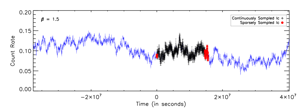
Figure 1.— Simulated lightcurve (continuous blue line) in the case of a PSD with $\beta=1.5$. Black crosses with errorbars show the ”continuously sampled lightcurve” while the red dots indicate the ”sparsely sampled lightcurve”.

We performed Monte Carlo simulations by using the code of Timmer & Koenig (1995). This code is appropriate for the generation of Gaussian light curves with a given PSD. It is not clear whether Gaussianity applies to the AGN light curves (in any spectral band), and in fact, it is almost certain that it does not apply to the light curves of blazars. However, exploring the effects of non-Gaussianity to our results are beyond the scope of our paper. We also assume an AGN PSDs of light curves that are Gaussian and that remain only weakly non-stationary (following the definition as in Section 4.1 of Vaughan et al. 2003) on time scales of decades and shorter. As for Gaussianity, exploring the effects of non-stationarity is beyond the scope of this work. We modified the original code that generates red-noise data with a power law PSD, in order to reproduce the real data extraction process including filtering and background subtraction. We first created an evenly sampled AGN lightcurve with the above algorithm, following the appropriate PSD (see below). Then we added to the AGN count rate, in each time bin, the contribution from the expected (instrumental and cosmic) background along the line-of-sight to the source, randomly adding Poisson fluctuations to both terms. A second background estimate is also generated (including again Poisson fluctuations), simulating the one measured in a nearby region in real data, and then subtracted from the total counts in each bin, as done for real sources.

As a starting point, we simulated red-noise lightcurves with intrinsic count rate of $\mu_{\rm full}=0.099$ cnt s^-1 and variance, $\sigma^{2}_{\rm full}$, such that $\sigma^{2}_{\rm full,norm}=\sigma^{2}_{\rm full}/\mu_{\rm full}^{2}=0.042$ (see Table 1). These are equal to the mean and normalized variance (after correcting for the Poisson noise) of the brightest AGN observed by XMM-Newton in the CDFS (source id 68 from Giacconi et al., 2002) at $z\sim 0.54$. The source has an identical soft 0.5-2 keV and hard 2-8 keV flux of $\sim 5\times 10^{-14}$ erg cm^-2 s^-1, i.e. we expect 10-20 of these sources per square degree, according to, e.g. Hasinger et al. (1993); Luo et al. (2008). Compared to other bright AGN in the field, this source has the advantage of being fairly isolated and thus its flux and variability can be robustly estimated. We point out that in our simulations we assume an PSD with the appropriate normalization in order to yield the required intrinsic variance and flux, and we do not renormalize the lightcurves a-posteriori after creating them, since the latter method would produce lightcurves which do not span the full range of mean fluxes and variances.

We considered the sampling pattern of the first 1Ms XMM-Newton observations of the Chandra Deep Field South (CDFS, Comastri et al., 2011). XMM-Newton observed CDFS once in July 2001 with an effective exposure, after filtering high background periods, of $\sim 80$ ks and then, six times in January 2002 for additional $370$ ks. The time interval between the start of the first observation and the end of the last one (i.e. the longest time scale sampled by the 1Ms XMM-CDFS lightcurves) is $T_{\rm max}=1.56\times 10^{7}$sec, i.e. about 6 months. The actual XMM-CDFS observations lasted for $\sim 4.5\times 10^{5}$ sec ($\sim$ 5 days) during this period of 6 months. This type of observing pattern is a ”worst-case” scenario (in terms of sparse sampling): the total exposure time is only $\sim 3$% of the observing period, and the data are collected in two blocks at the start and at the end of the observing period. This type of observing pattern is driven primarily by the typical scheduling requirements of deep multi-cycle campaigns, and thus represents a recurring, although undesirable, observing scheme . We nevertheless adopted it in order to study the effects of sparse sampling in an ”extreme” case, before discussing, in the next sections, more favourable sampling patterns.

We considered lightcurves whose PSD has a power-law shape of the form: $PSD(\nu)\propto\nu^{-\beta}$, where $\beta=1,1.5,2,2.5$ and 3. In the figures throughout the paper we present the results for the simulations with $\beta=1.5$, but we always discuss the results in the other cases as well. In order to account for the effect of red noise leak, which transfers power from low (undersampled) to high frequencies, we generated lightcurves which are 5 times longer than the longest timescale sampled by the data we considered. We verified in the case of $\beta=3$ that extending the simulated lightcurves by a factor of 10 does not significantly changes our results, while increasing considerably the processing time. Hence, we are confident that our simulations take into account properly the ”red-noise” leak effects, even in the case of the PSDs with slopes steeper than 2.

For each $\beta$, we produced 5000 simulated lightcurves with a length equal to $T_{\rm max,full}=5\times T_{\rm max}$. We assumed a bin size of $\Delta t=10$ ks (so that $T_{\rm min}$ in equation (4) is equal to 20 ksec). This is typical for relatively faint sources, where a large bin size is required to increase the S/N ratio, hence decreasing the contribution of the experimental Poisson noise in the observed variations. As a result, our original lightcurves had 7800 points in them. We randomly chose a lightcurve segment with a length equal to $T_{\rm max}$, and then, we chose these points from this segment which reproduce the actual observing pattern of the 1Ms XMM-CDFS observations.

Figure 1 shows an example of the simulated lightcurve in the case of $\beta=1.5$ PSD. The blue continuous line indicates the full lightcurve. Black crosses with error bars indicate the data points in the lightcurve segment of size $T_{\rm max}$ that we randomly chose (hereafter ”continuously sampled lightcurve”), while the red points indicate the actual XMM-CDFS observations, that were performed within this interval (hereafter ”sparsely sampled light curve”).

The blue dotted line in Figure 2 indicates the periodogram of the full lightcurve indicated with the blue points in Figure 1. The red solid line in the same figure indicates the input PSD, with a slope of $\beta=1.5$. The agreement between the periodogram of the full simulated lightcurve and the ”input” PSD is very good. The black solid line indicates the periodogram of the ”continuous” lightcurve segment (which is indicated with the black points in Figure 1). This is not significantly different than the intrinsic PSD either. This is probably due to the fact that red-noise aliasing effects are not extreme in the case of PSDs with slopes less than 2.

For each one of the 5000 simulated lightcurves (like the one shown in Figure 1) we computed the sample mean of the randomly chosen ”continuously” and ”sparsely” sampled lightcurves ($\overline{x}_{\rm cont}$ and $\overline{x}_{\rm sparse}$, respectively) and their normalized excess variance using Eq. 1 ($\sigma^{2}_{\rm NXV,cont}$ and $\sigma^{2}_{\rm NXV,sparse}$, respectively). We also computed the ML variance estimator as proposed by (2000) for the sparsely sampled lightcurves ($\sigma^{2}_{\rm ML,sparse}$). Using the 5000 values of $\sigma^{2}_{\rm NXV,cont}$, $\sigma^{2}_{\rm NXV,sparse}$  and $\sigma^{2}_{\rm ML,sparse}$, we constructed their sample distributions, and we computed their mean values (denoted with brackets, i.e. $\langle$ $\sigma^{2}_{\rm NXV,cont}$ $\rangle$, etc), standard deviation, and skewness.

Finally, for each PSD slope $\beta$, we also calculated $\sigma^{2}_{\rm band,norm}$ using Eq. (4). Since the same equation holds for $\sigma^{2}_{\rm full}$ as well (with $\nu_{\rm min,full}=1/T_{\rm max,full}$, and $\nu_{\rm max,full}=1/T_{\rm min}$), one can easily show that:

$$\sigma^{2}_{\rm band,norm}=\sigma^{2}_{\rm full,norm}\times\frac{(T_{\rm max}/T_{\rm min})^{\beta-1}-1}{(T_{\rm max,full}/T_{\rm min})^{\beta-1}-1},$$ (5)

in the case of PSDs with $\beta>1$, and:

$$\sigma^{2}_{\rm band,norm}=\sigma^{2}_{\rm full,norm}\times\frac{\ln(T_{\rm min}/T_{\rm max})}{\ln(T_{\rm min}/T_{\rm max,full})},$$ (6)

in the case of PSDs with $\beta=1$. The $\sigma^{2}_{\rm band,norm}$ values for the different PSD slopes are listed in Table 2. Note that, although $\sigma^{2}_{\rm full,norm}$, $T_{\rm max}$ and $T_{\rm min}$ are the same for all the simulations we performed, $\sigma^{2}_{\rm band,norm}$ decreases significantly with increasing $\beta$, as more power is stored in the low frequency components for steeper PSDs.

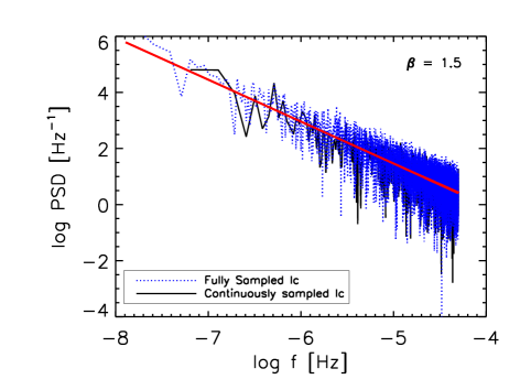
Figure 2.— Periodogram derived from the lightcurves shown in Figure 1. The blue dotted line corresponds to the periodogram of the full lightcurve (blue line in Figure 1), with the red line showing the input PSD. The black line corresponds to the periodogram of the continuously sampled lightcurve (black points in Figure 1).

Table 1Input parameters of the simulated AGN lightcurves

Power-law PSD index ($\beta$)	1,1.5,2,2.5,3
Number of simulations ($N$)	5000
$\mu_{\rm full}$	0.099 cnt s-1
Time resolution ($\Delta t$)	10 ks
$\sigma^{2}_{\rm full,norm}$	$0.042$
Background level	0.06 cnt s-1

4. The distribution of the normalized excess variance, in the case of red noise PSDs

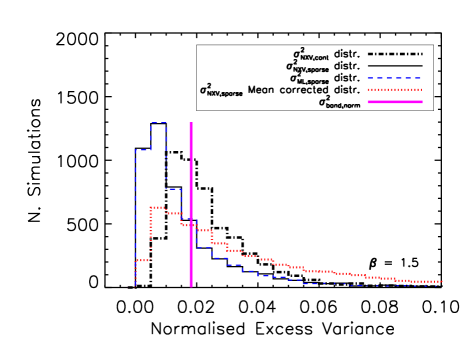
Figure 3.— The $\sigma^{2}_{\rm NXV,sparse}$, $\sigma^{2}_{\rm NXV,cont}$, and $\sigma^{2}_{\rm ML,sparse}$ distributions (black solid, black dot-dashed lines, and dashed blue lines, respectively), compared to $\sigma^{2}_{\rm band,norm}$ (vertical red solid line), for the $\beta=1.5$ PSD. The dotted red line indicates the $\sigma^{2}_{\rm NXV,sparse}$ distribution, when $\sigma^{2}_{\rm NXV}$ is computed using the intrinsic mean count rate $\mu_{\rm full}$ (see discussion in the text).

Table 2Statistical properties (mean/standard deviation/skewness), formal error and bias of the variance distributions

$\beta$	$\sigma^{2}_{\rm band,norm}$	$\sigma^{2}_{\rm NXV,cont}$	$\Delta\sigma^{2}_{\rm NXV}$	$\sigma^{2}_{\rm NXV,sparse}$	$\Delta\sigma^{2}_{\rm NXV}$	$\sigma^{2}_{\rm ML,sparse}$	$\sigma^{2}_{\rm NXV,sparse}$	$b_{\rm cont}$	$b_{\rm sparse}$
			Eq. 2		Eq. 2		Mean Corr.
1	0.034	0.037/0.01/1.35	0.001	0.029/0.017/3.35	0.006	0.029/0.017/3.29	0.042/0.026/2.44	0.92	1.19
1.5	0.018	0.025/0.016/2.55	0.0008	0.019/0.025/5.24	0.004	0.019/0.025/5.16	0.043/0.044/2.57	0.74	1.00
2	0.0084	0.016/0.016/3.42	0.0004	0.014/0.023/5.52	0.003	0.014/0.023/5.48	0.042/0.048/2.58	0.49	0.57
2.5	0.0037	0.012/0.015/3.81	0.0003	0.012/0.022/6.03	0.003	0.012/0.022/6.09	0.041/0.048/2.42	0.31	0.30
3	0.0017	0.010/0.013/4.11	0.0003	0.012/0.023/8.12	0.003	0.012/0.023/8.20	0.042/0.051/2.59	0.17	0.14

The black dot-dashed, black solid and blue dashed lines in Figure 3 indicate the $\sigma^{2}_{\rm NXV,cont}$, $\sigma^{2}_{\rm NXV,sparse}$, and $\sigma^{2}_{\rm ML,sparse}$ distributions, using the results from the set of the 5000 simulations for the case of the $\beta=1.5$ PSD. Although the errors on each lightcurve point are not identical (see §2), the $\sigma^{2}_{\rm ML,sparse}$ distribution does not differ significantly from the distribution of the $\sigma^{2}_{\rm NXV,sparse}$ values.

All distributions are broad and asymmetric. They are skewed, and show long tails towards values larger than $\sigma^{2}_{\rm band,norm}$ (which is indicated by the vertical solid line in the same plot). This is mainly due to the fact that the excess variance follows a $\chi^{2}_{N}$ distribution (see Vaughan et al. 2003). At the same time, a large number of normalized variance values are quite smaller than $\sigma^{2}_{\rm band,norm}$. This is particularly true with the $\sigma^{2}_{\rm NXV,sparse}$ and $\sigma^{2}_{\rm ML,sparse}$ distributions, because in many cases the data points in the sparsely sampled light curves are “clustered” close to their sample mean, hence resulting in sample variances smaller than the intrinsic value.

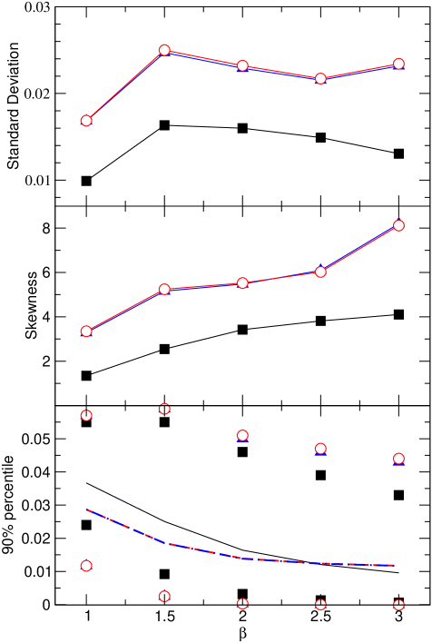
Figure 4.— Standard deviation, skewness and 90% percentiles of the $\sigma^{2}_{\rm NXV,cont}$, $\sigma^{2}_{\rm NXV,sparse}$ and $\sigma^{2}_{\rm ML,sparse}$ distributions (filled black squares, open red circles, and filled blue triangles, respectively) plotted as function of $\beta$. In the lower panel the black continuous, red dashed and blue dot-dashed lines represent the sample means as reported in Table 2.

The mean, standard deviation and skewness of the normalised excess variance distributions for all the PSDs we considered are listed in Table 2 (the three numbers separated by a slash indicate the mean, standard deviation and skewness of each distribution listed on the first line of this table).

On average, $\sigma^{2}_{\rm NXV,cont}$ measures rather well $\sigma^{2}_{\rm band,norm}$ in the case of the $\beta=1$ PSD. However, as $\beta$ increases, $\langle$$\sigma^{2}_{\rm NXV,cont}$$\rangle$ becomes larger than $\sigma^{2}_{\rm band,norm}$. Therefore, the normalized excess variance is a biased estimator of $\sigma^{2}_{\rm band,norm}$, even in the case of continuously sampled lightcurves. The situation is more complicated in the case of the normalized excess variance estimates when there are missing points. Although these estimates are also biased, we find that $\langle\sigma^{2}_{\rm NXV/ML,sparse}\rangle$ is smaller than $\sigma^{2}_{\rm band,norm}$ in the case of a PSD with $\beta=1$, $\langle\sigma^{2}_{\rm NXV/ML,sparse}\rangle\approx\sigma^{2}_{\rm band,norm}$ in the case of the $\beta=1.5$ PSD, and then it is larger than $\sigma^{2}_{\rm band,norm}$ for steeper PSDs. Therefore the bias of the normalized excess variance must depend on both the PSD slope and the sampling pattern of the lightcurve.

The top panel in Figure 4 shows the standard deviation of the $\sigma^{2}_{\rm NXV,cont}$, $\sigma^{2}_{\rm NXV,sparse}$ and $\sigma^{2}_{\rm ML,sparse}$ distributions (filled black squares, open red circles, and filled blue triangles, respectively) plotted as function of $\beta$. The middle and bottom panels in the same figure show the skewness and the 90% quantiles of the distributions, plotted as a function of $\beta$ (point markers are as in the top panel of the figure). The solid black line, the red dashed line and the dash-dotted blue line in the bottom panel indicate the sample mean of the $\sigma^{2}_{\rm NXV,cont}$, $\sigma^{2}_{\rm NXV,sparse}$ and $\sigma^{2}_{\rm ML,sparse}$ distributions, respectively.

The first thing to notice is that it is very hard to distinguish between the (blue) filled triangles and (red) open circles in all panels, as well as the (red) dashed and (blue) dot-dashed line in the bottom panel. This result indicates that the statistical properties of the $\sigma^{2}_{\rm NXV,sparse}$ and $\sigma^{2}_{\rm ML}$ distributions are identical in all cases. Both methods to compute the normalised excess result in estimates with identical statistical properties. For this reason, we will not explicitly consider the properties of $\sigma^{2}_{\rm ML}$ in the following discussion.

The top panel in Figure 4 shows that the standard deviation of all distributions increases from $\beta=1$ to $\beta=1.5$, and then remains roughly constant. However from Table 2 it can be seen that the ratio of the standard deviation over the sample mean (i.e. the relative width of the distribution) increases with PSD slope. The distributions also show an increasing asymmetry as $\beta$ increases. The skewness in all cases is positive, and increases with PSD slope. The bottom plot in Figure 4 conveys similar information. The 90% quantiles are asymmetric with respective to the mean of the distribution, and this asymmetry is more pronounced for the distributions in the case of the sparsely sampled data.

Figure 4 also shows clearly the effect of uneven sampling to the statistical properties of the normalized excess variance. The standard deviation of the $\sigma^{2}_{\rm NXV,sparse}$ distributions is larger than the standard deviation of the $\sigma^{2}_{\rm NXV,cont}$ distributions by a factor of $\sim 1.8$, at all $\beta$’s. The same holds for skewness: the $\sigma^{2}_{\rm NXV,sparse}$ distributions are significantly more asymetric than the $\sigma^{2}_{\rm NXV,cont}$ distributions for all PSD slopes.

We also used the simulated lightcurves and Eq.2 to calculate the mean “error” of $\sigma^{2}_{\rm NXV,cont}$ and $\sigma^{2}_{\rm NXV,sparse}$, for all PSD slope values. We found that, apart from the fact that this error cannot account for the asymmetry of the excess variance distributions, it is always smaller than their standard deviation, i.e. the formal error tends to underestimate the true scatter of the excess variance estimates. This was also shown by Vaughan et al. (2003) in the case of evenly sampled lightcurves. We found that it is also true in the case of the sparsely sample light curves. This is not surprising, given the fact that the standard deviation of $\sigma^{2}_{\rm NXV,sparse}$, in always larger than the standard deviation of $\sigma^{2}_{\rm NXV,cont}$.

We also examined the statistical properties of $\sigma^{2}_{\rm NXV,sparse}$ distributions, if we use the intrinsic mean, $\mu$, of the lightcurves instead of the sample mean, $\bar{x}$, when we estimate the normalized excess variance using Eq. (1). For this reason, we fixed the average count rate $\overline{x}$ in Eq. (1) to its intrinsic value, $\mu_{\rm in}=0.1$ cnt s^-1, and we recalculated $\sigma^{2}_{\rm NXV,sparse}$ for the 5000 synthetic lightcurves with sparse sampling, for all $\beta$’s. The resulting distribution is shown in Figure 3 by the dotted line in the case of $\beta=1.5$. The mean, standard deviation and the skewness of the distributions for all $\beta$’s are listed in Table 2 under the column $\sigma^{2}_{\rm NXV}-$ ”Mean Corrected”. The mean-corrected distribution yields almost always the same mean, for all $\beta$’s, which is equal to the input value of the total lightcurve, $\sigma^{2}_{\rm full,norm}$, and not just $\sigma^{2}_{\rm band,norm}$ (Table 1). This result is in agreement with the fact that the sample variance is an unbiased estimator of the intrinsic variance of a time series, irrespective of the length of the lightcurve, if one knows the true mean of the time series in advance. Even in the case of the sparsely sampled lightcurves, since the mean is fixed to the intrinsic value, the sparsely sampled points randomly probe the full scale of fluctuations around the intrinsic mean $\mu_{\rm in}$, thus yielding, on average, the correct variance. However, the intrinsic mean of a lightcurve is hardly known in practice, so we continue below with the study of the statistical properties of $\sigma^{2}_{\rm NXV,cont}$ and $\sigma^{2}_{\rm NXV,sparse}$.

Finally we considered the aliasing effect discussed in Section 2, and estimated how it affects our results. To this end we repeated the simulations creating light curves with a bin size of 2 ks, and then estimated the mean of each 5 points, so that we end up with a light curve with a bin size of 10 ksec as before. In this way, we mimic the binning that is performed in real data, where the light curves are not sampled but binned over intervals of size $\Delta t$. We found that the mean (as well as the other statistical moments of the distributions) are almost identical to the ones reported in Table 2, in all cases when $\beta\geq 1.5$. Only for a PSDs with $\beta=1$, we find that $\sigma^{2}_{NXV}$ is mildly affected by aliasing, which increases the measured variance by $\sim 5\%$ for sparse sampling, and $\sim 10\%$ in all other cases (the bias discussed in next section is reduced accordingly by the same amount). This result indicates that, in this case of a very flat PSD, despite the binning which suppresses the variability at time scales smaller than 10 ksec, there is still some variability power which “appears” in the sampled frequency band. However this difference is not significant and does not affect any of our conclusions; furthermore such effect depends on the PSD slope at the high frequency threshold which, for typical X-ray observations, lies on the steep part of the PSD where its importance is negligible.

One of the main results presented in this section show that $\sigma^{2}_{\rm NXV}$, both for continuously and sparsely sampled lightcurves, are biased estimates of $\sigma^{2}_{\rm band,norm}$. In the following section we present a method to estimate the bias of the normalized excess variances measurements.

Figure 5.— Bias factor as a function of $\beta$ (from Table 2), compared with the predictions based on Eq. (9). Black solid squares and open red circles represent the bias of $\sigma^{2}_{\rm NXV,cont}$ and $\sigma^{2}_{\rm NXV,sparse}$ respectively, while open green and solid blue diamonds indicate the behavior in the case of uniform and progressive sampling patterns discussed in §5.1. The solid line shows the theoretical bias prediction as described in Section 5.3, and the dashed line indicates the same relation multiplied by 1.3 for PSDs with slopes flatter than 2 (see text for details).

5. The $\sigma^{2}_{\rm NXV}$ bias

We define the bias, $b$, of the $\sigma^{2}_{\rm NXV,cont}$ and $\sigma^{2}_{\rm NXV,sparse}$ estimates as follows:

$$b=\frac{\sigma_{\rm band,norm}^{2}}{\langle\sigma^{2}_{\rm NXV,cont.\mbox{\small or}~{}sparse}\rangle}$$ (7)

In essence, $b$ represents the correction factor that, if known, could be multiplied with the individual normalized excess variance estimates so that they could be considered as unbiased (on average) estimates of $\sigma^{2}_{\rm band,norm}$.

The bias values of $\sigma^{2}_{\rm NXV,cont}$ and $\sigma^{2}_{\rm NXV,sparse}$ are listed in the last columns of Table 2 for all the PSD slopes we considered. Figure 5 shows the bias values plotted as a function of $\beta$ in the case of $\sigma^{2}_{\rm NXV,cont}$ (black, filled squares) and $\sigma^{2}_{\rm NXV,sparse}$ (open, red circles).

The bias certainly depends on the PSD slope. For the continuous sampling case, $b$ is always smaller than $1$, and decreases with increasing $\beta$. This is due to the fact that the variance measured on any given timescale range will be affected by leakage effects that, in the case of red-noise PSDs, tends to add power coming from nearby, lower frequencies to the observed lightcurve segment. This ”leakage effect” becomes ”stronger” with increasing $\beta$. For $\beta\leq 2$ (PSD slopes which are usually observed in radio-quiet Seyfert nuclei) the bias is of the order of $5-50$% of the intrinsic band normalized variance. However, at higher $\beta$ (as found for radio-loud AGN, or for optical light curves, see §1), the computed normalized excess variances can be up to $\sim 3-7$ times larger than $\sigma^{2}_{\rm band,norm}$.

In the case of sparsely sampled lightcurves, the situation is more complicated. The bias factor $b_{\rm sparse}$ is not always smaller than unity. In fact, it is larger than unity for PSDs flatter than $\beta=1.5$, and then becomes smaller than unity but is larger than $b_{\rm cont}$ for PSD slopes up to $\beta\sim 2-2.3$. We believe that this is due to the fact that the additional power due to red-noise leakage is compensated by ”missing” power due to the gaps in the lightcurve. At even steeper PSDs, $b_{\rm sparse}$ becomes smaller than $b_{\rm cont}$.

We also point out that, as discussed in the previous section, aliasing effect may slightly change the exact value of the bias by $5-10\%$ in the case of a flat PSD, but this depends on the PSD slope at the high frequency threshold, as opposed to the low frequency limit which is the one relevant to the leakeage effects discussed above.

Our results thus suggest that $b$ depends on the sampling pattern of the lightcurve as well. We investigated this issue, by considering different sampling patterns as follows.

5.1. Bias dependence on the sampling pattern: Uniform and Progressive Sampling

We first examined what would be the bias if we had observed the same object, with the same exposure time (i.e. $\sim 450$ ks), over the same period of $\sim$ half a year, but instead of performing the observations at the start and the end of this time window, they were performed in a more regular way. To this end, we used the 5000 lightcurves we had generated with the input parameters shown in Table 1, and we then chose from the ”continuously sampled” lightcurves the right points the following these sampling patterns:

1. Uniform sampling, consisting in 9 observations of 50 ks each separated by constant temporal gaps of 1900 ks ($\sim 20$ days; Fig. 6, lower panel);

2. Progressive sampling, where the observations are separated by increasing lags according to the expression $gap=2^{n}\times 10$ ks, with $n=1,2,..,8$ (Fig. 6, upper panel);

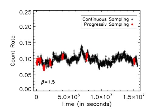
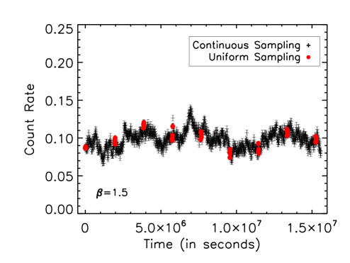
Figure 6.— Simulated continuously sampled AGN lightcurves (black crosses) compared with the progressive (upper panel) and uniform (lower panel) sampling schemes marked by red circles.

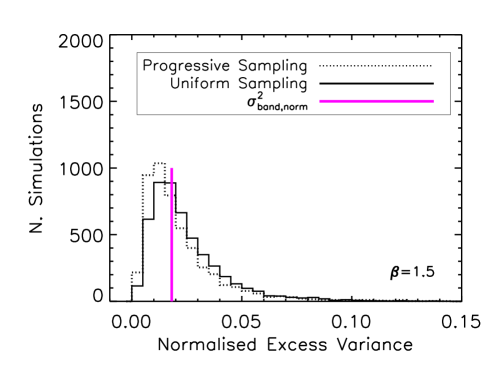
Figure 7.— The distribution of $\sigma^{2}_{\rm NXV}$ using the N=5000 simulated light curves with uniform (solid line) and progressive (dotted line) sampling. The vertical thick magenta line indicates $\sigma^{2}_{\rm band,norm}$, like in Fig. 3.

Table 3Properties and bias of the $\sigma^{2}_{\rm NXV}$ distributions for uniform and progressive sampling.

$\beta$	$\sigma^{2}_{\rm NXV}$	$\sigma^{2}_{\rm NXV}$	$b_{\rm uni}$	$b_{\rm pro}$
	Uniform	Progressive
1	0.035/0.016/1.61	0.033/0.015/1.38	0.97	1.02
1.5	0.025/0.019/2.27	0.022/0.020/5.21	0.73	0.82
2	0.018/0.018/3.42	0.016/0.019/5.55	0.46	0.51
2.5	0.013/0.016/3.63	0.012/0.018/6.24	0.28	0.30
3	0.011/0.015/4.07	0.010/0.016/6.00	0.15	0.16

Figure 7 shows the $\sigma^{2}_{\rm NXV}$ distribution for the uniform ($\sigma^{2}_{\rm NXV,uni}$; solid line) and progressive sampling scheme ($\sigma^{2}_{\rm NXV,pro}$; dotted line), derived from the 5000 simulations in the case of a PSD with $\beta=1.5$. The vertical solid line indicates $\sigma^{2}_{\rm band,norm}$ for $\beta=1.5$.

The mean, standard deviation and skewness of the distributions, as well as the bias values, are listed in Table 3. The standard deviations are similar for both sampling schemes. The skewness parameters indicate that the distributions are asymmetric. Skewness is larger in the case of progressive sampling. The mean, standard deviation and skewness of the $\sigma^{2}_{\rm NXV,uni}$ distributions are very similar to the same parameters of the $\sigma^{2}_{\rm NXV,cont}$ distributions. This is an interesting result, and shows that, even if we do not sample the time series continuously, as long as the sampling is uniform, the statistical properties of the derived normalized excess variance will be very similar to the properties of the normalized excess variance computed from a continuously sampled light curve (of similar length). Open (green) diamonds and filled (blue) diamonds in Figure 5 indicate the bias, $b$, of the $\sigma^{2}_{\rm NXV,uni}$ and of $\sigma^{2}_{\rm NXV,pro}$ distributions. The fact that it is difficult to discriminate between the filled squares and the open diamonds in this plot indicates clearly that the bias factors are identical in the case of the continuously sampled and the unevenly sampled lightcurves, when data are sampled uniformly.

This result shows that in general the sampling pattern is as important as, if not more important, than the total number of data points. The different patterns analyzed here and in Sec.4 have approximately the same total number of points (e.g. total exposure time) but different number of effectively independent (clusters of) points: the sparse pattern has only two independent clusters, the progressive one 5-6 independent clusters, while the uniform one samples the maximum number (9) of independent clusters and thus samples better the largest-amplitude/ longest-timescale variability trends (which dominate contributions to $\sigma^{2}_{NXS}$). Clearly in some instances, if a more detailed analysis than just the measure of the total variance, is required (such as the detailed study of the PSD), sampling more timescales as done by the progressive pattern may be preferable.

Finally, also in the analysis of the different sampling patterns, we verified that using the maximum-likelihood approach yields the same results as using the excess variance, as already found for the sparse sampling case discussed in Sec. 4.

5.2. Bias Dependence on the source flux

Table 4Statistical properties (mean/standard deviation/skewness) and bias of $\sigma^{2}_{\rm NXV}$ as a function of S/N ratio for $\beta=1.5$

.

Count Rate	$\frac{S}{N}$	Flux	$\sigma^{2}_{\rm NXV}$	$\sigma^{2}_{\rm NXV}$	$b_{\rm con}$	$b_{\rm spa}$
cnt s-1		(erg s-1cm-2)	Continuous	Sparse
0.1	25	6.25 $\times 10^{-13}$	0.025/0.016/2.42	0.018/0.023/4.94	0.75	1.0
0.05	22.6	3.12 $\times 10^{-13}$	0.025/0.016/2.53	0.018/0.024/5.36	0.75	1.0
0.01	6.3	6.25 $\times 10^{-14}$	0.025/0.016/2.52	0.017/0.025/5.85	0.75	1.1
0.005	3.4	3.12 $\times 10^{-14}$	0.025/0.017/2.68	0.017/0.033/4.03	0.75	1.1
0.002	1.4	1.25 $\times 10^{-14}$	0.025/0.024/1.16	0.015/0.11/0.94	0.75	1.2
0.001	0.8	6.25 $\times 10^{-15}$	0.025/0.070/ 0.34	0.014/0.43/0.96	0.75	1.3

We also examined whether the bias depends on the source flux (or more precisely, on the signal-to-noise ratio of the source) as a result of the increased white noise introduced by Poisson fluctuations, as the S/N ratio decreases. To estimate such effects, we simulated lightcurves assuming different average count rates, corresponding to fluxes smaller than the one of the source n.68, as is the case for the bulk of the AGN population detected in the CDFS. Conversion factors from counts to fluxes were calculated assuming a power law spectrum with $\Gamma=1.4$ and $N_{\rm H}=8\times 10^{19}$ cm^-2.

In Table 4 we list the statistical properties of the $\sigma^{2}_{\rm NXV,cont}$ and $\sigma^{2}_{\rm NXV,sparse}$ distributions in the case of a $\beta=1.5$ PSD, using the 5000 simulations in the case of the XMM-CDFS observation pattern. Our results show that the statistical properties of the $\sigma^{2}_{\rm NXV,cont}$ and $\sigma^{2}_{\rm NXV,sparse}$ distributions do not depend on the S/N of the lightcurve, as long as S/N $\geq 3$. Obviously, the uncertainty of the individual normalized excess variance measurements cannot be reduced just by increasing the S/N ratio of the lightcurve (say by increasing its bin size).

At smaller S/N ratios, the standard deviation of both distributions increases. This is an important result, specially in the case of continuously sample lightcurves. Fixed confidence intervals for the variance estimates (like the ones in Table 1 of Vaughan et al, 2003) should only be used for “bright” sources, where the S/N ratio of the available lightcurves is larger than 3. In the case of the sparsely sampled lightcurves, the standard deviation of the distribution becomes so large that the use of individual $\sigma^{2}_{\rm NXV,sparse}$ estimates will be meaningless. The bias of $\langle$$\sigma^{2}_{\rm NXV,sparse}$$\rangle$ increases as well, although we cannot be certain whether this is a real effect, or it is due to the fact that the standard deviation of the distribution has increased significantly, and as a result more simulations may be necessary in order to establish its mean reliably. We verified that the same result holds for all the PSDs we considered in the previous sections as well.

5.3. A simple prescription to estimate the bias of the sample excess variance

As we mentioned above, in the case of red-noise lightcurves, power leakage from lower frequencies, outside the sampled range, will result in $\sigma^{2}_{\rm NXV,cont}$ to be a biased estimate of $\sigma^{2}_{\rm band,norm}$. As our results show, $\langle$$\sigma^{2}_{\rm NXV,cont}$$\rangle$ systematically overestimates the intrinsic $\sigma^{2}_{\rm band,norm}$, for all PSDs. It seems then reasonable to assume that, the normalized excess variance still measures some kind of an intrinsic, normalized variance, and that:

$$\langle\sigma^{2}_{\rm NXV,cont}\rangle=\left[\int_{1/T^{\prime}_{\rm max}}^{1/T_{\rm min}}PSD(\nu)d\nu\right]/\mu^{2}$$ (8)

where $T^{\prime}_{\rm max}>T_{\rm max}$, to account for the ”red-noise leakage” effects. Using the above equation, Eq. (4) for $\sigma^{2}_{\rm band,norm}$, and Eq. (6) for the definition of bias, we can show that the bias for continuously sampled lightcurves will be equal to:

$$b_{\rm cont}=\frac{T_{\rm min}^{(\beta-1)}-T_{\rm max}^{(\beta-1)}}{T_{\rm min}^{(\beta-1)}-{T^{\prime}_{\rm max}}^{(\beta-1)}}\approx\left(\frac{T_{\rm max}}{T^{\prime}_{\rm max}}\right)^{\beta-1},$$ (9)

where the final expression assumes that $T_{\rm max},T^{\prime}_{\rm max}\gg T_{\rm min}$. The above equation can also be written as:

$${\rm log}\left(\frac{T_{\rm max}}{T^{\prime}_{\rm max}}\right)=\frac{{\rm log}(b_{\rm cont})}{\beta-1}$$ (10)

Using the values of $b_{\rm cont}$ listed in Table 2 (for $\beta>1$) we found that $T_{\rm max}/T^{\prime}_{\rm max}=0.48$. The solid line in Figure 5 shows a plot of the function $b_{\rm cont.}=0.48^{(\beta-1)}$. The agreement between this line and the data in the case of continuous, uniform and even progressive sampling is reasonably good. The difference between the predicted bias and the one determined from the simulations explained in §3 in the case of continuous sampling is less than 9% for $1\leq\beta\leq 2.5$ and increases to 15% for $\beta=3$ (this is an indication that $T^{\prime}_{\rm max}$ itself may be a function of $\beta$).

These results suggest that, in the case of continuously sampled light curves, with no missing points, the bias to the normalized excess variance can be accounted for if we assume that power at all frequencies down to approximately half the lowest sampled frequency contributes to the observed variability in the light curve. It appears that, for any light curve length (i.e. for any $T_{max}$), $\sigma^{2}_{NXV,cont}$ measures $\sigma^{2}_{band,norm}$ plus an amount of power which is equal to the integral of the PSD from $1/T_{max}$ to $\sim 1/(2T_{max})$. Thus the overall PSD shape at frequencies below $1/T^{\prime}_{max}$ does not appear to affect significantly the bias of the normalized excess variance. As long as we use the local mean of the light curve in the estimation of the normalized excess variance, it is the variability components with frequencies “just” below $1/T_{max}$ that transfer power to the observed light curves, and not the components with frequencies much lower than $1/T_{max}$.

This result allows us to consider the cases when the PSD is not just a simple power law at all frequencies higher than $1/T^{\prime}_{max}$. For example, if there exists a frequency “break” in the PSD, where the slope changes from $\beta\sim 1$ (at low frequencies) to $\beta\sim 2$ at high frequencies (just like the AGN X-rays PSDs) then, our bias prescription could in principle work in this case as well, provided we can make an assumption about the PSD slope at frequencies below the lowest sampled frequency, $1/T_{max}$. If the break time scale is shorter than $T_{max}$, and one can assume that the PSD slope at frequencies below $1/T_{max}$, down to $1/T^{\prime}_{max}$, is $\sim-1$, then the bias of the normalized excess variance should be minimal. If on the other hand, the break time scale is larger than $T^{\prime}_{max}$, then we believe that the adoption of a factor $\sim 0.48$ (which is valid in the case of power-law like PSDs with $\beta=2$), should provide a reasonable estimate of the bias of the normalized excess variance in this case. In general, as long as the PSD has a power-law shape of slope $\beta$ at frequencies below $1/T_{max}$, down to $1/T^{\prime}_{max}(=2.1T_{max})$, then a rough correction for the bias of the normalized excess variance (in the case of continuous sampled lightcurves) could be given by:

$$\sigma^{2}_{\rm NXV,cont}({\rm bias-corr.})=\sigma^{2}_{\rm NXV,cont.}\times 0.48^{(\beta-1)}$$ (11)

where $1\leq\beta\leq 3$. Strictly speaking, we have demonstrated that this is the case when the PSD has a simple, power-law like shape at all frequencies down to $1/T^{\prime}_{max}$, but we believe that this prescription should work reasonably well, even if the PSD slope steepens (changes) at frequencies higher than $1/T_{max}$.

In the case of discontinously sampled lightcurves, there will be timescales that are not sampled “properly”. Therefore, it seems reasonable to assume that, in this case, the normalized excess variance should be an estimate of the contribution to the total normalized variance of only these variability components that have been sampled. However, it is not easy to determine the longest and shorter time scales that have not been sampled in the observed lightcurve, as this depends on the sampling pattern in a complicated way. Our results indicate that, even if there is a large percentage of missing points (in the case of “uniform sampling” we discussed in Section 5.1, the percentage of missing points is almost 97%), the bias of the normalized excess variance should be almost equal to the bias of $\sigma^{2}_{\rm NXV,cont}$, as long as the data have been sampled in a quasi-evenly pattern.

In the case of the most extreme sampling pattern (for example when the data have been sampled only at the beginning and the end of the observing window), the bias of the excess normalized variance is larger than $b_{\rm cont}$ by a factor of $\sim 1.3$ in the case when $\beta\sim 1-1.5$. It then becomes almost equal to $b_{\rm cont}$ for PSDs with $\beta>2$. The dashed line in Figure 5 indicates the $b_{\rm cont}$ line multiplied by a factor of 1.3 for PSDs with slopes less than 2. The difference of the ”predicted” and observed bias factors is less than 10%.

We remind the reader that aliasing is not explicitly included in the bias values quoted above, and is not accounted for in equation 11. This approach is correct for most PSD slopes and typical sampled timescales, as the results will differ only if the slope is $\beta\lesssim 1$ at the maximum sampled frequency (e.g. cases where the PSD is very flat or we are only sampling long timescales below the “break” frequency). In particular for $\beta=1$ the bias will be reduced by $5-10\%$ with respect to the values quoted above, depending on the exact sampling pattern.

6. Excess Variance measurements in practice

In the previous sections we provided prescriptions to correct for the bias of $\sigma^{2}_{\rm NXV,cont}$ and $\sigma^{2}_{\rm NXV,sparse}$. However, although multiplication of the sampled normalized excess variance with the appropriate factors (see Eq. (11)) can result in an unbiased measurement of $\sigma^{2}_{\rm band,norm}$, given the large width of the distribution functions of these estimates, each individual $\sigma^{2}_{\rm NXV}$ measurement will still be a highly unreliable estimate of $\sigma^{2}_{\rm band,norm}$. This is particularly true for the case of sparsely sampled light curves.

Figure 8.— Bias distribution (of individual measurements) based on a set of 5000 simulated AGN lightcurves such as shown in Fig. 1, reproducing the continuous and sparse sampling pattern of the XMM-Newton observation of the CDFS.

To demonstrate this issue, the solid and dot-dashed lines in Figure 8 indicate the bias distribution of individual measurements (i.e. the bias as defined in Eq. 7 but without using an average value for $\sigma^{2}_{\rm NXV}$) from the continuously and sparsely sampled 5000 simulated lightcurves for the case of an intrinsic power-law PSD with $\beta=1.5$. These distributions convey the same information as the $\sigma^{2}_{\rm NXV,cont}$ and $\sigma^{2}_{\rm NXV,sparse}$ distributions, which are plotted in Figure 3, and the same comments about their width, and asymmetry, hold for them as well. But perhaps by plotting the distribution of the ”bias” factors, it becomes clearer that extreme care should by employed when inferring variability parameters from single observations of AGN, particularly if the lightcurves are sparsely sampled, in a non-uniform pattern. Although in the continuous sampling case most of the measurements are within a factor of $\sim 2$ from the intrinsic excess variance, in the sparse sampling 40%, 30% and 20% of the measurements have a bias larger than 2, 3 and 4, respectively. Even if the normalized excess variance distributions were multiplied by the appropriate bias factors so that their mean would be close to the intrinsic $\sigma^{2}_{\rm band,norm}$, individual $\sigma^{2}_{\rm NXV,sparse}$ estimates may still be significantly different than the intrinsic value.

We show below that, in order to derive a more robust estimate of the intrinsic source variance, we need to collect repeated observations of the same source or to use large samples of sources (assuming they have the same variability properties) in order to compute ”ensemble” estimates, which have more favourable statistical properties.

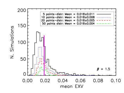
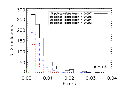
Figure 9.— Upper panel: Distribution of $\sigma^{2}_{\rm NXV}$ (eq. (12)) estimated by binning 5000 simulated excess variance (adopting the XMM sampling pattern, in groups of 5, 10 20 and 50 points (according to the legend). The inset shows the mean values of the binned distributions and their standard deviation, while the vertical thick magenta line shows the intrinsic variance $\sigma^{2}_{\rm band,norm}$. The simulations are performed by assuming a count rate of 0.1 cnt s^-1 and $\beta$ = 1.5. Lower panel: Distribution of the errors on $\overline{\sigma^{2}_{\rm NXV}}$ estimated from Eq. (13). The inset reports the mean values of the distributions for the different binning.

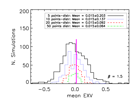
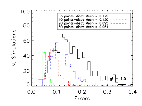
Figure 10.— As Figure 9 but for 0.001 cnt s^-1.

6.1. The Ensemble Excess Variance Estimates

We binned the 5000 simulated values of $\sigma^{2}_{\rm NXV,sparse}$ obtained by using the XMM pattern as described in §3 with $\beta=1.5$ in groups of $n=5,10,20,$ and 50 points. For each bin we estimated the ”mean-$\sigma^{2}_{\rm NXV}$”,

$$\overline{\sigma^{2}_{\rm NXV}}=\sum_{i=1}^{n}\sigma^{2}_{\rm NXV,\textit{i}}/n$$ (12)

and its “error”:

$$err(\overline{\sigma^{2}_{\rm NXV}})=\sqrt{\sum_{i=1}^{n}[\sigma^{2}_{\rm NXV,\textit{i}}-\overline{\sigma^{2}_{\rm NXV}}]/[n(n-1)]}.$$ (13)

Note that we dropped the subscript sparse in the equations above, as our results are applicable to the case of the continuously sampled lightcurves as well. The distributions of the 5, 10, 20 and 50-points binned $\overline{\sigma^{2}_{\rm NXV}}$ are shown in the upper panel of Figure 9 for a count rate of 0.1 cnt s^-1 (S/N=25) and $\beta=1.5$. The numbers in the inset window in this panel indicate the mean and standard deviation of each distribution. The mean of these distributions is identical to the mean of the $\sigma^{2}_{\rm NXV,sparse}$ distribution in the case when $\beta=1.5$, but their standard deviation is significantly smaller than the standard deviation of $\sigma^{2}_{\rm NXV,sparse}$  and the distributions are more symmetric. In fact, a Kolmogorov-Smirnov test performed on the 5, 10, 20 and 50-points mean-$\sigma^{2}_{\rm NXV}$ distributions indicates that only for the 5-points grouping we can reject the hypothesis of Gaussian distribution at $>95\%$ level.

Figure 9 (lower panel) shows the distribution of $err(\overline{\sigma^{2}_{\rm NXV}})$. The mean value of these distributions, which are quoted in the inset window, are almost identical to the standard deviation of the $\overline{\sigma^{2}_{\rm NXV}}$ distributions for $n\geq 10$. We verified that this is the case irrespective on the PSD slope $\beta$. This shows that the error on $\overline{\sigma^{2}_{\rm NXV}}$, calculated using Eq. (13), is indeed representative of the true scatter of these values around their mean. Therefore, when binning the individual $\sigma^{2}_{\rm NXV}$ estimates in practice, we can estimate the intrinsic uncertainty on $\overline{\sigma^{2}_{\rm NXV}}$ directly from the scatter of the individual points around $\overline{\sigma^{2}_{\rm NXV}}$ in each bin.

Similar results hold if we assume lightcurves with low S/N ratio. In Figure 10 we present the distribution of the 5, 10, 20 and 50-points $\overline{\sigma^{2}_{\rm NXV}}$ values, in the case of a lightcurve with a signal-to-noise ratio of 0.8 (i.e. $\sim 30$ times smaller than the S/N ratio of the object we considered above). Their mean values are very similar to the mean of the respective distributions for brighter sources. Their standard deviation, for $n\geq 20$, is at least 5 times smaller than the standard deviation of the distribution of the individual $\sigma^{2}_{\rm NXV,sparse}$ estimates (as listed in the bottom row of Table 4). Therefore, binning the individual excess variance estimates of faint sources (S/N$\sim 1$) by more than $n=20$, allows to retrieve and constrain much better the intrinsic “signal”. In addition, the 10, 20 and 50-points $\overline{\sigma^{2}_{\rm NXV}}$ distributions are approximately Gaussian, and their standard deviation is well approximated by the error of each binned estimate (for $n\geq 10$).

But of course, working with faint sources comes at a price. The standard deviation of the $n\geq 10$ $\overline{\sigma_{\rm NXV}^{2}}$ distributions for faint sources is $\sim 16-18$ times larger than the standard deviation of the respective distributions for brighter objects. Our results indicate that, for a $\sim 3\sigma$ detection of the variability amplitude amplitude in the case of lightcurves with S/N ratio $\sim 1$, one will need to bin at least 50 individual normalized excess variance estimates.

Table 5Statistical properties (mean/standard deviation/skewness) and bias of $\sigma^{2}_{\rm NXV}$ as a function of S/N ratio for a future mission described in §7

Mcr	$\frac{S}{N}$	Source Flux	$\sigma^{2}_{\rm NXV}$	$\sigma^{2}_{\rm NXV}$	$b_{\rm con}$	$b_{\rm spa}$
cnt s-1		(erg s-1cm-2)	Continuous	Sparse
0.1	38	$4\times 10^{-14}$	0.025/0.016/2.43	0.024/0.019/2.33	0.73	0.76
0.01	9.3	$4\times 10^{-15}$	0.025/0.016/2.43	0.024/0.021/1.98	0.73	0.75
0.005	7.2	$2\times 10^{-15}$	0.025/0.017/2.20	0.023/0.03/1.54	0.73	0.79
0.002	3.9	$8\times 10^{-16}$	0.025/0.025/1.18	0.020/0.13/1.38	0.73	0.91
0.001	2.7	$4\times 10^{-16}$	0.025/0.073/0.49	0.020/0.49/1.51	0.74	0.91

7. Constraints on the observing strategy of future X-ray surveys

Several missions have been proposed over the past few years to study high redshift AGNs; most of these are designed to have larger effective area than current X-ray missions, wider Field-of-View (FOV) and, depending on the planned orbit, lower background. For instance the International X-ray Observatory (IXO, Barcons et al., 2011) and its evolution Athena, the Wide Field X-ray Telescope (WFXT, Murray et al., 2010), all represent missions capable of performing AGN surveys with higher speed than Chandra or XMM. The results discussed in the previous sections allow to explore the capabilities of such future X-ray missions in the time domain. In particular we examine the expectations for deep, wide-area surveys, which will allow to probe the highest redshift and faintest AGN populations at the expense of a continuous temporal coverage.

To investigate the capabilities of such missions in measuring AGN variability, we present here the performance of a mission with 1 m² effective area, 1 sq.deg. FOV and the low background allowed by a low earth orbit, very similar to the WFXT design (Rosati et al., 2010). This results in a large number of moderate and high redshift AGN (see e.g. Paolillo et al., 2011). We used a total observing time of $\sim 400$ ks and we evaluated the performance that can be expected assuming a uniform sampling scheme very similar to the one presented in §5.1 (although not identical to the due to the WFXT survey constraints). Figures 11 represents an example of a possible observing scheme for the survey, where observations of 50 ks each are spread evenly over $\sim 6$ months and the corresponding excesses variance and bias distributions, respectively.

Figure 11.— Simulated AGN lightcurve, sampled in 50 ks observations spread uniformly on $\sim 6$ months, as expected from future large effective area mission such as those described in the text.

Figure 12.— As Figure 9 for a future mission with the characteristics and sampling pattern described in §7, assuming a mcr of 0.1 cnt s^-1.

In order to verify the performance of such type of mission for faint AGN populations, we explored the dependence of the measured excess variance on different values of the source mean count rate. The results are summarized in Table 5. The results are consistent with the findings shown in §5.1 (Table 4) but now we are able to measure variability with comparable accuracy at flux levels more than one order of magnitude lower than XMM, using approximately the same observing time, thus allowing variability studies for hundreds of AGN per square degree. Such good performances are due in part to the larger effective area, and in part to the low background made possible by the considered low-earth orbital configuration. We also notice that fortuitously, the bias actually improves at low count rates using such uniform sampling scheme, as the lost power better compensates the leakage coming from low frequencies.

8. Summary and Conclusions

In this paper we studied the statistical properties of $\sigma^{2}_{\rm NXV}$ and its performance in the case of lightcurves with an intrinsic ”red-noise” PSD. Strictly speaking, our results are valid in the case of Gaussian light curves, which remain only weakly non-stationary, on time scales of decades and shorter. Regarding the “stationarity” of the variability process, this may not be such a restrictive assumption, if the emission mechanism(s) in most of the AGN we observe has reached a “stable” state, i.e. statistical properties like the intrinsic mean flux, variance as well as the covariance at any two time points, may indeed remain constant, over time scales of the order of hundred of years or many decades. However, more work is necessary to investigate what will be the effects on our results if the AGN light curves are non-Gaussian.

Red-noise PSDs are common in many astrophysical time variable phenomena. In particular, the radio, optical and X-ray AGN lightcurves do show a ”red-noise” behaviour. We performed detailed Monte Carlo simulations, assuming PSD slopes between 1 and 3, and we considered the case of continuously and sparsely sampled lightcurves, assuming various sampling patterns, and various S/N ratios. Our results can be summarized as follows:

1. The statistical properties of $\sigma^{2}_{\rm ML}$ and $\sigma^{2}_{\rm NXV}$ are identical. Therefore, given the fact that it is easier to compute $\sigma^{2}_{\rm NXV}$, we propose its use for the study of the variability amplitude of the observed lightcurves.

2. We study in detail the bias of the normalized excess variance. If the intrinsic mean of the lightcurve were known in advance, then $\sigma^{2}_{\rm NXV}$ is an unbiased estimate of the intrinsic source variance normalized to the mean squared, even in the case of sparsely sampled light curve.

3. However, in most cases the intrinsic mean is unknown. In this case, our results show that $\sigma^{2}_{\rm NXV}$ is a biased estimate of $\sigma^{2}_{\rm band,norm}$  even in the case of continuously sampled lightcurves. The bias depends on the PSD slope, $\beta$, and increases as the PSD slope steepens. As long as $\beta$ is known in advance, or “red-noise” PSD models are fitted to the observed $\sigma^{2}_{\rm NXV}$ values, multiplication of the sampled $\sigma^{2}_{\rm NXV,cont}$ values by a factor equal to $0.48^{\beta-1}$ will result into estimates whose mean value will be within $\sim 15$% of the intrinsic $\sigma^{2}_{\rm band,norm}$.

4. The bias depends on the sampling pattern as well. However, even if there are many “missing” data points, the bias remains the same as in the case of the continuously sampled lightcurves, as long as the data are sampled uniformly over the observing period. In fact in general the sampling pattern is as important as, if not more important, than the total number of data points: the number of effectively independent (clusters of) points is the primary factor affecting the estimate of the total variance in cases where the variability amplitude is dominated by the longest timescales. In the extreme sampling patterns (like for example when most of the data points were obtained at the start and at the end of the observing period) we suggest that the bias factor we mentioned above is multiplied by 1.3 in the case when $1\leq\beta\leq 2$. At steeper PSDs, the main factor that determines $b$ is the PSD slope and not the sampling pattern.

5. Aliasing effects are negligible except for very flat PSD slopes with $\beta\lesssim 1$. Even for $\beta=1$ the correction is small and amounts to an increase of $5-10\%$ on the measured variance (and a corresponding decrease in the bias factor) depending on the sampling pattern. However aliasing is due to the PSD slope at the highest sampled frequency and thus this additional correction is needed only for cases where the PSD is very flat or if we are only sampling long timescales below the break frequency.

6. Individual $\sigma^{2}_{\rm NXV}$ measurements should be treated with extreme care, even if the “bias correction” recipe we mentioned above is applied to them. Their distribution has a large width, and is highly asymmetric, even in the case of continuously sampled lightcurves. The ratio of the distribution’s width over its mean, and the skewness of the $\sigma^{2}_{\rm NXV}$ distribution increase with $\beta$. This is a well know result of Vaughan et al. (2003). However, we find that the confidence limits provided by these authors most probably do not apply in the case of lightcurves with a S/N ratio less than 3.

7. For a given $\beta$, the width and asymmetry of the $\sigma^{2}_{\rm NXV}$ distribution increases significantly in the case lightcurves which are sparsely sampled, in a non-uniform pattern. Therefore, individual $\sigma^{2}_{\rm NXV}$ measurements are even more unreliable in this case. We do not recommend their use, specially in the case of extreme sampling patterns, and S/N ratios smaller than 3.

8. Based on our results, we strongly recommend the use of “ensemble” $\sigma^{2}_{\rm NXV}$ estimates in practice. These estimates should be preferred in the case when multiple lightcurves of the same object, or many lightcurves of objects with the same properties, are available. If there are $n\geq 20$ of such lightcurves, the distribution of the mean-$\sigma^{2}_{\rm NXV}$ (as defined by Equation 12) will be quite symmetric (and well approximated by a Gaussian), and its standard deviation will be well approximated by the error of the mean-$\sigma^{2}_{\rm NXV}$(given by Equation 13). This is result is valid for all PSD slopes, irrespective of the sampling pattern (i.e. whether the lightcurves are continuously or sparsely sampled), as long as the individual lightcurves have a S/N ratio $\geq 3$

9. At lower S/N ratio lightcurves, we recommend the use of the mean-$\sigma^{2}_{\rm NXV}$, but with $n\geq 50$.

The normalized excess variance is a useful tool to characterize the variability amplitude of astrophysical sources in cases when the available lightcurves cannot be used to estimate the PSD of as source (i.e. it is short and/or has many gaps). We believe that our results will be helpful to future studies which employ X-ray $\sigma^{2}_{\rm NXV}$ measurements to measure the BH mass of an AGN (both in the case of continuously and sparsely sampled lightcurves). The results presented in this work will be extremely useful in an era of rapidly growing (optical, radio, IR etc.) sky surveys, which often include timing informations despite the fact that a temporal strategy has not been specifically accounted for in planning the survey. In particular we showed that for a future X-ray mission, a properly designed observing strategy may allow to measure variability for hundreds of sources per square degree. Such dataset would largely overlap with the spectroscopic sample (e.g. Gilli et al., 2011), thus resulting thousand of AGNs with both temporal and spectroscopic informations. Since the individual variance estimates will still be affected by significant uncertainties, a large dataset will be essential in order to constrain the average timing properties of high redshift AGNs (provided that the AGN population shares the same intrinsic properties), and investigate their dependence of other source parameters (like spectral slope, luminosity etc). Several dedicated timing missions have also been proposed in the X-ray regime such as LOFT (Feroci et al. 2010). Our results are valid in such cases as well, as its instruments will provide data with sampling patterns close to the continuous (large area monitor) or uniform (wide-field monitor) cases explored here. More in general, our results will apply to any source characterized by red-noise variability, and can thus be useful in the estimation of the variability amplitude of sources that will result from multi-epoch and time-domain surveys such as those provided by e.g. Pan-STARRS and LSST.

References

- (1) Alexander, D. M., et al. 2003, ApJ, 126, 539
- (2) Almaini, O., et al., 2000, MNRAS, 315, 325
- Barcons et al. (2011) Barcons, X., Barret, D., Bautz, M., et al. 2011, arXiv:1102.2845
- Brandt & Hasinger (2005) Brandt, W. N., & Hasinger, G. 2005, ARA&A, 43, 827
- (5) Brunner, H., Cappelluti, N., Hasinger, G., Barcons, X., Fabian, A. C., Mainieri, V., & Szokoly, G. 2008, A&A, 479, 283
- Comastri et al. (2011) Comastri, A., et al. 2011, A&A, 526, L9
- Edelson et al. (2002) Edelson, R., Turner, T. J., Pounds, K., Vaughan, S., Markowitz, A., Marshall, H., Dobbie, P., & Warwick, R. 2002, ApJ, 568, 610
- Feroci et al. (2010) Feroci, M., et al. 2010, SPIE Conference Proceedings, 7732, 57
- Giacconi et al. (2002) Giacconi, R., et al., 2002, ApJS, 139, 369
- Gierlinski, Nikolajuk & Czerny (2008) Gierlinski, M., Nikołajuk, M., Czerny, B., 2008, MNRAS, 383, 741
- Gierliński et al. (2008) Gierliński, M., Middleton, M., Ward, M., & Done, C. 2008, Nature, 455, 369
- Gilli et al. (2011) Gilli, R., et al. 2011, Memorie della Societa Astronomica Italiana Supplementi, 17, 85
- Gonzalez-Martini et al. (2011) Gonzalez-Martin et al, 2011, A&A, 526, 132
- González-Martín & Vaughan (2012) González-Martín, O., & Vaughan, S. 2012, A&A, 544, A80
- Green et al. (1993) Green, A. R., McHardy, I., & Lehto, H. J., 1993, MNRAS, 265, 664
- Hasinger et al. (1993) Hasinger, G., et al. 1993, A&A, 26, 275
- Kataoka et al. (2001) Kataoka, J., Takahashi, T., Wagner, S. J., Iyomoto, N. , Edwards, P. G. , Hayashida, K. et al., 2001, ApJ 560, 659
- Koerding et al. (2007) Koerding, E. G., et al. 2007, MNRAS, 380, 301
- Lawrence & Papadakis (1993) Lawrence, A. & Papadakis, I. E. , 1993, ApJ, 414, 85
- Luo et al. (2008) Luo, B., et al. 2008, ApJS, 179, 19
- Markowitz et al. (2003) Markowitz, A., Edelson, R., Vaughan, S., et al. 2003, ApJ, 593, 96
- McHardy et al. (2004) McHardy, I. M. , Papadakis, I. E., Uttley, P., 2004, MNRAS,359, 348
- McHardy et al. (2005) McHardy, I. M. , Gunn, K. F., Uttley, P., & Goad, M. R., 2005, MNRAS, 359, 1469
- McHardy et al. (2006) McHardy, I. M., Koerding, E., Knigge, C., Uttley, P., Fender, R. P., 2006, Nature, 444, 730
- McHardy et al. (2007) McHardy, I. M. et al. 2007, MNRAS, 382, 985
- Murray et al. (2010) Murray, S. S. et al. 2010 in SPIE Conference Proceedings, Vol. 7732, 58
- Mushotzky et al. (2011) Mushotzky, R. F. et al. 2011, ApJL, 15, 6.
- Nandra et al. (1997) Nandra, K., George, I. M., Mushotzsky, R.F., et al., 1997, ApJ, 476, 70
- Nikolajuk, Papadakis & Czerny (2004) Nikolajuk, M., Papadakis, I. E., Czerny, B., 2004, MNRAS, 348, 207
- O’Neil et al. (2005) O’Neill P., et al. 2005, MNRAS, 358, 1405
- Paolillo et al. (2004) Paolillo, M., Schreier, E. J., Giacconi, R., Koekemoer, A. M., Grogin, N. A., 2004, ApJ, 611, 93
- Paolillo et al. (2011) Paolillo, M., et al. 2011, Memorie della Societa Astronomica Italiana Supplementi, 17, 97
- Papadakis et al. (2002) Papadakis, I.E., Brinkmann, W., Negoro, H., Gliozzi, M., 2002, A&A, 382, 1
- Papadakis et al. (2004) Papadakis, I.E., 2004, MNRAS, 348, 207
- Papadakis et al. (2008) Papadakis, I.E., Chatzopoulos, E., Athanasiadis, D. et al., 2008, A&A, 487, 475
- Ponti et al. (2012) Ponti. G., et al. 2012, A&A, 542, 83
- Turner et al. (1999) Turner, T. J., George, I. M., Nandra, K., & Turcan, D. 1999, ApJ, 524, 667
- Uttley et al. (2002) Uttley, P., McHardy, I.M., & Papadakis, I. E., 2002, MNRAS, 332, 231
- Rosati et al. (2010) Rosati, P., et al. 2011, Memorie della Societa Astronomica Italiana Supplementi, 17, 8
- Timmer & Koenig (1995) Timmer, J., Koenig, M., A&A, 1995, 300, 707
- (41) Uttley, P. & McHardy, I.M., 2005, MNRAS, 363, 286
- (42) Uttley, P., McHardy, I. M., Papadakis, I. E., 2002, MNRAS, 332, 231
- Vagnetti et al. (2011) Vagnetti, F., Turriziani, S., & Trevese, D. 2011, A&A, 536, A84
- Vaughan et al. (2003) Vaughan, S., Edelson, R., Warwick, R. S. and Uttley, P. 2003 MNRAS 345, 1271
- Xue et al. (2011) Xue, Y. Q., et al. 2011, ApJS 195, 10
- Zhang et al. (2011) Zhang, Y.-H. 2011, ApJ, 726, 21
- Zhou et al. (2010) Zhou, X. L., Zhang, S. N., Wang, D. X., Zhu, L., 2010, ApJ, 710, 16