Guaranteed clustering and biclustering via semidefinite programming
Abstract
Identifying clusters of similar objects in data plays a significant role in a wide range of applications. As a model problem for clustering, we consider the densest -disjoint-clique problem, whose goal is to identify the collection of disjoint cliques of a given weighted complete graph maximizing the sum of the densities of the complete subgraphs induced by these cliques. In this paper, we establish conditions ensuring exact recovery of the densest cliques of a given graph from the optimal solution of a particular semidefinite program. In particular, the semidefinite relaxation is exact for input graphs corresponding to data consisting of large, distinct clusters and a smaller number of outliers.
This approach also yields a semidefinite relaxation with similar recovery guarantees for the biclustering problem. Given a set of objects and a set of features exhibited by these objects, biclustering seeks to simultaneously group the objects and features according to their expression levels. This problem may be posed as that of partitioning the nodes of a weighted bipartite complete graph such that the sum of the densities of the resulting bipartite complete subgraphs is maximized. As in our analysis of the densest -disjoint-clique problem, we show that the correct partition of the objects and features can be recovered from the optimal solution of a semidefinite program in the case that the given data consists of several disjoint sets of objects exhibiting similar features. Empirical evidence from numerical experiments supporting these theoretical guarantees is also provided.
1 Introduction
The goal of clustering is to partition a given data set into groups of similar objects, called clusters. Clustering is a fundamental problem in statistics and machine learning and plays a significant role in a wide range of applications, including information retrieval, pattern recognition, computational biology, and image processing. The complexity of finding an optimal clustering depends significantly on the measure of fitness of a proposed partition, but most interesting models for clustering are posed as an intractable combinatorial problem. For this reason, heuristics are used to cluster data in most practical applications. Unfortunately, although much empirical evidence exists for the usefulness of these heuristics, few theoretical guarantees ensuring the quality of the obtained partition are known, even for data containing well separated clusters. For a recent survey of clustering techniques and heuristics, see [7]. In this paper, we establish conditions ensuring that the optimal solution of a particular convex optimization problem yields a correct clustering under certain assumptions on the input data set.
Our approach to clustering is based on partitioning the similarity graph of a given set of data. Given a data set and measure of similarity between any two objects, the similarity graph is the weighted complete graph with nodes corresponding to the objects in the data set and each edge having weight equal to the level of similarity between objects and . For this representation of data, clustering the data set is equivalent to partitioning the nodes of into disjoint cliques such that edges connecting any two nodes in the same clique have significantly higher weight than those between different cliques. Therefore, a clustering of the data may be obtained by identifying dense, in the sense of having large average edge weight, subgraphs of .
We consider the densest -partition problem as a model problem for clustering. Given a weighted complete graph and integer , the densest -partition problem aims to identify the partition of into disjoint sets such that the sum of the average edge weights of the complete subgraphs induced by these cliques is maximized. Unfortunately, the densest -partition problem is NP-hard, since it contains the minimum sum of squared Euclidean distance problem, known to be NP-hard [2], as a special case. In Section 2, we consider the related problem of finding the set of disjoint complete subgraphs maximizing the sum of their densities. We model this problem as a quadratic program with combinatorial constraints and relax to a semidefinite program using matrix lifting. This relaxation approach is similar to that employed in several recent papers [35, 43, 19], although we consider a different model problem for clustering and establish stronger recovery properties. We show that the optimal solution of this semidefinite relaxation coincides with that of the original combinatorial problem for certain program inputs. In particular, we show that the set of input graphs for which the relaxation is exact includes the set of graphs with edge weights concentrated on a particular collection of disjoint subgraphs, and provide a general formula for the clique sizes and number of cliques that may be recovered.
In Section 3, we establish similar results for the biclustering problem. Given a set of objects and features, biclustering, also known as co-clustering, aims to simultaneously group the objects and features according to their expression levels. That is, we would like to partition the objects and features into groups of objects and features, called biclusters, such that objects strongly exhibit features within their bicluster relative to the features within the other biclusters. Hence, biclustering differs from clustering in the sense that it does not aim to obtain groups of similar objects, but instead seeks groups of objects similar with respect to a particular subset of features. Applications of biclustering include identifying subsets of genes exhibiting similar expression patterns across subsets of experimental conditions in analysis of gene expression data, grouping documents by topics in document clustering, and grouping customers according to their preferences in collaborative filtering and recommender systems. For an overview of the biclustering problem, see [11, 18].
As a model problem for biclustering, we consider the problem of partitioning a bipartite graph into dense disjoint subgraphs. If the given bipartite graph has vertex sets corresponding to sets of objects and features with edges indicating expression level of each feature by each object, each dense subgraph will correspond to a bicluster of objects strongly exhibiting the contained features. Given a weighted bipartite complete graph and integer , we seek the set of disjoint bipartite complete subgraphs with sum of their densities maximized. We establish that this problem may be relaxed as a semidefinite program and show that, for certain program instances, the correct partition of can be recovered from the optimal solution of this relaxation. In particular, this relaxation is exact in the special case that the edge weights of the input graph are concentrated on some set of disjoint bipartite subgraphs. When the input graph arises from a given data set, the relaxation is exact when the underlying data set consists of several disjoint sets strongly exhibiting nonoverlapping sets of features.
Our results build upon those of recent papers regarding clusterability of data. These papers generally contain results of the following form: if a data set is randomly sampled from a distribution of “clusterable” data, then the correct partition of the data can be obtained efficiently using some heuristic, such as the -means algorithm or other iterative partitioning heuristics [32, 1, 42, 6], spectral clustering [31, 27, 40, 5], or convex optimization [3, 30, 26, 33]. Recent papers by Kolar et al. [28], Rohe and Yu [41], and Flynn and Perry [20] establish analogous recovery guarantees for biclustering; the latter two of these papers appeared shortly after the initial preprint release of this paper. Our results are of a similar form. If the underlying data set consists of several sufficiently distinct clusters or biclusters, then the correct partition of the data can be recovered from the optimal solution of our relaxations. We model this ideal case for clustering using random edge weight matrices constructed so that weight is, in expectation, concentrated heavily on the edges of a few disjoint subgraphs. We will establish that this random model for clustered data contains those previously considered in the literature and, in this sense, our results are a generalization of these earlier theoretical guarantees.
More generally, our results follow in the spirit of, and borrow techniques from, recent work regarding sparse optimization and, in particular, the nuclear norm relaxation for rank minimization. The goal of matrix rank minimization is to find a solution of minimum rank of a given linear system, i.e., to find the optimal solution of the optimization problem for given linear operator and vector . Although this problem is well-known to be NP-hard, several recent papers ([37, 13, 4, 24, 36, 12, 38, 34], among others) have established that, under certain assumptions on and , the minimum rank solution is equal to the optimal solution of the convex relaxation obtained by replacing with the sum of the singular values of , the nuclear norm . This relaxation may be thought of as a matrix analogue of the norm relaxation for the cardinality minimization problem, and these results generalize similar recovery guarantees for compressed sensing (see [15, 14, 16]). For example, the nuclear norm relaxation is exact with high probability if is a random linear transform with matrix representation having i.i.d. Gaussian or Bernoulli entries and is the image of a sufficiently low rank matrix under . We prove analogous results for an instance of rank constrained optimization. To identify the densest complete subgraphs of a given graph, we seek a rank- matrix maximizing some linear function of , depending only on the edge weights of the input graph, subject to linear constraints. We will see that the optimal rank- solution is equal to that obtained by relaxing the rank constraint to the corresponding nuclear norm constraint if the matrix is randomly sampled from a probability distribution satisfying certain assumptions.
2 A semidefinite relaxation of the densest -disjoint-clique problem
Given a graph , a clique of is a pairwise adjacent subset of . That is, is a clique of if for every pair of nodes . Let be a complete graph with vertex set and nonnegative edge weights for all . A -disjoint-clique subgraph of is a subgraph of consisting of disjoint complete subgraphs, i.e., the vertex sets of each of these subgraphs is a clique. For any subgraph of , the density of , denoted , is the average edge weight incident at a vertex in :
The densest -disjoint-clique problem concerns choosing a -disjoint-clique subgraph of such that the sum of the densities of the subgraphs induced by the cliques is maximized. Given a -disjoint-clique subgraph with vertex set composed of cliques , the sum of the densities of the subgraphs induced by the cliques is equal to
| (2.1) |
where is the characteristic vector of . In the special case that defines a partition of and for a given set of vectors in with maximum distance between any two points at most one, we have
where is the center of the vectors assigned to for all , since for this choice of . Here, and in the rest of the note, denotes the norm in . For this choice of , the densest -partition problem, i.e., finding a partition of such that the sum of densities of the subgraphs induced by is maximized, is equivalent to finding the partition of such that the sum of the squared Euclidean distances
| (2.2) |
from each vector to its assigned cluster center is minimized. Unfortunately, minimizing over all potential partitions of is NP-hard and, thus, so is the densest -partition problem (see [35]). It should be noted that the complexity of the densest -disjoint-clique subgraph problem is unknown, although the problem of minimizing over all -disjoint-clique subgraphs has the trivial solution of assigning exactly one point to each cluster and setting all other points to be outliers.
If we let be the matrix with th column equal to , we have We call such a matrix a normalized -partition matrix. That is, is a normalized k-partition matrix if the columns of are the normalized characteristic vectors of disjoint subsets of . We denote by the set of all normalized -partition matrices of . We should note that the term normalized -partition matrix is a slight misnomer; the columns of do not necessarily define a partition of into disjoint sets but do define a partition of into the disjoint sets given by the columns of and their complement. Using this notation, the densest -disjoint-clique problem may be formulated as the quadratic program
| (2.3) |
Unfortunately, quadratic programs with combinatorial constraints are NP-hard in general.
The quadratic program (2.3) may be relaxed to a rank constrained semidefinite program using matrix lifting. We replace each column of with a rank-one semidefinite variable to obtain the new decision variable The new variable has both rank and trace exactly equal to since the summands are orthogonal rank-one matrices, each with nonzero eigenvalue equal to 1. Moreover, since for all and all remaining components equal to where is equal to the number of nonzero entries of , we have
Thus, the matrix has row sum equal to one for each vertex in the subgraph of defined by the columns of and zero otherwise. Therefore, we may relax (2.3) as the rank constrained semidefinite program
| (2.4) |
Here denotes the cone of symmetric positive semidefinite matrices and denotes the all-ones vector in . The nonconvex program (2.4) may be relaxed further to a semidefinite program by ignoring the nonconvex constraint :
| (2.5) |
Note that a -disjoint-clique subgraph with vertex set composed of disjoint cliques defines a feasible solution of (2.5) with rank exactly equal to and objective value equal to (2.1) by
| (2.6) |
where is the characteristic vector of for all . This feasible solution is exactly the lifted solution corresponding to the cliques . This relaxation approach mirrors that for the planted -disjoint-clique problem considered in [3]. In [3], entrywise nonnegativity constraints can be ignored for the sake of computational efficiency due to explicit constraints forcing all entries of a feasible solution corresponding to unadjacent nodes to be equal to 0. Due to the lack of such constraints in (2.5), the nonnegativity constraints are required to ensure that the optimal solution of (2.5) is unique if the input data is sufficiently clusterable. Indeed, suppose that
where is the all-ones vector in . Then both
are positive semidefinite, have trace equal to , row sums bounded above by , and have objective value equal to . Therefore, the nonnegativity constraints are necessary to distinguish between these two solutions. We should also point out that the constraints of (2.5) are similar to those of the semidefinite relaxation used to approximate the minimum sum of squared Euclidean distance partition by Peng and Wei in [35], although with different derivation.
The relaxation (2.5) may be thought of as a nuclear norm relaxation of (2.4). Indeed, since the eigenvalues and singular values of a positive semidefinite matrix are identical, every feasible solution satisfies Moreover, since every feasible solution is symmetric and has row sums at most , we have for every feasible . Here , , and denote the matrix norms on induced by the , , and norms on respectively. This implies that every feasible satisfies since (see [23, Corollary 2.3.2]). Since is the convex envelope of on the set (see, for example, [37, Theorem 2.2]), the semidefinite program (2.5) is exactly the relaxation of (2.4) obtained by ignoring the rank constraint and only constraining the nuclear norm of a feasible solution. Many recent results have shown that the minimum rank solution of a set of linear equations is equal to the minimum nuclear norm solution, under certain assumption on the linear operator . We would like to prove analogous results for the relaxation (2.5). That is, we would like to identify conditions on the input graph that guarantee recovery of the densest -disjoint-clique subgraph by solving (2.5).
Ideally, a clustering heuristic should be able to correctly identify the clusters in data that is known a priori to be clusterable. In our graph theoretic model, this case corresponds to a graph admitting a -disjoint-clique subgraph with very high weights on edges connecting nodes within the cliques and relatively low weights on edges between different cliques. We focus our attention on input instances for the densest -disjoint-clique problem that are constructed to possess this structure. Let be a -disjoint-clique subgraph of with vertex set composed of disjoint cliques . We consider random symmetric matrices with entries sampled independently from one of two distributions , as follows:
-
•
For each , the entries of each diagonal block are independently sampled from a probability distribution satisfying and for all .
-
•
All remaining entries of are independently sampled from a probability distribution satisfying and for all .
That is, we sample the random variable from the probability distribution with mean if the nodes are in the same planted clique; otherwise, we sample from the distribution with mean . We say that such random matrices are sampled from the planted cluster model. We should note the planted cluster model is a generalization of the planted -disjoint-clique subgraph model considered in [3], as well as the stochastic block/probabilistic cluster model considered in [26, 33, 40]. Indeed, the stochastic block model is generated by independently adding edges within planted dense subgraphs with probability and independently adding edges between cliques with probability for some . The planted -disjoint-clique subgraph model is simply the stochastic block model in the special case that . Therefore, choosing and to be Bernoulli distributions with probabilities of success and , respectively, yields sampled from the stochastic block model.
The following theorem describes which partitions of yield random symmetric matrices drawn from the planted cluster model such that the corresponding planted -disjoint-clique subgraph is the densest -disjoint-clique subgraph and can be found with high probability by solving (2.5).
Theorem 2.1
Suppose that the vertex sets define a -disjoint-clique subgraph of the complete graph on vertices and let Let for all , and let . Let be a random symmetric matrix sampled from the planted cluster model according to distributions and with means and , respectively, satisfying
| (2.7) |
where is the Kronecker delta function defined by if and otherwise. Let be the feasible solution for (2.5) corresponding to defined by (2.6). Then there exist scalars such that if
| (2.8) |
then is the unique optimal solution for (2.5), and is the unique maximum density -disjoint-clique subgraph of corresponding to with probability tending exponentially to as .
Note that the condition (2.7) implies that if and otherwise. That is, if defines a partition of then the restriction that can be relaxed to . On the other hand, the condition (2.8) cannot be satisfied unless and . We now provide a few examples of satisfying the hypothesis of Theorem 2.1.
-
•
Suppose that we have cliques of size . Then (2.8) implies that we may recover the -disjoint-clique subgraph corresponding to if . Since the cliques are disjoint and contain nodes, we must have . Therefore, our heuristic may recover planted cliques of size .
-
•
On the other hand, we may have cliques of different sizes. For example, suppose that we wish to recover cliques of size and smaller cliques of size . Then the right-hand side of (2.8) must be at least Therefore, we may recover the planted cliques provided that , , and .
Although we consider a more general model for clustered data, our recovery guarantee agrees (up to constants) with those existing in the literature. In particular, the bound on the minimum size of the planted clique recoverable by the relaxation (2.5), , provided by Theorem 2.1 matches that given in [26, 33]. However, among the existing recovery guarantees in the literature, few consider noise in the form of diversionary nodes. As a consequence of our more general model, the relaxation (2.5) is exact for input graphs containing up to noise nodes, fewer than the bound, , provided by [3, Theorem 4.5].
3 A semidefinite relaxation of the densest -disjoint-biclique problem
Given a bipartite graph , a pair of disjoint independent subsets , is a biclique of if the subgraph of induced by is complete bipartite. That is, is a biclique of if for all . A -disjoint-biclique subgraph of is a subgraph of with vertex set composed of disjoint bicliques of . Let be a weighted complete bipartite graph with vertex sets , with matrix of edge weights . We are interested in identifying the densest -disjoint-biclique subgraph of with respect to . We define the density of a subgraph of to be the total edge weight incident at each vertex divided by the square root of the number of edges from to :
| (3.1) |
Note that the density of , as defined by (3.1), is not necessarily equal to the average edge weight incident at a vertex of , since the square root of the number of edges is not equal to the total number of vertices if or is not complete. The goal of the densest -disjoint-biclique problem is to identify a set of disjoint bicliques of such that the sum of the densities of the complete subgraphs induced by these bicliques is maximized. That is, we want to find a set of disjoint bicliques, with characteristic vectors , maximizing the sum
| (3.2) |
As in our analysis of the densest -disjoint-clique problem, this problem may be posed as the nonconvex quadratic program
| (3.3) |
By letting , we have , where
Using this change of variables, we relax to the rank constrained semidefinite program
| (3.4) |
where and are the blocks of with rows and columns indexed by and respectively. Ignoring the nonconvex rank constraints yields the semidefinite relaxation
| (3.5) |
As in our analysis of the densest -disjoint-clique problem, we would like to identify sets of program instances of the -disjoint-biclique problem that may be solved using the semidefinite relaxation (3.5). As before, we consider input graphs where it is known a priori that a -disjoint-biclique subgraph with large edge weights, relative to the edges of its complement, exists. We consider random program instances generated as follows. Let be a -disjoint-biclique subgraph of with vertex set composed of the disjoint bicliques . We construct a random matrix with entries sampled independently from one of two distributions as follows.
-
•
If , for some , then we sample from the distribution , with mean . If and are in different bicliques of , then we sample according to the probability distribution , with mean .
-
•
The probability distributions are chosen such that , .
We say that such are sampled from the planted bicluster model. Note that defines a feasible solution for (3.5) by
| (3.6) |
where are the characteristic vectors of and , respectively, for all . Moreover, has objective value equal to (3.2). The following theorem describes which partitions and of and yield random matrices drawn from the planted bicluster model such that is the unique optimal solution of the semidefinite relaxation (3.5) and is the unique densest -disjoint-biclique subgraph.
Theorem 3.1
Suppose that the vertex sets define a -disjoint-biclique subgraph of the complete bipartite graph . Let and . Let and for all and . Let be the feasible solution for (3.5) corresponding to given by (3.6). Let be a random matrix sampled from the planted bicluster model according to distributions and with means satisfying
| (3.7) |
Suppose that there exist scalars such that for all and
| (3.8) |
for all . Then there exist scalars depending only on and such that if
| (3.9) |
then is the unique optimal solution of (3.5) and is the unique maximum density -disjoint-biclique subgraph with respect to with probability tending exponentially to as tends to .
4 Proof of Theorem 2.1
This section comprises a proof of Theorem 2.1. The proof of Theorem 3.1 is essentially identical to that of Theorem 2.1, although with some modifications made to accommodate the different relaxation and lack of symmetry of the weight matrix an outline of the proof of Theorem 3.1 is given in Section 5.
4.1 Optimality Conditions
We begin with the following sufficient condition for the optimality of a feasible solution of (2.5).
Theorem 4.1
Note that is a strictly feasible solution of (2.5) for sufficiently small . Thus, Slater’s constraint qualification holds for (2.5). Therefore, a feasible solution is optimal for (2.5) if and only if it satisfies the Karush-Kuhn-Tucker conditions. Theorem 4.1 provides the necessary specialization to (2.5) of these necessary and sufficient conditions (see, for example, [10, Section 5.5.3] or [39, Theorem 28.3]).
Let be a -disjoint-clique subgraph of with vertex set composed of the disjoint cliques of sizes and let be the corresponding feasible solution of (2.5) defined by (2.6). Let and . Let . Let be a random symmetric matrix sampled from the planted cluster model according to and with means and . To show that is optimal for (2.5), we will construct multipliers , , , and satisfying (4.1), (4.2), (4.3), and (4.4). Note that the gradient equation (4.1) provides an explicit formula for the multiplier for any choice of multipliers and .
The proof of Theorem 2.1 uses techniques similar to those used in [3]. Specifically, the proof of Theorem 2.1 relies on constructing multipliers satisfying Theorem 4.1. The multipliers and will be constructed in blocks inherited from the block structure of the proposed solution . Again, once the multipliers and are chosen, (4.1) provides an explicit formula for the multiplier .
The dual variables must be chosen so that the complementary slackness condition (4.4) is satisfied. The condition is satisfied if and only if , since both and are desired to be positive semidefinite (see [44, Proposition 1.19]). Therefore, the multipliers must be chosen so that the left-hand side of (4.1) is orthogonal to the columns of . That is, we must choose the multipliers and such that , as defined by (4.1), has nullspace containing the columns of . By the special block structure of , this is equivalent to requiring to sum to for all and
The gradient equation (4.1), coupled with the requirement that the columns of reside in the nullspace of , provides an explicit formula for the multiplier . Moreover, the complementary slackness condition (4.3) implies that all diagonal blocks , , are equal to . To construct the remaining multipliers, we parametrize the remaining blocks of using the vectors and for all . These vectors are chosen to be the solutions of the system of linear equations defined by . As in [3], we will show that this system is a perturbation of a linear system with known solution and will use this known solution to obtain estimates of and .
Once the multipliers are chosen, we must establish dual feasibility to prove that is optimal for (2.5). In particular, we must show that and are nonnegative and is positive semidefinite. To establish nonnegativity of and , we will show that these multipliers are strictly positive in expectation and close to their respective means with extremely high probability. To establish that is positive semidefinite, we will show that the diagonal blocks of dominate the off diagonal blocks with high probability.
4.2 Choice of the multipliers and a sufficient condition for uniqueness and optimality
We construct the multipliers , and in blocks indexed by the vertex sets . The complementary slackness condition (4.4) implies that the columns of are in the nullspace of since if and only if for all positive semidefinite . Since is a multiple of the all-ones matrix for each , and all other entries of are equal to , (4.4) implies that the block must have row and column sums equal to for all . Moreover, since all entries of are nonzero, for all by (4.3).
To compute an explicit formula for , note that the condition is satisfied if
| (4.5) |
for all . Rearranging (4.5) shows that is the solution to the system
| (4.6) |
for all . We will use the Sherman-Morrision-Woodbury formula (see, for example, [23, Equation (2.1.4)]), stated in the following lemma, to obtain the desired formula for .
Lemma 4.1
Let be nonsingular and be such that . Then
| (4.7) |
We next construct . Fix such that . To ensure that and , we parametrize the entries of using the vectors and . In particular, we take
| (4.9) |
Here , where is the Kronecker delta function defined by if and otherwise. That is, we take to be the expected value of , plus the parametrizing terms and . The vectors and are chosen to be the solutions to the systems of linear equations imposed by the requirement that . As we will see, this system of linear equations is a perturbation of a linear system with known solution. Using the solution of the perturbed system we obtain bounds on and , which are used to establish that is nonnegative and is positive semidefinite.
Let
| (4.10) |
Note that the symmetry of implies that . Let be defined by and We choose and to be solutions of the system
| (4.11) |
for some scalar to be defined later. The requirement that the row sums of are equal to zero is equivalent to and satisfying the system of linear equations
| (4.12) |
for all . Similarly, the column sums of are equal to zero if and only if and satisfy
| (4.13) |
for all . Note that the system of equations defined by (4.12) and (4.13) is equivalent to (4.11) in the special case that . However, when , the system of equations in (4.11) is singular, with nullspace spanned by the vector . When is nonzero, each row of the system (4.11) has an additional term of the form . However, any solution of (4.11) for is also a solution in the special case that . Indeed, since is in the nullspace of the matrix
and , taking the inner product of each side of (4.11) with yields
Therefore, the unique solution of (4.11) also satisfies (4.12) and(4.13) for any such that (4.11) is nonsingular. In particular, note that (4.11) is nonsingular for . For this choice of , and are the unique solutions of the systems and , where and . Applying (4.7) with , and , yields
| (4.14) |
respectively. Finally, we choose , where and is a scalar to be chosen later.
In summary, we choose the multipliers , , as follows:
| (4.15) |
| (4.16) |
| (4.19) |
where is a scalar to be defined later, is defined as in (4.10), and are given by (4.14) for all such that . We choose according to (4.1). Finally, we define the block matrix in by
| (4.20) |
We conclude with the following theorem, which provides a sufficient condition ensuring that the proposed solution is the unique optimal solution for (2.5) and is the unique maximum density -disjoint-clique subgraph of corresponding to .
Theorem 4.2
Suppose that the vertex sets define a -disjoint-clique subgraph of the complete graph on vertices and let Let for all , and let . Let be a random symmetric matrix sampled from the planted cluster model according to distributions with means satisfying (2.7). Let be the feasible solution for (2.5) corresponding to defined by (2.6). Let and be chosen according to (4.15), (4.16), and (4.19), and let be chosen according to (4.1). Suppose that the entries of and are nonnegative. Then there exists scalar such that if then is optimal for (2.5), and is the maximum density -disjoint-clique subgraph of corresponding to . Moreover, if
| (4.21) |
for all such that , then is the unique optimal solution of (2.5) and is the unique maximum density -disjoint-clique subgraph of .
Proof: By construction, , , , and satisfy (4.1), (4.2), (4.3), and (4.4). Moreover, and are nonnegative by assumption. Therefore, it suffices to show that is positive semidefinite to prove that is optimal for (2.5). To do so, we fix and decompose as where
for some chosen such that is orthogonal to for all , and . Here, and in the rest of the note, the notation denotes the vector in with entries equal to those of indexed by . Similarly, the notation denotes the matrix with entries equal those of indexed by and respectively. We have
since is orthogonal to for all and, hence, . Therefore, if , then for all with equality if and only if . In this case, is optimal for (2.5). Moreover, is in the nullspace of for all by (4.4) and the fact that . Since if and only if , the nullspace of is exactly equal to the span of and has rank equal to .
To see that is the unique optimal solution for (2.5) if Assumption (4.21) holds, suppose, on the contrary, that is also optimal for (2.5). By (4.4), we have , which holds if and only if . Therefore, the row and column spaces of lie in the nullspace of . Since and , we may write as
| (4.22) |
for some . The fact that satisfies implies that
| (4.23) |
for all . Moreover, since , there exists some such that
| (4.24) |
Combining (4.23) and (4.24) shows that
contradicting Assumption (4.21). Therefore, is the unique optimal solution of (2.5) as required.
4.3 Nonnegativity of and in the planted case
We now establish that the entries of and are nonnegative with probability tending exponentially to as approaches for sufficiently small choice of in (4.15).
We begin by deriving lower bounds on the entries of . To do so, we will repeatedly apply the following theorem of Hoeffding (see [25, Theorem 1]), which provides a bound on the tail distribution of a sum of bounded, independent random variables.
Theorem 4.3 (Hoeffding’s Inequality)
Let be independent identically distributed (i.i.d.) variables sampled from a distribution satisfying for all . Let . Then
| (4.25) |
for all .
To show that for all with high probability, we will use the following lemma, which provides an upper bound on and for all such that , holding with probability tending to as tends to .
Lemma 4.2
There exists scalar such that for all such that with probability tending exponentially to as .
Proof: Fix such that . Without loss of generality, we assume that . The proof for the case when either or is equal to is analogous. We first obtain an upper bound on . By the triangle inequality, we have
| (4.26) |
Hence, to obtain an upper bound on , it suffices to obtain bounds on and . We begin with . Recall that we have
| (4.27) |
for each . Note that
Applying (4.25) with , and , shows that
| (4.28) |
with probability at least where . Next, applying (4.25) with and shows that
| (4.29) |
with probability at least where Finally, applying (4.25) with and (4.28) shows that
| (4.30) |
with probability at least . Combining (4.28), (4.29) and (4.30) and applying the union bound shows that
| (4.31) |
with probability at least By a similar argument, with probability at least
We next obtain an upper bound on and . We have
| (4.32) |
By (4.28) and the union bound, we have
| (4.33) | ||||
| (4.34) |
with probability at least . Moreover, applying (4.25) with and shows that
| (4.35) |
with probability at least , where Substituting (4.33) and (4.35) into (4.32), we have
| (4.36) |
for some scalar with probability at least by the union bound. Similarly,
| (4.37) |
with probability at least . Substituting (4.31) and (4.36) in (4.26) yields
| (4.38) |
for some scalar , with probability at least Similarly, there exists scalar such that
| (4.39) |
with probability at least Combining (4.38) and (4.39) and applying the union bound over all completes the proof.
As an immediate consequence of Lemma 4.2, is nonnegative with probability tending exponentially to for sufficiently large values of .
Corollary 4.1
Suppose that and satisfy (2.7). Then the entries of the matrix are nonnegative with probability tending exponentially to as approaches .
Proof: Fix , for some such that . Recall that
Therefore, since by (2.7), Lemma 4.2 implies that
for all sufficiently small and sufficiently large with probability tending exponentially to as , since at most one of and is equal to .
The following lemma provides a similar lower bound on the entries of .
Lemma 4.3
There exist scalars such that for all with probability tending exponentially to as .
Proof: Fix and . Recall that
Applying (4.25) with and yields
| (4.40) |
with probability at least . Moreover, (4.34) implies that
| (4.41) |
with probability at least . Combining (4.40) and (4.41) and applying the union bound shows that there exist scalars such that
with probability at least for sufficiently small choice of in (4.15). Applying the union bound over all completes the proof.
Note that Lemma 4.3 implies that with probability tending exponentially to as tends to . Therefore, , , constructed according to (4.15), (4.16), and (4.19) are dual feasible for (2.5) with probability tending exponentially to as if the left-hand side of (4.1) is positive semidefinite. The following lemma states the uniqueness condition given by (4.21) is also satisfied with high probability for sufficiently large .
Lemma 4.4
If then for all such that with probability tending exponentially to as .
Proof: Fix such that . Combining (4.28) and (4.35) shows that
with probability at least . Noting that this lower bound is positive if and applying the union bound over all choices of and completes the proof.
We have shown that constructed according to (4.15), (4.16), and (4.19) are dual feasible for (2.5) and the uniqueness condition (4.21) is satisfied with probability tending exponentially to as . In the next subsection, we derive an upper bound on the norm of and use this bound to obtain conditions ensuring dual feasibility of and, hence, optimality of for (2.5).
4.4 An upper bound on
In this section, we derive an upper bound on , which will be used to verify that the conditions on the partition imposed by (2.8) ensure that the -disjoint-clique subgraph of composed of the cliques is the unique maximum density -disjoint-clique of with respect to and can be recovered by solving (2.5) with probability tending exponentially to as . In particular, we will prove the following lemma.
Lemma 4.5
There exist scalars such that
| (4.42) |
with probability tending exponentially to as approaches .
This lemma, along with Theorem 4.2, Lemma 4.3, and Corollary 4.1, establishes Theorem 2.1. Indeed, if the right-hand side of (4.42) is bounded above by then Theorem 4.2, Lemma 4.3, and Corollary 4.1 imply that the -disjoint-clique subgraph given by is the densest -disjoint-clique subgraph corresponding to and can be recovered by solving (2.5).
The remainder of this section consists of a proof of Lemma 4.5. We decompose as where , , are by block matrices such that
To bound the norm of each matrix in this decomposition, we will make repeated use of the following bound on the norm of a random symmetric matrix (see [21], [4, Theorem 1]).
Theorem 4.4
Let be a random symmetric matrix with i.i.d. entries sampled from a distribution with mean and variance such that for all . Then with probability at least where depends only on .
We are now ready to compute the desired bound on . By Theorem 4.4, there exist such that with probability tending exponentially to as . Morever, we have It remains to obtain an upper bound on .
Note that by the triangle inequality. Recall that
for all . Applying Theorem 4.4, there exists such that
with probability tending exponentially to as . On the other hand, (4.28) implies that with probability at least . It follows that there exists scalar such that for all with probability tending exponentially to as . Therefore, with high probability, as required. This completes the proof of Lemma 4.5.
5 Proof of Theorem 3.1
5.1 Optimality conditions and choice of multipliers
We provide of a sketch of the proof of Theorem 3.1 here; many of the technical details are identical to those in the proof of Theorem 2.1 and are omitted. As before, we will establish that a proposed solution satisfies a set of sufficient conditions for optimality for (3.5), given by the following theorem, with high probability if the input graph satisfies the assumptions of Theorem 3.1.
Theorem 5.1
Let , …, denote the vertex sets of the -disjoint-biclique subgraph of the bipartite complete graph with vertex sets and of size and respectively. Let and . Let be a random nonnegative matrix sampled from the planted bicluster model according to distributions with means . Let , for all , and let , . Let and let for all . We assume that is equal to a scalar multiple of for all . That is, for some for all .
As before, we establish optimality of by constructing dual multipliers satisfying the assumptions of Theorem 5.1. The matrix and, hence, , , and will be constructed in blocks indexed by the vertex sets and . Note that the diagonal blocks of indexed by consist of multiples of the all-ones matrix and the remaining blocks are equal to . Therefore, by (5.4). Similarly, the block structure of implies that by (5.5) and for all by (5.6).
Since both and are assumed to be positive semidefinite matrices, the complementary slackness condition, , is equivalent to requiring the columns of to reside in the nullspace of . For each we choose so that is orthogonal to . In particular, it suffices to choose such that
| (5.8) |
for all . Rearranging (5.8) shows that is the solution to the system
| (5.9) |
for all . As before, the Sherman-Morrision-Woodbury formula yields an explicit formula for ; for each , applying (4.7) with , shows that
| (5.10) |
Similarly, choosing
| (5.11) |
forces the rows of to be orthogonal to the columns of for all . Note that for all . We choose for some scalar to be defined later to ensure that is nonnegative in expectation. Similarly, for all . Again, we choose for small enough to ensure that is nonnegative in expectation.
We next construct the multiplier . We set and parametrize using the vectors and for each . For each , let be the vector in such that and . We choose , where
for some scalars to be defined later. As before, we choose and to be solutions of the system of equations given by and . By the symmetry of and , for all .
For all such that , let
| (5.12) |
and let be the vector defined by and The parameters will be chosen so that
| (5.13) |
We will establish that such a choice of exists in Lemma 5.1.
Fix such that . It is easy to see that the requirement that the rows of be orthogonal to the columns of is satisfied if and are chosen to be be the unique solutions of the system
| (5.14) |
Applying (4.7) with , and , yields
respectively.
For , we set and choose so that the rows of are orthogonal to . By our choice of , must satisfy
Therefore, we choose We choose the remaining blocks of symmetrically. That is, we choose and set for all .
To establish that is positive semidefinite with high probability, we decompose as the sum where
| (5.17) | ||||
| (5.21) | ||||
| (5.23) |
and
| (5.24) |
We conclude with the following theorem, which provides a sufficient condition for optimality and uniqueness of the proposed solution for (3.5).
Theorem 5.2
The remainder of this section consists of a proof of Theorem 5.2. We first establish that is optimal for (3.5) and is the unique densest -disjoint-biclique subgraph of with probability tending exponentially to as if (5.25) is satisfied. By construction, and satisfy (5.3), (5.4), (5.5), (5.6), and (5.7). Moreover, a series of arguments similar to those in Section 4.3 establish that , and are nonnegative with probability tending exponentially to as . Therefore, it suffices to show that is positive semidefinite with probability tending exponentially to as if (5.25) is satisfied. To do so, we will establish that for all in this case.
Fix . We decompose as for some , where and all remaining entries of are equal to , and is orthogonal to the span of . Note that since is a scalar multiple of a column of for all . It follows that
| (5.26) |
Note that since is orthogonal to for all and by our choice of and . The following lemma provides a similar lower bound on .
Lemma 5.1
Proof: Fix such that . Let , , and . Then the system of equations defined by (5.13) is equivalent to
| (5.27) |
where
| (5.28) |
The system (5.27) is singular with solutions of the form
| (5.29) |
We next show that there exists some choice of , independent of , such that the desired bound on holds and are bounded below by a positive scalar whenever (3.7) and (3.8) are satisfied.
Suppose that , satisfy (3.7) and (3.8). Let for some to be chosen later. For to be strictly positive, we need Substituting our choice of into the formulas for and given by (5.29) and rearranging shows that and must satisfy
| (5.30) |
for to be positive. When (3.8) is satisfied
for sufficiently small in our choice of and . Therefore, we choose such that
for some . Then is bounded below by a positive scalar, depending only on and by our choice of . Since our choice of satisfies (5.30), are also bounded below by a positive scalar. Finally, since is at least a positive scalar, we can always take small enough that is also bounded below by a positive scalar depending only on and . The case when and follows by an identical argument.
It remains to show that this particular choice of yields the desired lower bound on . Let and denote the entries of indexed by and respectively, for all . For all , we have since is orthogonal to . Fix . By our choice of and we have
It follows that
where , , and
The optimization problem
has optimal solution , , with optimal value . Taking and and , shows that
and, consequently,
| (5.31) |
Similarly,
| (5.32) |
for all . Finally, for such that , we have
| (5.33) | |||
| (5.34) |
Here (5.34) is obtained by substituting (5.29), into (5.33) . Let for all . Combining (5.31), (5.32) and (5.34) shows that
where , since . If for all then, for all sufficiently small and sufficiently close to , we have
for all . It follows immediately that
Substituting the respective bounds on into (5.26) shows that
| (5.35) |
Since are both scalar multiples of , where the scalar depends only on , there exists scalar , also depending only , such that the right-hand side of (5.35) is nonnegative if .
It remains to show that is the unique optimal solution with high probability if (5.25) holds. An argument similar to that in the proof of Theorem 4.2 show that is the unique optimal solution of (3.5) if for all . Moreover, an argument identical to that of the proof of Lemma 4.4, establishes that this uniqueness condition holds with high probability for sufficiently large . This completes the proof.
5.2 Positive semidefiniteness of
It remains to show that , as defined by (5.3), satisfies (5.25) to prove that is the unique optimal solution of (3.5). In particular, we will derive the following upper bound on the spectral norm of .
Lemma 5.2
There exist scalars such that
| (5.36) |
with probability tending exponentially to as approaches .
To establish Lemma 5.2, we decompose as where , , are defined as follows. We take
for all and set all remaining entries of to be . Next, let
where is a random matrix with independent identically distributed (i.i.d.) entries sampled according to , the distribution of the off-diagonal blocks of . We choose and set all other entries of equal to . Next, we set and for all , and set all remaining entries of equal to . Finally, is the correction matrix for the diagonal blocks of . That is, we take , and , for all , we take and all remaining entries of are . To obtain the desired bound on , we bound each of , , , and individually. To do so, we will repeatedly invoke the following bound on the norm of a random rectangular matrix (see [22] and [4, Theorem 2]).
Theorem 5.3
Let be a random matrix with independent identically distributed (i.i.d.) entries sampled from a distribution with mean and variance such that for all , for fixed . Then there exist depending only on and such that with probability at least .
Applying Theorem 5.3 shows that for some scalar with probability tending exponentially to as by the block structure of . A similar argument shows that there exists scalar such that with probability tending exponentially to as . Next,
for some scalar with probability tending exponentially to as , again by Theorem 5.3. Finally, a calculation similar to the derivation of the bound on in the proof of Lemma 4.5 shows that with probability tending exponentially to as . Applying the triangle inequality and the union bound completes the proof.
6 Numerical Experiments
In this section, we empirically verify the performance of our heuristics for a variety of program inputs. Specifically, we randomly generate symmetric matrices according to the planted cluster model, for a number of distributions on the entries of and partitions of the rows and columns of , and compare the optimal solution of (2.5) to that corresponding to the planted partition. Similarly, we also compare the optimal solution of (3.5) to the matrix representation of the planted partition for sampled from the planted bicluster model.
In each experiment, we solve either (2.5) or (3.5) using the Alternating Direction Method of Multipliers (ADMM). A comprehensive description of ADMM and similar algorithms is well beyond the scope of this manuscript; we direct the reader to the recent survey [9] for more details. To solve (2.5), we represent the feasible region as the intersection of two sets and apply ADMM to solve the resulting equivalent formulation. In particular, let and Then we may rewrite (2.5) as We solve this problem iteratively as follows. In each iteration, we approximately minimize the augmented Lagrangian with respect to and successively, and then update the dual multiplier as .111The penalty parameter was chosen via simulation, and seems to work well for most problem instances. Here denotes the Frobenius norm on defined by . As we will see, the resulting subproblems are convex and can be solved efficiently; therefore, this algorithm will converge to the optimal solution of (2.5) (see [17, Theorem 8]).
Let be the current iterate after iterations. To update in the direction, we minimize with respect to . That is, is a minimizer of the subproblem
| (6.1) |
Let have eigenvalue decomposition . Then, by the fact that both the Frobenius norm and the set are invariant under unitary similarity transformations, we have where is the optimal solution of by [29, Proposition 2.6]. This latter subproblem admits an analytic solution, which can be computed efficiently; see [45].
Next, we take to be the optimal solution of
| (6.2) |
Unfortunately, this subproblem does not admit a closed-form solution. Instead, we approximately solve (6.2) by applying the spectral projected gradient method of [8] to the dual of (6.2). Taking the dual of (6.2) shows that
where is the optimal solution of the dual problem
| (6.3) |
Here, the operator maps each to the matrix with th entry equal to for all . Moreover, the objective function of the dual problem (6.3) is both differentiable and coercive in , and, therefore, the dual can be solved efficiently [8]. The algorithm is stopped when the relative duality gap and primal constraint violation are smaller than a desired error tolerance.
We solve (3.5) in a similar manner. In particular, we apply ADMM to minimize the augmented Lagrangian of the convex program where and It is important to note that is a relaxation of the set and, therefore, we are actually applying ADMM to solve a relaxation of (3.5). Here, the penalty parameter is used in the augmented Lagrangian. As before, the subproblem to update admits a closed-form solution using simplex projection, and we update by applying the spectral projected gradient method to the dual subproblem
where
Again, we stop the algorithm when both the relative duality gap and primal constraint violation are within a desired error tolerance.
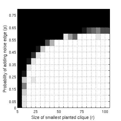
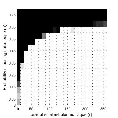
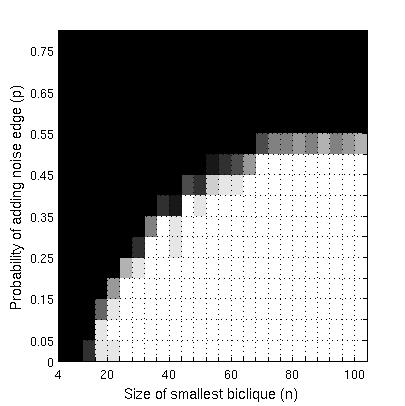
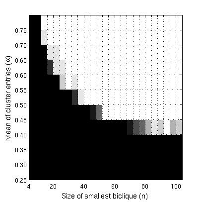
For and and a variety of choices of , the following procedure was repeated times. We first partition the indices into subsets of size at least . We then generate a random symmetric matrix according to the planted cluster model with respect to and one of two sets of probability distributions. In the first, is a Bernoulli random variable with probability of success if both belong to for some and is a Bernoulli random variable with probability of success otherwise, for some fixed probability . In the second, each is Gaussian with , for some if and belong to the same block, and otherwise. For each choice of and , the ADMM procedure described above is called to approximately solve (2.5). In each experiment, the algorithm is terminated if the stopping criteria is achieved with error tolerance or after iterations, and the subproblem (6.2) is solved to within error tolerance during each iteration. Let denote the optimal solution for (2.5) returned by the ADMM algorithm. We declare the block structure of to be successfully recovered if , where is the proposed solution constructed according to (2.6).
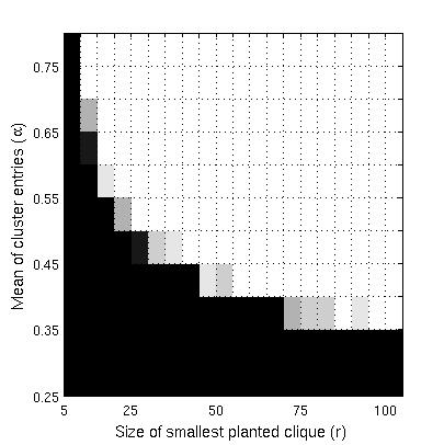
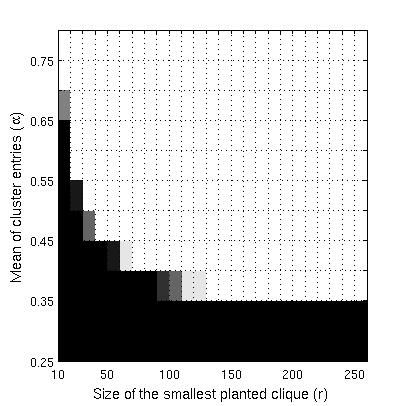
Figures 6.1 and 6.2 display the average number of successes for each choice of for sampled from the planted cluster model according to the Bernoulli and Gaussian distributions, respectively. The empirical performance of our heuristic appears to match that predicted by Theorem 2.1. For each choice of or , there is a sharp phase transition between zero and perfect recovery as increases past some threshhold. It should be noted that the recovery guarantees given by Theorem 2.1 appear to be conservative compared to those observed empirically; we have perfect recovery for values of smaller than the left-hand side of (2.8) for many trials. Moreover, generated according to the Gaussian model do not necessarily satisfy the assumption for .
We repeated the experiment for bipartite graphs drawn from the planted bicluster model. For , and various minimum bicluster sizes , we randomly sample weight matrices from the planted bicluster model according to some partition of into bicliques with left and right vertex sets of size at least and respectively. For each , we solve (3.5) using the ADMM algorithm described above and declare the block structure to be recovered if the returned optimal solution satisfies , where is the proposed solution constructed according to (3.6). We plot the number of successful recoveries for each and generating distribution in Figure 6.3. As before, the empirical behaviour of our heuristic reflects that predicted by Theorem 3.1, although there is some evidence that this theoretical recovery guarantee may be overly pessimistic.
7 Acknowledgements
This research was supported in part by the Institute for Mathematics and its Applications with funds provided by the National Science Foundation, and by a Postgraduate Scholarship from NSERC (Natural Science and Engineering Research Council of Canada). I am grateful to Stephen Vavasis, Henry Wolkowicz, Levent Tunçel, Shai Ben-David, Inderjit Dhillon, Ben Recht, and Ting Kei Pong for their helpful comments and suggestions. I am especially grateful to Ting Kei for his help implementing the ADMM algorithms used to perform the numerical trials. I would also like to thank Warren Schudy for suggesting some relevant references that were omitted in an earlier version. Finally, I thank the two anonymous reviewers, whose suggestions vastly improved the presentation and organization of this paper.
References
- [1] M. Ackerman and S. Ben-David. Clusterability: A theoretical study. Proceedings of AISTATS-09, JMLR: W&CP, 5:1–8, 2009.
- [2] D. Aloise, A. Deshpande, P. Hansen, and P. Popat. Np-hardness of euclidean sum-of-squares clustering. Machine Learning, 75(2):245–248, 2009.
- [3] B. Ames and S. Vavasis. Convex optimization for the planted k-disjoint-clique problem. Arxiv preprint arXiv:1008.2814, 2010.
- [4] B. Ames and S. Vavasis. Nuclear norm minimization for the planted clique and biclique problems. Mathematical Programming, 129(1):1–21, 2011.
- [5] S. Balakrishnan, M. Xu, A. Krishnamurthy, and A. Singh. Noise thresholds for spectral clustering. Advances in Neural Information Processing Systems, 25(3), 2011.
- [6] N. Bansal, A. Blum, and S. Chawla. Correlation clustering. Machine Learning, 56(1):89–113, 2004.
- [7] P. Berkhin. Survey of clustering data mining techniques. Grouping Multidimensional Data: Recent Advances in Clustering, pages 25–71, 2006.
- [8] E. Birgin, J. Martínez, and M. Raydan. Nonmonotone spectral projected gradient methods on convex sets. SIAM Journal on Optimization, 10(4):1196–1211, 2000.
- [9] S. Boyd, N. Parikh, E. Chu, B. Peleato, and J. Eckstein. Distributed optimization and statistical learning via the alternating direction method of multipliers. Foundations and Trends in Machine Learning, 3(1):1–122, 2011.
- [10] S. Boyd and L. Vandenberghe. Convex optimization. Cambridge University Press, Cambridge, UK, 2004.
- [11] S. Busygin, O. Prokopyev, and P. Pardalos. Biclustering in data mining. Computers & Operations Research, 35(9):2964–2987, 2008.
- [12] E. Candès and Y. Plan. Tight oracle bounds for low-rank matrix recovery from a minimal number of random measurements. Arxiv preprint arXiv:1001.0339, 2010.
- [13] E. Candès and B. Recht. Exact matrix completion via convex optimization. Foundations of Computational Mathematics, 9(6):717–772, 2009.
- [14] E. Candès, J. Romberg, and T. Tao. Stable signal recovery from incomplete and inaccurate measurements. Communications on Pure and Applied Mathematics, 59(8):1207–1223, 2006.
- [15] E. Candès and T. Tao. Decoding by linear programming. Information Theory, IEEE Transactions on, 51(12):4203–4215, 2005.
- [16] D. Donoho. Compressed sensing. Information Theory, IEEE Transactions on, 52(4):1289–1306, 2006.
- [17] Jonathan Eckstein and Dimitri P Bertsekas. On the douglas—rachford splitting method and the proximal point algorithm for maximal monotone operators. Mathematical Programming, 55(1-3):293–318, 1992.
- [18] N. Fan, N. Boyko, and P. Pardalos. Recent advances of data biclustering with application in computational neuroscience. Computational Neuroscience, pages 105–132, 2010.
- [19] N. Fan and P. Pardalos. Multi-way clustering and biclustering by the ratio cut and normalized cut in graphs. Journal of Combinatorial Optimization, pages 1–28, 2012.
- [20] C. Flynn and P. Perry. Consistent biclustering. Arxiv preprint arXiv:1206.6927, 2012.
- [21] Z. Füredi and J. Komlós. The eigenvalues of random symmetric matrices. Combinatorica, 1(3):233–241, 1981.
- [22] S. Geman. A limit theorem for the norm of random matrices. Ann. Probab., 8(2):252–261, 1980.
- [23] G. Golub and C. Van Loan. Matrix computations. Johns Hopkins University Press, 1996.
- [24] D. Gross. Recovering low-rank matrices from few coefficients in any basis. Information Theory, IEEE Transactions on, 57(3):1548–1566, 2011.
- [25] W. Hoeffding. Probability inequalities for sums of bounded random variables. J. American Statistical Assoc., 58:13–30, 1962.
- [26] A. Jalali, Y. Chen, S. Sanghavi, and H. Xu. Clustering partially observed graphs via convex optimization. Arxiv preprint arXiv:1104.4803, 2011.
- [27] R. Kannan, S. Vempala, and A. Vetta. On clusterings: Good, bad and spectral. Journal of the ACM (JACM), 51(3):497–515, 2004.
- [28] M. Kolar, S. Balakrishnan, A. Rinaldo, and A. Singh. Minimax localization of structural information in large noisy matrices. Advances in Neural Information Processing Systems, 2011.
- [29] Z. Lu and Y. Zhang. Penalty decomposition methods for rank minimization. Technical report, Technical Report. Department of Mathematics, Simon Fraser University. Arxiv preprint, 2010.
- [30] C. Mathieu and W. Schudy. Correlation clustering with noisy input. In Proceedings of the Twenty-First Annual ACM-SIAM Symposium on Discrete Algorithms, pages 712–728. Society for Industrial and Applied Mathematics, 2010.
- [31] A. Ng, M. Jordan, and Y. Weiss. On spectral clustering: Analysis and an algorithm. Advances in neural information processing systems, 2:849–856, 2002.
- [32] R. Ostrovsky, Y. Rabani, L. Schulman, and C. Swamy. The effectiveness of Lloyd-type methods for the k-means problem. In Proceedings of 47st Annual IEEE Symposium on the Foundations of Computer Science, 2006.
- [33] S. Oymak and B. Hassibi. Finding dense clusters via “low rank + sparse” decomposition. Arxiv preprint arXiv:1104.5186, 2011.
- [34] S. Oymak, K. Mohan, M. Fazel, and B. Hassibi. A simplified approach to recovery conditions for low rank matrices. In Information Theory Proceedings (ISIT), 2011 IEEE International Symposium on, pages 2318–2322. IEEE, 2011.
- [35] J. Peng and Y. Wei. Approximating k-means-type clustering via semidefinite programming. SIAM Journal on Optimization, 18(1):186–205, 2007.
- [36] B. Recht. A simpler approach to matrix completion. Journal of Machine Learning Research, 12:3413–3430, 2011.
- [37] B. Recht, M. Fazel, and P. Parrilo. Guaranteed Minimum-Rank Solutions of Linear Matrix Equations via Nuclear Norm Minimization. SIAM Review, 52(471), 2010.
- [38] B. Recht, W. Xu, and B. Hassibi. Null space conditions and thresholds for rank minimization. Mathematical Programming, pages 1–28, 2010.
- [39] R.T. Rockafellar. Convex analysis. Princeton Univ Press, 1997.
- [40] K. Rohe, S. Chatterjee, and B. Yu. Spectral clustering and the high-dimensional stochastic blockmodel. The Annals of Statistics, 39(4):1878–1915, 2011.
- [41] K. Rohe and B. Yu. Co-clustering for directed graphs; the stochastic co-blockmodel and a spectral algorithm. Arxiv preprint arXiv:1204.2296, 2012.
- [42] R. Shamir and D. Tsur. Improved algorithms for the random cluster graph model. Algorithm Theory—SWAT 2002, pages 230–239, 2002.
- [43] V. Singh, L. Mukherjee, J. Peng, and J. Xu. Ensemble clustering using semidefinite programming with applications. Machine learning, 79(1):177–200, 2010.
- [44] L. Tunçel. Polyhedral and semidefinite programming methods in combinatorial optimization. American Mathematical Society, 2010.
- [45] E. Van Den Berg and M. Friedlander. Probing the pareto frontier for basis pursuit solutions. SIAM Journal on Scientific Computing, 31(2):890–912, 2008.