Nonlinear modes in finite-dimensional ${\cal PT}$-symmetric systems

Abstract

By rearrangements of waveguide arrays with gain and losses one can simulate transformations among parity-time (${\cal PT}$-) symmetric systems not affecting their pure real linear spectra. Subject to such transformations, however, the nonlinear properties of the systems undergo significant changes. On an example of an array of four waveguides described by the discrete nonlinear Schrödinger equation with dissipation and gain, we show that the equivalence of the underlying linear spectra implies similarity of neither structure nor stability of the nonlinear modes in the arrays. Even the existence of one-parametric families of nonlinear modes is not guaranteed by the ${\cal PT}$ symmetry of a newly obtained system. Neither the stability is directly related to the ${\cal PT}$ symmetry: stable nonlinear modes exist even when the spectrum of the linear array is not purely real. We use graph representation of ${\cal PT}$-symmetric networks allowing for simple illustration of linearly equivalent networks and indicating on their possible experimental design.

The effect of dissipation or gain on dynamics of a physical system is a fundamental issue either in classical or in quantum theories. Optics is one of the areas where the respective models appear naturally and are explored already for many years in contexts of different kinds of dissipative solitons diss_solit . One of a number of widely used, fundamental and simple models is an array of waveguides in the presence of gain and losses waveguide . This model is described by the discrete nonlinear Schrödinger equation (DNLSE), which is fairly general. Its applications range from the so-called discrete optics disc_opt to biophysics biophysics and the meanfield theory of Bose-Einstein condensate BEC (for a broad range of applications of DNLSE see also general ).

Recently, great interest in systems with dissipation and gain was triggered by the discovery of the so-called parity-time (${\cal PT}$) potentials, which in a definite range of parameters obey purely real spectrum Bender . Numerous linear physical systems for which ${\cal PT}$ symmetry is of great relevance have been proposed. Among them we mention non-Hermitian extension of quantum mechanics quantum , electromagnetic wave propagation in a planar waveguide filled with active media Muga , and beam propagation in optical lattices Markis . The phenomenon of ${\cal PT}$ symmetry breaking has been experimentally implemented in optics experiment , where the equations governing the system were earlier known as describing a unidirectional coupler, i.e. as a particular form of the DNLSE waveguide .

Nonlinear ${\cal PT}$-symmetric problems were first posed in the context of the quantum field theory accounting for cubic interactions Bender_nonlin and in guided wave theory Christodoulides1 . Being natural for optical applications, the nonlinear problems received particular attention in the context of existence of gap solitons Christodoulides1 and defect modes defect in ${\cal PT}$-symmetric lattices, as well as in context of the nonlinear ${\cal PT}$-symmetric couplers in stationary coupler_stat ; Kevr2011 and solitonic coupler_solit regimes. More generally, the nonlinearity enriches possible statements of the problem allowing for including the effects on nonlinear PT-nonlin , as well as both linear and nonlinear PT-lin-nonlin ${\cal PT}$-symmetric potentials.

It is known that by applying a similarity transformation to a given linear ${\cal PT}$-symmetric system, a new system with real spectrum can be constructed. Thus in Darboux new potentials (not necessarily ${\cal PT}$-symmetric) with real spectra were constructed using the Darboux transformation, while in Mostaf2003 pseudo-Hermitian operators were introduced and unitary equivalence of ${\cal PT}$-symmetric and Hermitian operators was established. It turns out, however, that possible mutual reductions of Hermitian, ${\cal PT}$-symmetric, and pseudo-Hermitian linear operators leaving the spectrum pure real, may introduce dramatic changes in the properties of the respective nonlinear systems. The analysis of such changes is the main goal of the present Letter.

More specifically, we show that ${\cal PT}$-symmetric systems obeying the same linear spectrum may either have one-parametric families of nonlinear modes or have not. If the families exist, stability of the modes is essentially different for different systems, still having the same linear spectrum. Moreover, stable nonlinear modes may exist beyond the ${\cal PT}$ symmetry breaking. For a discrete system consisting of four waveguides we find that breaking of ${\cal PT}$ symmetry can occur in two different ways: the linear spectrum acquires either two complex and two real eigenvalues, or all four eigenvalues become complex. Finally, we represent each underlying linear system by a graph, allowing one to catalog different linearly equivalent ${\cal PT}$-symmetric systems.

We consider an array of $N$ waveguides (sites) and denote the field in the $n$th waveguide by $q_{n}(z)$, where $z$ is the propagation distance. If each waveguide have dissipation or gain described by $\gamma_{n}$, positive or negative, respectively, then the field propagation is governed by the DNLSE

$$i\dot{q}_{n}=-\sum_{m=1}^{N}K_{nm}q_{m}-|q_{n}|^{2}q_{n}-i\gamma_{n}q_{n},$$ (1)

where $\dot{q}_{n}=dq(z)/dz$. Here we admit the existence of non-local coupling among the waveguides, which is described by the coefficients $K_{nm}=K_{mn}={K}^{*}_{nm}$ which will be treated as entries of the real symmetric matrix ${\bf K}$: ${\bf K}={\bf K}^{\dagger}$, where ${\bf K}^{\dagger}$ is the Hermitian conjugate matrix. It is convenient to introduce diagonal matrices ${\bf G}=\mbox{diag}(\gamma_{1},...,\gamma_{N})$ and ${\bf F}({\bf q})=\mbox{diag}(|q_{1}|^{2},|q_{2}|^{2},\ldots,|q_{N}|^{2})$, which describe the dissipation and the nonlinear part of the system, respectively. Then the system (1) can be rewritten in the form

$$i\dot{\bf q}=-[{\bf H}+{\bf F}(\bf q)]{\bf q},\quad\mbox{ ${\bf H}={\bf K}+i{\bf G}$}.$$ (2)

We search stationary nonlinear modes in the form ${{\bf q}}(z)=e^{i{b}z}{{\bf w}}$, where $b$ is the propagation constant, and ${\bf w}=(w_{1},w_{2},\ldots,w_{N})^{T}$ solves the stationary DNLSE

$$b{\bf w}=[{\bf H}+{\bf F}({\bf w})]{\bf w}.$$ (3)

Requiring the spectrum of the linear problem $b{\bf w}={\bf H}{\bf w}$ to be real, which is necessary for all linear modes to be propagating, we impose the constraint $\sum_{n=1}^{N}\gamma_{n}=0$.

The matrix ${\bf H}$ is ${\cal PT}$-symmetric if it commutes with a ${\cal PT}$ operator: $[{\cal PT},{\bf H}]=0$. Hereafter ${\cal P}$ is an orthogonal symmetric (and therefore Hermitian) matrix, and ${\cal T}$ is element-wise complex conjugation: ${\cal T}{\bf q}={\bf q}^{*}$. Using that ${\bf H}^{\dagger}={\cal T}{\bf H}{\cal T}={\cal P}{\bf H}{\cal P}$, we observe that the linear system $i\dot{\bf q}=-{\bf H}{\bf q}$ admits an integral of motion (see also Znojil ) $Q=\frac{1}{N}\langle{\cal P}{\bf q},{\bf q}\rangle$, where the inner product is defined as $\langle{\bf u},{\bf v}\rangle=\sum_{n=1}^{N}v_{n}^{*}u_{n}$.

Now we can specify the problem at hand: we consider the existence and stability of nonlinear modes of ${\cal PT}$-symmetric lattices whose linear parts are related to each other by similarity transformations, all having the nonlinearity of the on-site type. Such a statement is natural for arrays of optical waveguides, since linear links among them can be arranged by assembling waveguides in different geometries, while the dissipation/gain and the nonlinearity are the characteristics of each particular waveguide, which can be routinely controlled (see also Fig. 3). One of our main findings is that linearly equivalent ${\cal PT}$-symmetric lattices result in qualitatively different properties of their nonlinear extensions.

${\cal PT}$-symmetric “quadrimer”–

Since the gain and dissipation must compensate each other, the simplest models allowing for nontrivial distribution of the dissipation have three or four waveguides. Below we concentrate on a quadrimer, respectively setting $N=4$. We start by revisiting recently considered in Kevr2011 system with the next-neighbor interactions: $K_{nm}=\delta_{|n-m|,1}$. The corresponding matrix, which we denote as ${\bf H}_{0}$, is ${\cal PT}$-symmetric with respect to ${{\cal P}}_{0}=\left(\begin{array}[]{cc}{\bf 0}&\sigma_{1}\\ \sigma_{1}&{\bf 0}\end{array}\right)$ (hereafter $\sigma_{1,2,3}$ are the Pauli matrices and ${\bf 0}$ is the $2\times 2$ zero matrix). Depending on particular values of $\gamma_{1,2}$, three different situations are possible: (i) unbroken or exact ${\cal PT}$ symmetry, when all the eigenvalues $\tilde{b}_{n}$, $n=1,...,4$, of ${\bf H}_{0}$ are real; (ii) broken ${\cal PT}$ symmetry with two real and two complex conjugated eigenvalues (notice that this is possible only if $\gamma_{1}\neq\gamma_{2}$); (iii) broken ${\cal PT}$ symmetry with all $\tilde{b}_{n}$ complex. Thus, the “phase space” $(\gamma_{1},\gamma_{2})$ can be divided into three domains as it is shown in the phase diagram (PD) of Fig. 1. A feature of the phase diagram is the existence of the triple points $T_{j}$, $j=1,\ldots,4$, where the three domains touch. The triple points correspond to values $\gamma_{1,2}$ for which $\tilde{b}_{n}=0$ for each $n=1,...,4$. Depending on how $\gamma_{1,2}$ change in vicinity of $T_{j}$, either the ${\cal PT}$-symmetric phase or one of the ${\cal PT}$ symmetry broken phases arise.

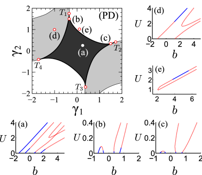
Figure 1: “Phase diagram” (PD) for the linear quadrimer ${\bf H}_{0}$. The dark-grey diamond-shaped domain corresponds to unbroken ${\cal PT}$ symmetry; in the light-gray domains there are two real and two complex eigenvalues. In the white domains all eigenvalues are complex. In panels (a)–(e), corresponding to the points (a)–(e) in the panel (PD), we show families of nonlinear modes for: (a) $\gamma_{1,2}=0.25$; (b) $\gamma_{1}\approx-0.37$, $\gamma_{2}\approx 1.49$; (c) $\gamma_{1}\approx 1.49$, $\gamma_{2}\approx 0.36$; (d) $\gamma_{1,2}=\mp 1$; (e) $\gamma_{1}=0.1$, $\gamma_{2}=0.95$. Stable (unstable) modes are shown by solid blue (dashed red) lines.

Figure 2: Families of nonlinear modes of the Hermitian quadrimers, whose linear parts are described by ${\bf H}_{H}$, chosen to have the same linear eigenvalues $\tilde{b}_{n}$ as the corresponding ${\cal PT}$-symmetric quadrimers ${\bf H}_{0}$ illustrated in the panel (a), (b), and (c) of Fig. 1.

If ${\bf H}_{0}$ is exactly ${\cal PT}$-symmetric, then its linear eigenstates $\tilde{\bf w}$ are simultaneously the eigenstates of the corresponding ${\cal PT}$ operator, i.e. ${\cal P}_{0}{\cal T}\tilde{{\bf w}}=\tilde{{\bf w}}$ (up to irrelevant phase shift). It is natural to look for nonlinear modes that possess the same property: ${\cal P}_{0}{\cal T}{\bf w}={\bf w}$. Therefore we require $w_{1}=w_{4}^{*}$, $w_{2}=w_{3}^{*}$, which reduces Eq. (3) to

$$bw_{1} = w_{2}+|w_{1}|^{2}w_{1}+i\gamma_{1}w_{1},$$ (4a)

$$bw_{2} = (w_{1}+w_{2}^{*})+|w_{2}|^{2}w_{2}+i\gamma_{2}w_{2}.$$ (4b)

We represent $w_{1}=W_{1}e^{i\Phi}$, where $W_{1}$ and $\Phi$ are real. Then Eq. (4a) gives $w_{2}=W_{2}e^{i\Phi}$, where $W_{2}={W_{1}}(b-W_{1}^{2}-i\gamma_{1})$ is complex, and from Eq. (4b) we obtain $e^{-2i\phi}=f(W_{1})$, where $f(W_{1})={\left(bW_{2}-W_{1}-|W_{2}|^{2}W_{2}-i\gamma_{2}W_{2}\right)}/{W_{2}^{*}}$. If a root of the equation $|f(W_{1})|^{2}=1$ is found, then $w_{1}$ and $w_{2}$ can be readily obtained. Thus nonlinear modes of the quadrimer correspond to the roots of a single equation $|f(W_{1})|^{2}=1$ with respect to one real unknown $W_{1}$. It is a purely technical matter to reduce the latter equation to: $P_{8}(W_{1}^{2})=0$, where $P_{8}(\xi)$ is an eighth-degree polynomial with real coefficients. Each positive root of $P_{8}(\xi)$ corresponds to a nonlinear mode of the quadrimer. Since the roots depend continuously on $b$, the nonlinear modes constitute continuous families for fixed parameters of the system com3 . As it is customary, such families can be represented on the plane $(U,b)$ where $U=\frac{1}{4}\sum_{n=1}^{4}|w_{n}|^{2}$ is the total energy flow in the array. Panels (a)–(e) of Fig. 1 illustrate typical examples of the families, as well as linear stability of the modes. When $\gamma_{1,2}$ belong to the domain of unbroken ${\cal PT}$ symmetry [see Fig. 1 (a)], one observes four families branching off from the linear limit, i.e. from the points $b=\tilde{b}_{n}$, $U=0$. In Fig. 1 (a) there also exist families that can not be continued from the linear limit. In panels (b) and (c) we also address the points that belong to the domain of unbroken ${\cal PT}$ symmetry but are situated closely to the triple points $T_{1,2}$. In these panels one observes that after the bifurcation from the linear limit, all four families rapidly lose stability and two of them cease to exist if $U$ is sufficiently large. Comparing panel (a) with panels (b) and (c), we conclude that increase of $\gamma_{1,2}$, i.e. approaching the ${\cal PT}$ symmetry breaking boundary, is unfavorable for existence and stability of the modes. However, the most surprising fact, is that stable nonlinear modes can be found in the domains of broken ${\cal PT}$ symmetry. Both in panel (d), which addresses the case when the spectrum consists of two real and two complex eigenvalues, and in panel (e), i.e. when all the eigenvalues are complex, one can find stable modes.

Hermitian quadrimer–

If ${\bf H}_{0}$ is exactly ${\cal PT}$-symmetric, then there exists a unitary matrix ${\bf R}$, which transforms ${\bf H}_{0}$ to a Hermitian matrix ${\bf H}_{H}$ Mostaf2003 : ${\bf R}{{\bf H}_{0}}{\bf R}^{-1}={\bf H}_{H}={\bf H}_{H}^{\dagger}$. This means that in the linear limit the modes in the array with gain and losses described by ${\bf H}_{0}$ have the same propagation constants as the modes in the array without gain and losses, which is described by ${\bf H}_{H}$. Hence, for any $\gamma_{1,2}$ lying in the domain of unbroken ${\cal PT}$-symmetry of ${\bf H}_{0}$, one can introduce a new DNLSE $i\dot{{\bf q}}=-[{\bf H}_{H}+{\bf F}({\bf q})]{\bf q}$ [c.f. (2)]. Following Mostaf2003 , one can find ${\bf H}_{H}$ explicitly and observe that all its nonzero elements are real and given by ${\bf H}_{H,{12}}={\bf H}_{H,{21}}=h_{1}$, ${\bf H}_{H,{14}}={\bf H}_{H,{41}}=h_{2}$, ${\bf H}_{H,{23}}={\bf H}_{H,{32}}=h_{3}$, with $h_{j}$ being dependent on $\gamma_{1,2}$. By construction, the matrix ${\bf H}_{H}$ has the same eigenvalues as ${\bf H}_{0}$ for the given $\gamma_{1,2}$.

Unlike in the ${\cal PT}$-symmetric case, the modes of the nonlinear system with linear part described by ${\bf H}_{H}$ can be searched as real-valued and either even or odd, i.e. solving the system $bw_{1}=h_{1}w_{2}\pm h_{2}w_{1}+w_{1}^{3}$, $bw_{2}=h_{1}w_{1}\pm h_{3}w_{2}+w_{2}^{3}$, where “$+$” (“$-$”) stays for even (odd) modes. This system is equivalent to a fourth-degree polynomial equation with respect to $w_{1}^{2}$. Families of even and odd nonlinear modes of the Hermitian quadrimer are illustrated in Fig. 2. Comparing Fig. 1 and Fig. 2, we observe that even if the matrices ${\bf H}_{0}$ and ${\bf H}_{H}$ have the same eigenvalues, the respective nonlinear systems show considerable differences in the properties of modes. The most visible differences are: (i) for the Hermitian system, the families bifurcating from the linear limit never close forming a saddle-node bifurcation [c.f. panels (b) and (c) in Fig. 1 and Fig. 2]; (ii) the leftmost family of the Hermitian system is always stable; (iii) in general, stable nonlinear modes of Eq. (2) with ${\bf H}_{0}$ and ${\bf H}_{H}$ correspond to different values of the propagation constant $b$.

“Generalized” quadrimer–

Being of the dissipative nature, the considered above ${\cal PT}$-symmetric quadrimer with linear part described by ${\bf H}_{0}$ possesses a property, usually typical for conservative systems – for the given parameters of the system (inter-site interactions ${\bf K}$ and dissipation $\gamma_{1,2}$) its nonlinear modes constitute continuous families rather than appear as isolated attractors. This peculiarity of nonlinear ${\cal PT}$-symmetric systems was reported in several studies Christodoulides1 ; Kevr2011 ; PT-nonlin ; PT-lin-nonlin . Here we argue that existence of the continuous families of nonlinear modes is not a typical property of ${\cal PT}$-symmetric systems. Specifically, the nonlinear ${\cal PT}$-symmetric systems that admit the families of the modes appear as “isolated points” in a continuous set of generic ${\cal PT}$-symmetric systems.

To this end we focus on the particular case $\gamma_{1}=\gamma_{2}=\gamma$, i.e. ${\bf G}=\mbox{diag}(\gamma,\gamma,-\gamma,-\gamma)$, and introduce an one-parametric family of matrices ${\bf H}_{0}(\beta)={\bf K}_{0}(\beta)+i{\bf G}$ with

$${\bf K}_{0}(\beta)=\left(\begin{array}[]{cccc}0&1&0&0\\ 1&0&\cos\beta&-\sin\beta\\ 0&\cos\beta&\sin 2\beta&\cos 2\beta\\ 0&-\sin\beta&\cos 2\beta&-\sin 2\beta\end{array}\right),$$

and real parameter $\beta$. One can ensure that ${\bf H}_{0}(\beta)$ is ${\cal PT}$-symmetric with respect to ${{\cal P}}_{0}(\beta)=\left(\begin{array}[]{cc}{\bf 0}&\rho(\beta)\\ \rho(\beta)&{\bf 0}\end{array}\right)$, where $\rho(\beta)=\cos\beta\ \sigma_{1}+\sin\beta\ \sigma_{3}$. For $\beta=0$ the matrix ${\bf K}_{0}(0)$ includes only the next-neighbor interactions, i.e. ${\bf H}_{0}(0)$ is merely the linear part of the ${\cal PT}$-symmetric quadrimer studied above (with $\gamma_{1}=\gamma_{2}$). Definition of ${\bf H}_{0}(\beta)$ guarantees that its eigenvalues do not depend on $\beta$. But the eigenvectors of ${\bf H}_{0}(\beta)$ do depend on $\beta$.

Next, using ${\bf M}=\left(\begin{array}[]{cc}\mu&{\bf 0}\\ {\bf 0}&\mu\end{array}\right)$, where $\mu=\sigma_{3}+i\sigma_{2}$, one can generate a new matrix ${{\bf H}}_{1}(\beta)={\bf M}{\bf H}_{0}(\beta){\bf M}^{-1}$, where ${{\bf H}}_{1}(\beta)={\bf K}_{1}(\beta)+i{\bf G}$,

$${\bf K}_{1}(\beta)=\left(\begin{array}[]{cccc}1&0&-k_{-}&k_{+}\\ 0&-1&k_{-}&-k_{+}\\ -k_{-}&k_{-}&\cos 2\beta&\sin 2\beta\\ k_{+}&-k_{+}&\sin 2\beta&-\cos 2\beta\end{array}\right),$$

and $k_{\pm}=\frac{\sqrt{2}}{2}\sin(\beta\pm\frac{\pi}{4})$. Then ${\bf H}_{1}(\beta)$ is ${\cal PT}$-symmetric with respect to ${\cal P}_{1}(\beta)={\bf M}{\cal P}_{0}(\beta){\bf M}^{-1}$. Notice that the transformation ${\bf M}$ does not affect the dissipative component $i{\bf G}$, which is the same both for ${\bf H}_{0}(\beta)$ and ${\bf H}_{1}(\beta)$. Obviously, the eigenvalues of the matrix ${\bf H}_{1}(\beta)$ are the same as for ${\bf H}_{0}(\beta)$ and also do not depend on $\beta$.

To give better physical insight into the systems ${\bf H}_{0,1}(\beta)$, in Fig. 3 we introduce their weighted graph representation. The vertexes of graphs correspond to the sites $q_{n}$ while the edges (lines) represent inter-site coupling having weights equal to the values of the respective matrix elements: e.g. a line between the vertexes $q_{1}$ and $q_{2}$ corresponds to the elements $K_{1,2}=K_{2,1}$ of the matrix ${\bf K}$. Each vertex is supplied by the sign “$+$” or “$-$” corresponding to gain and dissipation. We notice that the loop edges, which describe the on-site interactions $K_{n,n}$, are not shown as being not relevant for the present consideration.

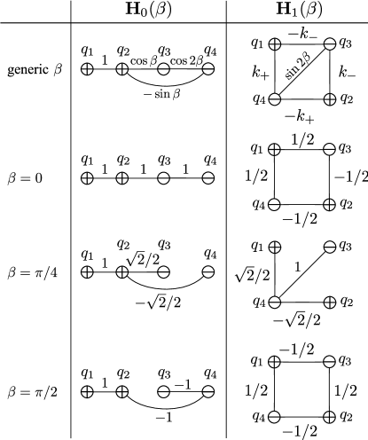
Figure 3: Graph representation of the systems ${\bf H}_{0,1}(\beta)$ for generic and particular values of $\beta$. In terms of the optical applications, the circles with “$+$” [or “$-$”] represent waveguides with gain [or losses], while the lines indicate the directions, along which the coupling of the field has to be arranged.

The graph representation can be viewed also as indication on how one could place and connect the waveguides in an experiment in order to obtain the desirable ${\cal PT}$-symmeric quadrimer. It is worth noting that, say the bottom graph in left column [i.e. ${\bf H}_{0}(\pi/2)$] can be reshaped into the line distribution of the waveguides similar to the graph ${\bf H}_{0}(0)$.

Existence of nonlinear modes–

Turning to nonlinear properties of the arrays, whose linear links are described by ${\bf H}_{0,1}(\beta)$, let us suppose that the $n$th eigenstate of the underlying linear problem $b{\bf w}={\bf H}_{0,1}(\beta){\bf w}$ gives rise to a family of nonlinear modes. Then in the vicinity of the bifurcation point the nonlinear modes can be described using the expansion ${\bf w}=\varepsilon\tilde{\bf w}_{n}+o(\varepsilon)$, and $b=\tilde{b}_{n}+\varepsilon^{2}b_{n}^{(2)}+o(\varepsilon^{2})$, where $\varepsilon$ is a small parameter, $\tilde{b}_{n}$ and $\tilde{\bf w}_{n}$ are the eigenvalue and the corresponding eigenvector of ${\bf H}_{0}(\beta)$ [or ${\bf H}_{1}(\beta)$]. The coefficient $b_{n}^{(2)}$ can be readily found: $b_{n}^{(2)}={\langle{\bf F}(\tilde{\bf w}_{n})\tilde{\bf w}_{n},\tilde{\bf w}_{n}^{*}\rangle}/{\langle\tilde{\bf w}_{n},\tilde{\bf w}_{n}^{*}\rangle}$. This means that the bifurcation of nonlinear modes is possible only if $\textrm{Im}\,b_{n}^{(2)}=0$ for all $n$ (we may conjecture that this condition is also sufficient for existence of the modes, what was observed in all our numerical simulations). The coefficient $b_{n}^{(2)}$ is easily computable. In Fig. 4 (left panel) $\textrm{Im}\,b_{n}^{(2)}$ is plotted for ${\bf H}_{0}(\beta)$. Only at $\beta=\beta_{k}=\pi k/2$ the coefficient $b_{n}^{(2)}$ becomes real for all $n$ and the system ${\bf H}_{0}(\beta)$ admits continuous families of nonlinear modes, while for all other $\beta$ nonlinear modes bifurcating from the linear limit were not found.

To understand peculiarity of the values $\beta_{k}$ we notice that relation ${\cal PT}\tilde{\bf w}_{n}=\tilde{\bf w}_{n}$ ensures that the denominator in the formula for $b_{n}^{(2)}$ is real for any $\beta$: $\langle\tilde{\bf w}_{n},\tilde{\bf w}_{n}^{*}\rangle=\langle{\cal PT}\tilde{\bf w}_{n},{\cal T}\tilde{\bf w}_{n}\rangle=\langle{\cal T}\tilde{\bf w}_{n},{\cal PT}\tilde{\bf w}_{n}\rangle=\langle\tilde{\bf w}_{n}^{*},\tilde{\bf w}_{n}\rangle$. Meanwhile $\langle{\bf F}(\tilde{\bf w}_{n})\tilde{\bf w}_{n},\tilde{\bf w}_{n}^{*}\rangle$ can have nonzero imaginary part. Then the reality of the coefficient $b_{n}^{(2)}$ is ensured by an additional constraint ${\cal PT}({\bf F}(\tilde{\bf w}_{n})\tilde{\bf w}_{n})={\bf F}(\tilde{\bf w}_{n})\tilde{\bf w}_{n}$, which is satisfied only for $\beta=\beta_{k}$.

For the system ${\bf H}_{1}(\beta)$ the situation is similar – the families of nonlinear modes exist only for $\beta=\pi k/2$ where $\textrm{Im}\,b_{n}^{(2)}=0$ for all $n$. In the right panel of Fig. 4 we show families of nonlinear modes of the array whose linear part is described by ${\bf H}_{1}(0)$ with $\gamma=0.25$. Comparing the latter panel with Fig. 1 (a) (which also corresponds to $\gamma_{1,2}=0.25$), we again notice that, whereas the corresponding arrays have the same eigenvalues in the linear limit, nonlinear modes of those arrays have essentially different properties.

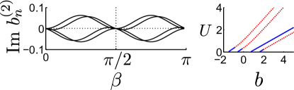
Figure 4: $\textrm{Im}\,b_{n}^{(2)}$ ($n=1,...,4$) vs $\beta$ for ${\bf H}_{0}(\beta)$ (left panel) and the families of modes of ${\bf H}_{1}(0)$ for $\gamma=0.25$ (right panel).

To conclude, we have considered nonlinear properties of different ${\cal PT}$-symmetric lattices (discrete nonlinear Schrödinger equations with gain and dissipation), whose linear parts are related by similarity transformations preserving the spectrum. Such systems describe, in particular, arrays of optical waveguides with either gain or losses, which are properly arranged in the space. Alternatively, a physical realization of the described phenomenon is possible in arrays of Bose-Einstein condensates loaded in multi-well potentials, provided the atoms are eliminated from given wells and are condensed in the other wells, simulating in this way losses and gain.

On the case example of a ${\cal PT}$-symmetric quadrimer we have shown that the spectral equivalence of the underlying linear systems implies neither similarity of the nonlinear modes nor their stability properties. We have found that the existence of one-parametric families of nonlinear modes is not guaranteed by the ${\cal PT}$ symmetry, and appears as a peculiarity of a system rather than a general property. It was also found that the stability of nonlinear modes is not directly related to the ${\cal PT}$ symmetry: stable nonlinear modes exist beyond the ${\cal PT}$ symmetry breaking threshold. If the system includes two different dissipative coefficients, then the “phase diagram” of the ${\cal PT}$-symmetric quadrimer allows for existence of “triple” points, where three different phases meet. Finally, we have shown that use of graph representation of ${\cal PT}$-symmetric networks gives straightforward indication on their possible experimental design in optics, and provides graphical illustration of linearly equivalent networks.

Authors acknowledge support of the FCT (Portugal) grants: SFRH/BPD/64835/2009, PTDC/FIS/112624/2009, and PEst-OE/FIS/UI0618/2011.

References

- (1) see e.g. Dissipative Solitons, eds. N. Akhmediev and A. Ankiewicz (Springer-Verlag, 2005); Focus Issue: Disspative Localized Structures in Exteded Systems, Chaos 17, (2007).
- (2) Y. Chen, A. W. Snyder, and D. N. Pain, IEEE J. Quant. Electron. 28, 239 (1992).
- (3) F. Lederer, G. I. Stegeman, D. N. Christodoulides, G. Assanto, M. Segev, and Y. Silberberg, Phys. Rep. 463, 1 (2008).
- (4) A. Scott, Nonlinear Science. Emergence and Dynamics of Coherent Structures (Oxford, University Press, 1999).
- (5) P. G. Kevrekidis and Frantzeskakis, Mod. Phys. Lett. B 18, 173 (2004); V. A. Brazhnyi, V. V. Konotop, Mod. Phys. Lett. B 18, 627 (2004); O. Morsch and M. Oberthaler, Rev. Mod. Phys. 78, 179 (2006).
- (6) P. G. Kevrekidis, The Discrete Nonlinear Schr dinger Equation (Springer, Berlin Heidelberg 2009).
- (7) C. M. Bender and S. Boettcher, Phys. Rev. Lett. 80, 5243 (1998).
- (8) C. M. Bender, S. Boettcher, and P. N. Meisinger, J. Math. Phys. 40, 2201 (1999).
- (9) A. Ruschhaupt, F. Delgado, J. G. Muga, J. Phys. A: Math. Gen. 38, L171 (2005).
- (10) K. G. Makris, R. El-Ganainy, D. N. Christodoulides, and Z. H. Musslimani, Phys. Rev. Lett. 100, 103904 (2008); S. Klaiman, U. Günther, and N. Moiseyev, Phys. Rev. Lett. 101 080402 (2008).
- (11) C. E. Rüter, K. G. Makris, R. El-Ganainy, D. N. Christodoulides, M. Segev, and D. Kip, Nature Phys. 6 192 (2010).
- (12) C. M. Bender, D. C. Brody, and H. F. Jones, Phys. Rev. D 70, 025001 (2004).
- (13) Z. H. Musslimani, K. G. Makris, R. El-Ganainy, and D. N. Christodoulides Phys. Rev. Lett. 100, 030402, (2008).
- (14) Xing Zhu, Hong Wang, Li-Xian Zheng, Huagang Li, and Ying-Ji He, Opt. Lett. 36, 2680 (2011).
- (15) H. Ramezani, T. Kottos, R. El-Ganainy, and D. N. Christodoulides, Phys. Rev. A 82, 043803 (2010); A. A. Sukhorukov, Z. Xu, and Yu. S. Kivshar, Phys. Rev. A 82, 043818 (2010).
- (16) K. Li and P. G. Kevrekidis, Phys. Rev. E 83, 066608 (2011).
- (17) R. Driben and B. A. Malomed Opt. Lett. 36, 4323 (2011); F. Kh. Abdullaev, V. V. Konotop, M. Ögren, and M. P. Sørensen Opt. Lett. 36, 4566 (2011).
- (18) F. Kh. Abdullaev, Y. V. Kartashov, V. V. Konotop, and D. A. Zezyulin, Phys. Rev. A 83 041805(R), (2011); D. A. Zezyulin, Y. V. Kartashov, V. V. Konotop, Europhys. Lett. 96, 64003 (2011).
- (19) A. E. Miroshnichenko, B. A. Malomed, and Yu. S. Kivshar, Phys. Rev. A 84, 012123 (2011); Y. He, X. Zhu, D. Mihalache, J. Liu, and Z. Chen, Phys. Rev. A 85, 013831 (2012).
- (20) F. Cannata, G. Junker, and J. Trost, Phys. Lett. A 246, 219 (1998).
- (21) A. Mostafazadeh, J. Math. Phys. 43, 205 (2002); J. Phys. A: Math. Gen. 36, 7081 (2003).
- (22) B. Bagchi, C. Quesne, and M. Znojil, Mod. Phys. Lett. A 16, 2047 (2001).
- (23) The continuous family of solutions presented herein is an additional one to the solutions found in Kevr2011 for , which required that the parameters of the system are inter-related. These two types of solutions are complementary in the complete set of possible standing wave solutions in this special case of equal values of the quadrimer gain/loss parameters.