Abstract

In the present work we have searched the existence of the late time acceleration of the universe with string fluid as source of matter in Bianchi V space-time. To get the deterministic solution, we choose the scale factor as increasing function of time that yields a time dependent deceleration parameter, representing a model which generates a transition of universe from early decelerating phase to recent accelerating phase. The study reveals that strings dominate the early universe and eventually disappear from the universe for sufficiently large times i. e. at present epoch. The same is observed by current astronomical observations. The physical behaviour of universe has been discussed in detail.

Keywords :String, Bianchi-V space-time, deceleration parameter
PACS number: 98.80.Cq, 98.80.-k

1 Introduction

In recent years, Einstein’s theory of gravity has been subject of intense study for his success in explaining the observed accelerated expansion of late time universe. The substantial theoretical progress in string theory has brought forth a diverse new generation of cosmological models, some of which are subject to direct observational tests. The present day observations of universe indicate the existence of large scale network of strings in early universe (Kible, 1976, 1980). One key advance is the emergence of methods of moduli stabilization. Compactification of string theory from the total dimension D down to four dimensions introduces many gravitationally-coupled scalar fields moduli from the point of view of the four dimensional theory. Recently we have studied inhomogeneous string cosmological model formed by geometric string and use this model as a source of gravitational field (Pradhan et al. 2007; Yadav et al. 2009). We had two main reason to study the above mentioned model. First, as a test of consistency, for some particular field theories based on string models and second we point out the universe can be represented by a collection of extended galaxies. It is generally assumed that after the big bang, the universe may have undergone a series of phase transitions as its temperature cooled below some critical temperature as predicted by grand unified theories (Zel’dovich et al. 1975; Kibble 1976, 1980; Everett 1981; Vilenkin 1981). At the very early stage of evolution of universe, it is believed that during the phase transition, the symmetry of universe was broken spontaneously. That could have given rise to topologically-stable defects such as domain walls, strings and monopoles (Vilenkin 1981). Among all the three cosmological structures, only cosmic strings have excited the most interesting consequence (Vilenkin 1985), because it gives rise the density perturbations which leads to the formation of galaxies. The cosmic string are important in the early stage of evolution of the universe before the particle creation because cosmic strings are one dimensional topological defects associated with spontaneous symmetry breaking whose plausible production site is cosmological phase transition in the early universe only. Also the present day observations reveal that the cosmic strings are not responsible for either the CMB fluctuations or the observed clustering of galaxies (Pogosian et al. 2006; Pogosian et al. 2003). The gravitational effect of cosmic strings have been extensively discussed by Letelier (1979) who considered the massive string to be formed by geometric strings with particle attached along its extension. Later on Letelier (1983) used this idea in obtaining cosmological solution in Bianchi-I and Kantowski-Sachs space-time.

Recently, Pradhan and Amirhashchi (2011) have studied the law of variation of scale factor as increasing function of time in Bianchi-V space-time, which generates a time dependent deceleration parameter (DP). This law provides explicit form of scale factors governing the Bianchi-V universe and facilitates to describe the transition of universe from early decelerating phase to recent accelerating phase. Yadav et al. (2011) and Bali (2008) have obtained Bianchi-V string cosmological models in general relativity. The string cosmological models with the magnetic field are discussed by Chakraborty (1980), Tikekar and Patel (1992, 1994), Patel and Maharaj (1996). Singh and Singh (1999) investigated string cosmological model with magnetic field in the context of space-time with $G_{3}$ symmetry. Saha and Visineusu (2008) have studied string cosmological model in presence of magnetic flux and concluded that the presence of cosmic string does not allow the anisotropic universe to evolves into an isotropic one. Recently Yadav (2011) studied Bianchi-I string cosmological model with variable DP. The study of Bianchi-V cosmological model create more interest as these models contain isotropic special cases and permit arbitrary small anisotropy levels at some instant of cosmic time. This property makes them suitable as model of our universe. The homogeneous and isotropic FRW cosmological models which are used to describe standard cosmological models, are particular case of Bianchi-V universes, according to whether the constant curvature of physical three-space, t = constant, is negative.

In this paper we have established the existence of string cosmological model with time varying DP in Bianchi-V space-time unlike the other authors. The organization of the paper is as follows: The model and field equations are presented in section 2. Section 3 deals with solution of field equations. The physical and geometrical properties of model is presented in section 4. Finally the conclusions of the paper are presented in section 5.

2 Bianchi V model and the field equations

The line element for the spatially homogeneous and anisotropic Bianchi-V space-time is given by

$$ds^{2}=-dt^{2}+A^{2}dx^{2}+e^{2\alpha x}\left(B^{2}dy^{2}+C^{2}dz^{2}\right)$$ (1)

where $A(t)$, $B(t)$ and $C(t)$ are the scale factors in different spatial directions and $\alpha$ is a constant.

We define $a=(ABC)^{1/3}$ as the average scale factor of the space-time (1) so that the average Hubble’s parameter reads as

$$H=\frac{\dot{a}}{a}$$ (2)

where an over dot denotes derivative with respect to the cosmic time t.

The energy-momentum tensor $T^{i}_{j}$ for a cloud of massive strings and perfect fluid distribution is taken as

$$T^{i}_{j}=(\rho+p)v^{i}v_{j}+pg^{i}_{j}-\lambda x^{i}x_{j},$$ (3)

where $p$ is the isotropic pressure; $\rho$ is the proper energy density for a cloud strings with particles attached to them; $\lambda$ is the string tension density; $v^{i}=(0,0,0,1)$ is the four-velocity of the particles, and $x^{i}$ is a unit space-like vector representing the direction of string. The vectors $v^{i}$ and $x^{i}$ satisfy the conditions

$$v_{i}v^{i}=-x_{i}x^{i}=-1,\;\;v^{i}x_{i}=0.$$ (4)

Choosing $x^{i}$ parallel to $\partial/\partial x$, we have

$$x^{i}=(A^{-1},0,0,0).$$ (5)

If the particle density of the configuration is denoted by $\rho_{p}$, then

$$\rho=\rho_{p}+\lambda.$$ (6)

The Einstein’s field equations (in gravitational units $c=1$, $8\pi G=1$) read as

$$R_{j}^{i}-\frac{1}{2}g_{j}^{i}R=-T_{j}^{i}$$ (7)

The Einstein’s field equations (7) for the line-element (1) lead to the following system of equations

$$\frac{\ddot{B}}{B}+\frac{\ddot{C}}{C}+\frac{\dot{B}\dot{C}}{BC}-\frac{\alpha^{2}}{A^{2}}=-p+\lambda$$ (8)

$$\frac{\ddot{A}}{A}+\frac{\ddot{C}}{C}+\frac{\dot{A}\dot{C}}{AC}-\frac{\alpha^{2}}{A^{2}}=-p$$ (9)

$$\frac{\ddot{A}}{A}+\frac{\ddot{B}}{B}+\frac{\dot{A}\dot{B}}{AB}-\frac{\alpha^{2}}{A^{2}}=-p$$ (10)

$$\frac{\dot{A}\dot{B}}{AB}+\frac{\dot{A}\dot{C}}{AC}+\frac{\dot{B}\dot{C}}{BC}-\frac{3\alpha^{2}}{A^{2}}=\rho$$ (11)

$$\frac{2\dot{A}}{A}-\frac{\dot{B}}{B}-\frac{\dot{C}}{C}=0$$ (12)

The energy conservation equation $T^{i}_{j\;;j}=0$ leads to the following expression

$$\dot{\rho}+(\rho+p)\left(\frac{\dot{A}}{A}+\frac{\dot{B}}{B}+\frac{\dot{C}}{C}\right)-\lambda\frac{\dot{A}}{A}=0$$ (13)

which is a consequence of the field equations.

3 Solution of field equations

Integrating equation (12) and absorbing the constant of integration in $B$ or $C$, without loss of generality, we obtain

$$A^{2}=BC$$ (14)

Subtracting equation (9) from (10) and taking second integral, we get the following relation

$$\frac{B}{C}=d_{1}exp\left(x_{1}\int{\frac{dt}{ABC}}\right)$$ (15)

where $d_{1}$ and $x_{1}$ are the constant of integrations.
Equations (8)$-$(12) are five independent equations in six unknown $A$, $B$, $C$, $p$, $\rho$ and $\lambda$. For the complete determination of the system, we need one extra condition.
Following Pradhan and Amirhashchi (2011),we assume that

$$a=\left(t^{n}e^{t}\right)^{\frac{1}{m}}$$ (16)

where $m$ and $n$ are positive constants. It is important to note here that the ansatz for scale factor generalized the one proposed by Pradhan and Amirhashchi (2011) because for $m=2$, we obtain the same expression for $a$ as proposed by Pradhan and Amirhashchi (2011) to describe the dark energy model in Bianchi V space-time. However in this paper, we considered string fluid as source of matter.
Now the spatial volume $V$ of the model read as

$$V=a^{3}=\left(t^{n}e^{t}\right)^{\frac{3}{m}}$$ (17)

Equations (14), (16) and (17) lead to

$$A(t)=\left(t^{n}e^{t}\right)^{\frac{1}{m}}$$ (18)

Inserting (18) into (14) and (15), we get

$$B=\left(t^{n}e^{t}\right)^{\frac{1}{m}}\sqrt{d_{1}}exp\left(\frac{x_{1}}{2}\int{\frac{dt}{\left(t^{n}e^{t}\right)^{\frac{3}{m}}}}\right)$$ (19)

$$C=\frac{\left(t^{n}e^{t}\right)^{\frac{1}{m}}}{\sqrt{d_{1}}}exp\left(-\frac{x_{1}}{2}\int{\frac{dt}{\left(t^{n}e^{t}\right)^{\frac{3}{m}}}}\right)$$ (20)

4 Some physical and geometrical properties

The isotropic pressure $(p)$, proper energy density $(\rho)$, string tension density $(\lambda)$ and particle density $(\rho_{p})$ are given by

$$p=\alpha^{2}(t^{n}e^{t})^{-\frac{2}{m}}+\frac{x_{1}}{m}\left(\frac{n}{t}+1\right)(t^{n}e^{t})^{-\frac{3}{m}}-\left[\frac{1}{m}\left(\frac{n}{t}+1\right)+\frac{x_{1}}{2}(t^{n}e^{t})^{-\frac{3}{m}}\right]^{2}$$ (21)

$$\rho=\frac{3}{m^{2}}\left(\frac{n}{t}+1\right)^{2}-\frac{x_{1}^{2}}{4}(t^{n}e^{t})^{-\frac{6}{m}}-3\alpha^{2}(t^{n}e^{t})^{-\frac{2}{m}}$$ (22)

$$\lambda=\frac{x_{1}}{m}\left(\frac{n}{t}+1\right)(t^{n}e^{t})^{-\frac{3}{m}}+\frac{1}{m^{2}}\left(\frac{n}{t}+1\right)^{2}+\left[\frac{1}{m}\left(\frac{n}{t}+1\right)+\frac{x_{1}}{2}(t^{n}e^{t})^{-\frac{3}{m}}\right]^{2}-\frac{2n}{mt^{2}}-\frac{x_{1}^{2}}{4}(t^{n}e^{t})^{-\frac{6}{m}}$$ (23)

$$\rho_{p}=\frac{2}{m^{2}}\left(\frac{n}{t}+1\right)^{2}+\frac{2n}{mt^{2}}-\frac{x_{1}}{m}\left(\frac{n}{t}+1\right)(t^{n}e^{t})^{-\frac{3}{m}}-\left[\frac{1}{m}\left(\frac{n}{t}+1\right)+\frac{x_{1}}{2}(t^{n}e^{t})^{-\frac{3}{m}}\right]^{2}-3\alpha^{2}(t^{n}e^{t})^{-\frac{2}{m}}$$ (24)

The average Hubble’s parameter $(H)$, expansion scalar $(\theta)$, anisotropy parameter $(A_{m})$ and shear scalar $(\sigma)$ of the model are given by

$$H=\frac{1}{m}\left(\frac{n}{t}+1\right)$$ (25)

$$\theta=3H=\frac{3}{m}\left(\frac{n}{t}+1\right)$$ (26)

$$A_{m}=\frac{1}{9H^{2}}\left[\left(\frac{\dot{A}}{A}-\frac{\dot{B}}{B}\right)^{2}+\left(\frac{\dot{B}}{B}-\frac{\dot{C}}{C}\right)^{2}+\left(\frac{\dot{C}}{C}-\frac{\dot{A}}{A}\right)^{2}\right]=\frac{m^{2}x_{1}^{2}}{6\left(\frac{n}{t}+1\right)}(t^{n}e^{t})^{-\frac{6}{m}}$$ (27)

$$\sigma^{2}=\frac{3}{2}A_{m}H^{2}=\frac{x_{1}^{2}}{4(t^{n}e^{t})^{\frac{6}{m}}}$$ (28)

The value of DP $(q)$ is found to be

$$q=-1+\frac{mn}{(n+t)^{2}}$$ (29)

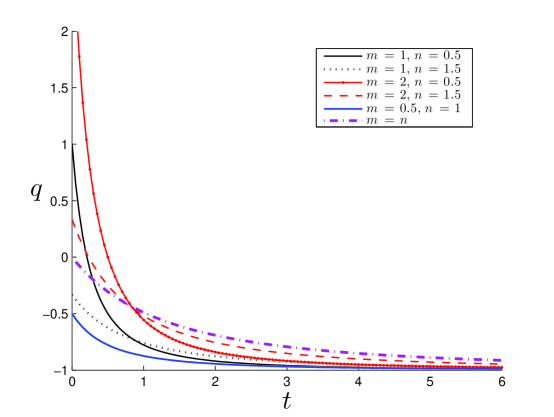
Figure 1: The plot of DP $(q)$ vs. time (t).

From Fig. 1, we see that the dynamics of DP $(q)$ depends on two free parameters $m$ and $n$. For $m=n$ (violet dash-dotted line), $m=1$ and $n=1.5$ (black dotted line) and $m=0.5,\;n=1$ (blue solid line), the universe is accelerating from its birth whereas for $m=1,\;n=0.5$ (solid black line), $m=2,\;n=0.5$ (solid red line with dot marker) and $m=2,\;n=1.5$ (dashed red line), it goes to transition from early decelerating phase to current accelerating phase. Since, we are looking for a model, describing the universe from early decelerating phase to current accelerating phase hence we choose $m=1$ and $n=0.5$ in the remaining discussions of the model as it is the most appropriate choice in our case.

From equation (29), it is clear that the DP $(q)$ is time dependent. Also, the transition redshift from deceleration expansion to accelerated expansion is about $0.5$. Now for a universe which was decelerating in past and accelerating at present time, DP must show signature flipping (Amendola 2003; Riess et al. 2001).

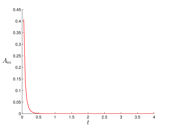
Figure 2: The plot of anisotropic parameter $A_{m}$ vs. time (t).

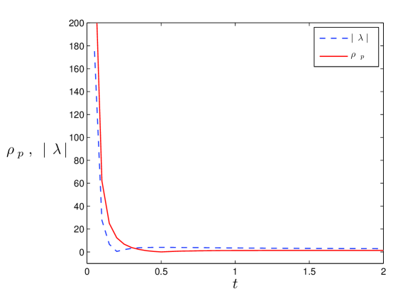
Figure 3: The particle density $(\rho_{p})$ and string tension density $(\lambda)$ vs. time (t).

It is observed that at $t=0$, the spatial volume vanishes and other parameters $H$, $\theta$ and $\sigma$ diverge. Hence the model starts with big bang singularity at $t=0$ and this singularity is point type because all directional scale factors vanish at initial moment. Figure 2 depicts the variation of anisotropic parameter $(A_{m})$ versus cosmic time. It is shown that $A_{m}$ decreases with time and tends to zero for sufficiently large times. Thus the anisotropic behaviour of universe dies out on later times and the observed isotropy of universe can be achieved in derived model at present epoch.

In this model the universe starts with finite values of proper energy density $(\rho)$, particle energy density $(\rho_{p})$ and string tension density $(\lambda)$ but with evolution of universe, $\rho$ and $\lambda$ becomes negligible for sufficiently long time (i. e. at present epoch). The large value of $\rho$ and $\arrowvert\lambda\arrowvert$ in the beginning suggest that string dominates the early universe but on later times, $\rho_{p}$ and $\arrowvert\lambda\arrowvert$ becomes negligible. Thus the strings disappear from the universe for larger times and hence it is not observable today. This behaviour of $\rho_{p}$ and $\arrowvert\lambda\arrowvert$ is shown in Figure 3. Since there is no direct evidence of strings in present day universe, we are in general, interested in constructing model of a universe that evolves purely from the era dominated by either geometric strings or massive strings and end up in a particle dominated era with or without remnants of strings. Therefore, the above model describes the evolution of the universe consistent with the present day observations.

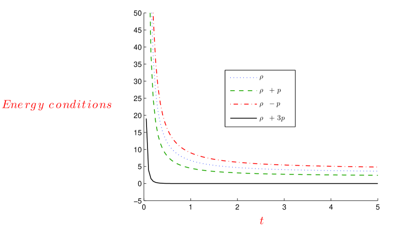
Figure 4: The energy conditions vs. time (t).

The left hand side of energy conditions have graphed in Figure 4. From Figure 4, we observe that
(i)  $\rho>0$  
(ii)  $\rho+p>0$  
(iii)  $\rho-p>0$

Therefore weak energy condition (WEC) as well as dominant energy condition (DEC) are satisfied in the derived model. It is also observed that $\rho+3p>0$ at initial moment and on later times $\rho+3p\leq 0$ which in turn imply that the strong energy condition (SEC) violates in derived model on later times. The violation of SEC gives a reverse gravitational effect. Due to this effect, the universe gets jerk and the transition from the earlier deceleration phase to the recent acceleration phase take place (Caldwell et al. 2006). Thus the model presented in this paper is turning out as a suitable model for describing the late time acceleration of the universe.

5 Concluding Remarks

In this paper, a spatially homogeneous and anisotropic Bianchi-V string model has been investigated for which the string fluid are rotation free but they do have expansion and shear. We observe that $V\rightarrow\infty$ and $\rho\rightarrow 0$ as $t\rightarrow\infty$  i. e. spatial volume $(V)$ increases with time and proper energy density $(\rho)$ decreases with time as expected. The main features of the derived model are as follows:

• The model is based on exact solution of Einstein’s field equations for the anisotropic Bianchi-V space-time filled with string fluid as source of matter.

• The dynamics of DP yields two different phases of the universe. Initially DP is evolving with positive sign that yields the decelerating phase of the universe whereas in later times, it is evolving with negative sign which describes the present phase of acceleration of the universe. Thus the derived model has transition of the universe from early decelerating phase to the current accelerating phase.

• In the present model, the WEC and DEC are satisfied which in turn imply that the derived models are physically realistic while the violation of SEC is in agreement with current astrophysical observations.

• The string tension density $(\lambda)$ start off with extremely large values and tends to zero for sufficiently large times in derived model. Thus the strings dominates the early universe and eventually disappear from the universe at later times (i. e. present epoch).

Finally, the solution presented here can be one of the potential candidates to describe the observed universe. Therefore physically viable Bianchi-V string cosmological model with singular origin has been obtained.

Acknowledgements

Author would like to thanks the anonymous referee for his valuable suggestions to improve the quality of this manuscript.

References

- [1] Amendola,L., 2003, Mon. Not. R. Astron. Soc., 342, 221
- [2] Bali, R., 2008, Electron. J. Theor. Phys., 5, 105
- [3] Caldwell, R. R., Knop, W., Parkar, L., Vanzell, D. A. T., 2006, Phys. Rev. D, 73, 023513
- [4] Chakraborty, S., 1980, Ind. J. Pure Appl. Phys., 29, 31
- [5] Everett., A. E., 1981, Phys. Rev., 24, 858
- [6] Kibble, T. W. B., 1976, J. Phys. A: Math. Gen., 9, 1387
- [7] Kibble, T. W. B., 1980, Phys. Rep., 67, 183
- [8] Latelier, P. S., 1979, Phys. Rev. D, 20, 1294
- [9] Latelier, P. S., 1983, Phys. Rev. D, 28, 2414
- [10] Pradhan, A., Amirhaschi, H., 2011, Mod. Phys. Lett. A, 26, 2261
- [11] Pradhan, A., Yadav, A. K., Singh, R .P. and Singh, V. K., 2007, Astrophys Space Sci., 312, 145
- [12] Patel, L. K., Maharaj, S. D., 1996 Pramana J. Phys., 47, 1
- [13] Pogosian, L., Wasserman, I. and Wyman, M., arXiv: astro-ph/0604141
- [14] Pogosian, L., Tye, S. H., Wasserman, I. and Wyman. M., 2003, Phys. Rev. D, 68, 023506
- [15] Riess, A. G., et al. 2001, Astrophys. J., 560, 49
- [16] Singh, G. P., Singh, T., 1999, Gen. Rel. Grav., 31, 371
- [17] Saha, B., Visinescu, M., 2008, Int. J. Theor. Phys., 49, 1411
- [18] Tikekar, R., Patel, L. K., 1992, Gen. Rel. Grav., 24, 397
- [19] Tikekar, R., Patel, L. K., 1994, Pramana J. Phys., 42, 483
- [20] Vilenkin, A., 1981, Phys. Rev. D, 24, 2082
- [21] Vilenkin, A., 1985, Phys. Rep., 121, 263
- [22] Yadav, A. K., Yadav, V. K. and Yadav, L., 2009, Int. J. Theor. Phys., 48, 568
- [23] Yadav, A. K., Yadav, V. K. and Yadav, L., 2011, Pramana J. Phys., 76, 681
- [24] Yadav, A. K., 2011, Anisotropic models of accelerating universe, LAP, 80 ; arXiv: 1009.3867 [gr-qc]
- [25] Zel’dovich, Ya. B., Kobzarev, Yu., and Okun, L. B., 1975, Zh. Eksp. Teor. Fiz, 67, 3