Control of Towing Kites for Seagoing Vessels

Abstract

In this paper we present the basic features of the flight control of the SkySails towing kite system. After introduction of coordinate definitions and basic system dynamics we introduce a novel model used for controller design and justify its main dynamics with results from system identification based on numerous sea trials. We then present the controller design which we successfully use for operational flights for several years. Finally we explain the generation of dynamical flight patterns.

I Introduction

The SkySails system is a towing kite system which allows modern cargo ships to use the wind as source of power in order to save fuel and therefore to save costs and reduce emissions [1]. The SkySails company has been founded in 2001 and as main business offers wind propulsion systems for ships. Starting the development with kites of 6–10 m² size the latest product generation with a nominal size of 320 m² can replace up to 2 MW of the main engine’s propulsion power. Besides the marine applications of kites there is a strongly increasing activity in using automatically controlled kites [2, 3, 4, 5, 6, 7] and rigid wings [8, 9] in order to generate power from high-altitude wind [10]. Since 2011 the company’s second business segment SkySails Power also develops and markets systems for generating power from high-altitude wind. Therefore the design of control systems for tethered kites has become a growing field of theoretical [11, 12, 13, 14, 15, 16, 17] and experimental [18, 19, 20] research efforts.

The main components of the SkySails system are shown in Fig. 1

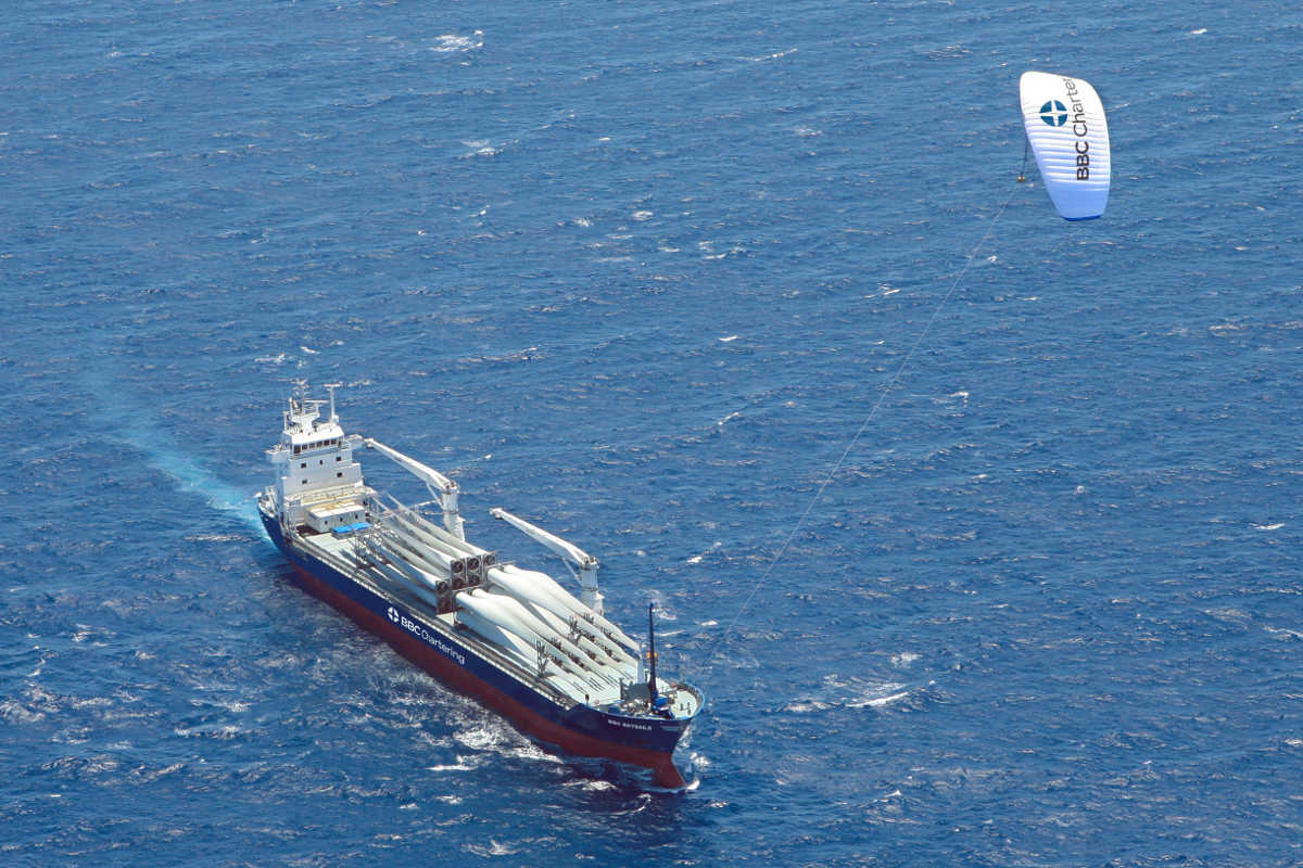
Figure 1: The BBC SkySails with towing kite. The 132 m vessel utilizes kites of sizes up to 320 m².

and Fig. 2.

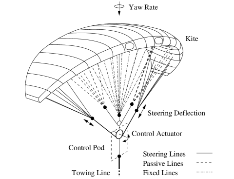
Figure 2: Geometric implementation of the deflection $\delta$ in order to direct the kite. The steering actuator in the control pod drives a tooth belt attached to the kite steering lines as shown in the figure. The main part of the forces is transferred to the control pod by passive and fixed lines. A deflection of the belt warps the kite canopy basically about the roll axis. The resultant dynamics due to aerodynamic forces is mainly a turn rate about the yaw axis which is discussed in detail in Section IV.

The core of the propulsion system is the towing kite steered by the control pod situated under the kite. The towing force is transmitted to the ship by a high-strength synthetic fiber rope. Additionally a launch and recovery system is installed aboard the ship [1]. One key component of the flight control system is the main steering actuator in the control pod applying deflections to some kite lines leading to curve flight.

A control system consisting of distributed computers preprocesses data from various sensors at a rate of 10 Hz and performs the flight control algorithm which calculates the steering command applied to the main actuator. An integrated graphical user interface allows for operation of the system by the crew whereas for research and development purposes prototyping and testing toolchains can be connected via special interfaces.

The paper is organized as follows: First we introduce the basic system and coordinate definitions. We then focus on the main dynamics and develop a model specially suited for controller design. After justification of the main law of the model with experimental data we present our controller design discussing design considerations and controller performance measurements. We complete the article with the explanation of pattern generation.

II Basic System and Coordinates

In this section we give a mathematical description of the considered system. It is worth mentioning that we deal with a constrained system which shows a completely different dynamics compared to free flying parafoils [21]. The basic system is sketched in Fig. 3.

Figure 3: Definition of coordinates for the considered system. The right-handed coordinate system is defined by the basis vectors $\vec{e}_{x},\vec{e}_{y},\vec{e}_{z}$ with $\vec{e}_{x}$ in wind direction and $\vec{e}_{z}$ pointing downwards with respect to gravity. The kite position is parameterized by introducing the spherical coordinates $\varphi$ and $\vartheta$ (for a more precise definition see (2)). The kite axes are labeled as roll $\vec{e}_{\rm roll}$, pitch $\vec{e}_{\rm pitch}$ and yaw $\vec{e}_{\rm yaw}$. This corresponds to the definition usually used in aerospace applications with roll axis parallel to forward and yaw axis parallel to down directions respectively. Note that the yaw vector $\vec{e}_{\rm yaw}$ is defined by the position of the kite assuming it is constrained to the origin by a rigid rod. Thus orientation of the kite is represented by the single angle $\psi$. Detailed vector definitions are given in Appendix A of the paper.

Compared to the real system we make use of some simplifications which are summarized in Table I.

TABLE I: Overview on Model Assumptions used for Setup (Section II) and Dynamics (Section III)

Masses neglected	Usually the aerodynamic forces are larger than system masses and thus acceleration effects play a minor role. The system can be considered to be in equilibrium flight state. This assumption simplifies the equations of motion significantly.
	Apart from exceptional situations the towing rope acts as rigid tether and is considered as massless tether only. Winching during launch and recovery is not considered in this paper.
Aerodynamics	The aerodynamics of the kite is reduced to two assumptions. First we assume the kite is always in its aerodynamic equilibrium which means that the air flow is determined by the glide ratio $E$ (compare Appendix A). Secondly the response to a steering deflection can be described mainly by one parameter $g$ as we show by experimental data in Section IV.
Wind field	We assume a constant and homogeneous wind field with velocity $v_{0}$ to derive the equations. As this assumption often does not hold for real situations we either use the average wind speed at flight altitude, which has to be estimated, for $v_{0}$ or — as done for the controller setup — the air path speed $v_{\rm a}$ (see Appendix B).
	As forward force optimization is not treated in this paper, course and speed of the vessel can be easily eliminated by considering them in the relative wind speed and direction.

The flexible rope is substituted by a rigid rod which also is parallel to the kite yaw axis $\vec{e}_{\rm yaw}$ and all masses are neglected. At first view this seems to be an unrealistic simplification, but the usual mode of operation is the highly dynamical pattern flight leading to line forces large compared to system masses. Therefore inertia effects or free flight situations, where the towing line is no longer stretched out due to gusts or wave induced ship motions, are infrequent. Although consideration of these issues becomes important at a certain point when bringing the system to higher perfection, a detailed description of the solution to these off-nominal situations would go beyond the scope of this paper.

We would like to start with a demonstrative and introductive example to motivate the idea of the chosen coordinate system $\varphi,\vartheta$ and to explain the basic dynamics. Imagine a kite flying in a wind tunnel experiment conducted on a space station which means the absence of gravity. We further assume the free manoeuvrability of the kite unrestricted by obstacles like ground or ceiling. From this mental picture it would be natural to chose a coordinate system with symmetry axis in wind direction. A kite with its roll axis $\vec{e}_{\rm roll}$ antiparallel to the wind direction would stay at a some arbitrary, stationary position like e.g. ’A’, see Fig. 4.

Figure 4: Flying a kite in a fictitious wind tunnel on a space station would be instructive in understanding the basic equations. While the neutral flight is stationary at any arbitrary position like for example A, a constant $\psi\neq 0$ due to steering will lead to a circular orbit B. The diameter is a function of the $\psi$ magnitude. See also Fig. 5 for further illustration.

However, once a deflection is commanded, the kite will go ’down’ and orbit around permanently on a circular path ’B’. The diameter of the steady state circle is a function of our coordinate $\psi$ which in turn is determined by the commanded deflections. The smaller the diameter of the circle the faster flies the kite and thus the more force will be generated. The corresponding dynamical equations will be discussed in detail in Section III.

We would like to emphasize that the above sketched model is our controller design model while we use for various other development and test issues a sophisticated simulator model including multi-body dynamics which also captures the aerodynamical effects more comprehensively (comparable in structure to [22]). Yet, we suggest above model based on this imaginary space station experiment because it is specifically suited for the controller design purpose. It neglects gravity effects and by this a new symmetry axis is gained. The main benefit of this symmetry compared to other coordinate systems [4, 23, 24] is the resulting simplicity of equations of motion which allows us to approach the feedback and guidance design task to a large extent analytically or semi-analytically at least. Further on it provides a straight forward way of describing flight patterns.

Our choice of the design model led to a controller structure to be presented in sections V–VII. This controller structure turned out to work quite effectively in numerous sea trials.

We close this section by definitions for the quantities used in the following. The coordinate system is shown in figure 3. For a constant line length $L$ the state of the kite is defined by the three angles $\varphi,\vartheta$ and $\psi$. With respect to the basis vectors $\vec{e}_{x}$, $\vec{e}_{y}$, $\vec{e}_{z}$ we obtain for the kite position $\vec{x}$:

$$\vec{x}=L\left(\begin{array}[]{c}\cos\vartheta\\ \sin\varphi\sin\vartheta\\ -\cos{\varphi}\sin\vartheta\end{array}\right).$$ (1)

The kite axes are denoted as $\vec{e}_{\rm roll}$ (roll or longitudinal), $\vec{e}_{\rm pitch}$ (pitch) and $\vec{e}_{\rm yaw}$ (yaw). An explicit definition of these vectors is given in Appendix A.

For a description using rotation matrices one would start with a kite at position $L\vec{e}_{x}$ with roll-axis in negative $z$-direction $\vec{e}_{\rm roll}=-\vec{e}_{z}$ and then apply the following rotations: $-\psi$ about $x$, $\vartheta$ about $y$ and finally $\varphi$ about $x$. This transformation reads:

$$R=R_{x}(\varphi)R_{y}(\vartheta)R_{x}(-\psi).$$ (2)

One could interpret the angle $\psi$ as orientation of the kite longitudinal axis with reference to the wind. For a given kite position $\vec{x}$ (parameterized by $\varphi$ and $\vartheta$) the reference orientation $\psi=0$ corresponds to the minimum of the scalar product $\left(\vec{e}_{\rm roll},\vec{e}_{x}\right)$ obtained when turning the kite fixated at this position $\vec{x}$ around its yaw axis $\vec{e}_{\rm yaw}$. A nonzero value $\psi$ represents a kite orientation obtained by a rotation of $\psi$ about the yaw axis $\vec{e}_{\rm yaw}$ starting at this reference orientation.

III System Dynamics used for Design

For verification and other development purposes we use a full dynamics simulation containing a multi-body model, an aerodynamic database and parameters adopted to results of sea trials. In this section we would like to present the main relations and the dynamics of a complementary model specifically tailored for the design of the controller. The detailed derivation steps are summarized in Appendix A.

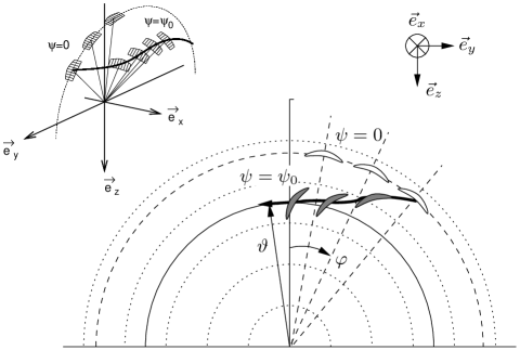
Figure 5: Zenith positions for neutral flight with low force. With $\psi=0$ the parameter $\varphi$ can be freely chosen determining the positions (drawn as white kites). For constant $\psi$ the resulting $\vartheta$ converges as shown by the gray kites flying on the marked trajectory.

The equations of motion for $\vartheta$ and $\varphi$ read:

$$\dot{\vartheta} = \frac{v_{\rm a}}{L}\left(\cos\psi-\frac{\tan\vartheta}{E}\right)$$ (3)

$$\dot{\varphi} = -\frac{v_{\rm a}}{L\sin\vartheta}\sin\psi.$$ (4)

Thus the dynamic is mainly controlled by the angle $\psi$. Further quantities are the air path speed $v_{\rm a}$, the towing line length $L$ and the glide ratio $E$. As already pointed out and to be reasoned in the next section we neglect acceleration and gravity effects in order to obtain these simple equations of motion which allow for the following interpretations.

Detailed computation steps for the subsequent two steady state solutions are given in Appendix A. First, for constant $\psi$, we get a flight trajectory on a circle with constant angle $\vartheta_{0}$ given by

$$\vartheta_{0}(\psi)=\arctan(E\cos\psi).$$ (5)

This equation also applies to the fictitious space station experiment introduced in Section II and Fig. 4. A further result is the dependence of the (steady state) air path velocity $v_{\rm a}$ on the value of $\psi$ and the ambient wind speed $v_{0}$,

$$v_{\rm a}=v_{0}E\cos\vartheta=v_{0}E\cos(\arctan(E\cos\psi))$$ (6)

which is the key issue for pattern generation as we can use $\psi$ as a tuning knob to control $v_{\rm a}$ and the force which is proportional to $v_{\rm a}^{2}$ accordingly. It is worth mentioning that for practicing the sport of kite surfing, the content of (6) is crucial in order to control forces: kite surfers know the angle $\vartheta$ as position in the so called ’wind window’ and the deeper they fly their kite into this ’wind window’ — i.e. they decrease this angle — the more traction force they get and vice versa.

A special case is the so called zenith position for $\psi=0$, a neutral flight situation which generates only low forces and thus is used mainly for launching and recovering the kite. From (5) we get $\vartheta_{0}=\arctan(E)$ and $\varphi$ can be used as free parameter to determine the neutral flight position (compare Fig. 5).

While all equations up to here follow straightforward from kinematic reasoning, albeit the choice of the coordinate system was not ’typical’, the dynamic response of the kite to a steering deflection $\delta$ is claimed to be

$$\dot{\psi}_{\rm m}=g\,v_{\rm a}\,\delta$$ (7)

where $g$ is the proportionality factor and an illustration of the deflection $\delta$ is given in Fig. 2.

We would like to draw special attention to this turn rate law (7) and will show in the following that it can be justified by measured data to a surprising high degree. Therefore it is a key issue for the cascaded controller approach where it constitutes the dynamics of the inner loop.

Finally we would like to point out that due to its motion on a spherical surface an inertial sensor measures a turn rate $\dot{\psi}_{\rm m}$ about the yaw axis $\vec{e}_{\rm yaw}$ different from the derivation $\dot{\psi}=d\psi/dt$. The rotation measured by the pod sensors can be calculated by transforming the dynamics represented by $\dot{R}$ into the pod coordinate system by applying (2). Comparing the rotation operation $\vec{\Omega}\times$ with $R\!\cdot\!\dot{R}^{T}$ yields:

$$\dot{\psi}_{\rm m}=\dot{\psi}-\dot{\varphi}\cos\vartheta.$$ (8)

By consideration of typical flight situations where either $\varphi$ is kept constant during the neutral flight mode or $\dot{\varphi}\propto v_{\rm a}/L$ becomes small due to the long line length $L$ needed for dynamic pattern flight, one can assure oneself that the second term of this equation usually is small compared to the first and thus can be neglected in the first instance and treated as a correction to the controller design later.

We would like to conclude this section by emphasizing that we presented a novel model based on three state variables $\psi$, $\vartheta$, $\varphi$ and three equations of motion (7), (3), (4) whereas previously published models [2], [3], [11], [16] introduce at least four or more state variables. For a summary and further discussion of the equations we refer to Appendix B.

IV Justification of the Turn Rate Law

In this section a justification of (7) is given based on numerous experiments showing the strong proportionality. It is worth noting that (7) is confirmed by measurements to a high degree even in disturbed sea trial conditions. The key issue of these experiments is to perform bang-bang flights which will be presented and discussed in the following.

The excitation of the system for the identification is performed in the following way: We apply a constant steering command $+\delta_{0}$ to the system. The system will respond with a positive yaw rate ($\dot{\psi}_{\rm m}\!>\!0$). When reaching a certain threshold $\psi_{\rm m}\!\geq\!\psi_{0}$ the corresponding opposite steering deflection $-\delta_{0}$ is commanded leading to a decrease of $\psi_{\rm m}$. Falling below the negative threshold $\psi_{\rm m}\!\leq-\!\psi_{0}$, the primary deflection $\delta_{0}$ is commanded again. The schedule of the bang-bang experiments is as follows: the human pilot flies the kite into a high zenith position with $\varphi\!\approx\!0$ and hands over the steering to the computer based control system which performs the described algorithm.

A typical flight trajectory is shown in Fig. 6.

Figure 6: Flight trajectory under computer control for the bang-bang flight experiment. Angles were measured by tow point sensors on the ship determining the direction of the towing rope.

The bang-bang steering leads to a figure-eight-pattern and for typical parameters the air path speed and thus the size of the pattern increase because the kite flies down to smaller elevation angles $\vartheta$. The human pilot only has the task to supervise the flight and overtake manual control before the system runs into the danger of overload or bounces against the water surface.

In Fig. 7 data points for one experiment run are shown. This experiment was performed in 2006 using a 20 m² kite.

Figure 7: Measured data of a bang-bang flight. Yaw rate $\dot{\psi}_{\rm m}$ as function of the air path speed multiplied by deflection $v_{\rm a}\delta$ to justify (7). The parameter $g$ is obtained by the shown linear fit.

Repeating this experiment with different $\delta_{0}$ leads to similar $g$ values and thus proves the validity of (7).

Although the linear dependence can be clearly identified in Fig. 7 it is even more convincing to present the data in the time domain as shown in Fig. 8. Here we compare the time-series of the steering command with the turn rate of the kite. The trapezoidal shape is due to the finite steering velocity of the control pod. The resulting measured yaw rate $\dot{\psi}_{\rm m}$ shows an increase which results from the increasing air path velocity $v_{\rm a}$ over the experiment. The yaw rate divided by $gv_{\rm a}$ is also plotted in order to compare it to the steering command. Although a lot of perturbations affect these experiments we observe an excellent correlation. This analysis justifies the validity of (7) to a high degree and recommends its usage as a key role for the controller design.

Figure 8: Comparison of steering command $\delta$ with yaw rate $\dot{\psi}_{\rm m}$ and the yaw rate divided by the air path velocity $\dot{\psi}_{\rm m}/(g\,v_{\rm a})$. Note the increasing rates are due to increasing air path speed $v_{\rm a}$ while going down into the wind window (compare Fig. 6).

At this point we would like to classify and review these bang-bang experiments in a historical context. Following the textbook approach in classical system identification we did a lot of identification flights in the years 2005 and 2006 using separate batch runs in order to characterize the steering behavior of our kites at the various operating points. The experiments were quite cumbersome: perturbations from wind gusts can be comparatively large compared to periodic excitations caused by the deflection commands and the air path velocities were difficult to tune for the different batch runs and desired operating points. As we had to evaluate data from different days with changing environmental conditions and drifting flight properties of our kites we solely could suspect the validity of law (7). But once we switched to a bang-bang flight strategy the real law shows up clearly. This is obvious as one bang-bang experiment varies the parameter $v_{\rm a}$ over a whole range, in one flight alone, lasting only a few tens of seconds and therefore plays a trick on perturbations.

We would like to conclude this section by giving an extended version of (7) which also takes into account the effect of the gravitational force on the turn rate and reads:

$$\dot{\psi}_{\rm m}=g\,v_{\rm a}\,\delta+M\frac{\cos\theta_{\rm g}\sin\psi_{\rm g}}{v_{\rm a}}.$$ (9)

The quantity $\theta_{\rm g}$ denotes the angle between $\vec{e}_{\rm yaw}$ and the $\vec{e}_{x}$-$\vec{e}_{y}$-plane and $\psi_{\rm g}$ the angle between $\vec{e}_{\rm roll}$ and the $\vec{e}_{x}$-$\vec{e}_{y}$-plane.

Because a steering deflection could be regarded as a kite force component into pitch direction $\vec{e}_{\rm pitch}$ subsequently leading to a yaw rate, the gravity force, projected onto the pitch axis by $\cos\theta_{\rm g}\sin\psi_{\rm g}$, should have the same effect. We have shown in this section that the yaw rate is proportional to $v_{\rm a}\,\delta$. This can be attributed to a side force proportional to $v_{\rm a}^{2}\,\delta$ from aerodynamical and design considerations. Transferring this reasoning to the mass term, which is independent from $v_{\rm a}$, we expect a factor of $M/v_{\rm a}$ between the ’gravitational’ side force and the yaw rate. The constant $M$ includes system masses and kite characteristics. As $M$ is positive for our kites we get an instable behaviour and thus have to stabilize $\psi_{\rm m}$ by active control.

As for the usual operation point of dynamic flight we have $(gv_{\rm a})\gg(M/v_{\rm a})$ and thus the second term of (9), which we call ’mass term’, can be neglected for the design of the linear feedback law only to be introduced as correction term via a feedforward path to the controller structure.

As our operational flights under autopilot conditions (during the dynamic flight modes) utilize similar bang-bang like commands, we can use the discussed identification scheme as a standard tool to establish or check the kite parameter during normal operation. During flights a recursive least-square algorithm [25] runs in order to determine the system parameters $g$ and $M$ on-line. We monitor these values for changes which may indicate upcoming material failures in advance and can adapt controller parameters on-line, if necessary, to increase robustness.

After we have convinced ourselves of the validity of (7), we will now present the controller design which is strongly influenced in its structure by the discussed law.

V Controller Design

Most of time the kite is operated in a highly dynamic regime where the air path speed can easily vary by a factor of up to 3–5 within some seconds and the deflection command can change by more than $60\%$. The classical way to approach such a controller design task would be to use a controller structure which specifically aims at time varying, non-linear systems. Non-linear dynamic inversion or non-linear model predictive control could be such candidates. Gain scheduling based on linearized plant models along the trajectory is a further alternative. Actually we tried the latter approach in the beginning but were not satisfied with the achievable robustness. The core of the problem is governed by the fact that it is difficult to execute a classical modeling approach as usually performed in aerospace application. Such an approach would be based on an aerodynamic database covering the full dynamic regime. Performing wind tunnel tests would be expensive and for our larger kites with 160 m² area downright impossible. We also learned that a controller structure where the kite trajectory is given as a set-point directly into a single controller block, which then directly computes the deflection command, lacks robustness due to the above mentioned modeling issue.

Instead we settled for a separation of the overall controller task into ’guidance’ and ’control’. Section VIII describes how the guidance algorithm computes $\psi_{\rm s}$, which is then the input to the controller. However the major distinguishing feature of our autopilot, compared to other approaches we found in the cited literature, is the cascaded controller structure which is based on the model following principle as shown in Fig. 9.

Figure 9: Cascaded controller approach for $\psi$ control implementing the model following structure. Detailed diagrams for the blocks $[{\rm FF}_{\psi}]$, $[{\rm C}_{\psi}]$, $[{\rm FF}_{\dot{\psi}}]$ and $[{\rm C}_{\dot{\psi}}]$ are shown in figs. 14, 13, 10 and 11. The Controller calculates a steering command $\delta$ from the input value $\psi_{\rm s}$ using a measured yaw angle $\psi_{\rm m}$ and yaw rate $\dot{\psi}_{\rm m}$.

The basic idea is to reflect the separation of dynamics (7) and kinematics, as given by $\dot{\psi}=d\psi/dt$, adequately in the controller structure. We can see two cascaded loops in Fig. 9. The inner loop gets a commanded rate $\dot{\psi}_{\rm s}$ as an input and computes the deflection command $\delta$. The outer loop has ${\psi}_{\rm s}$ as input and commands $\dot{\psi}_{\rm s}$ to the inner loop. Before discussing each controller element in detail we summarize all variables used and relate them to measurements in Table II.

TABLE II: Variables for Conroller Design

Control Actuation
$\delta$	Normalized steering deflection (see Fig. 2)
$\delta_{\rm ff}$	Feedforward computed as shown in Fig. 10.
$\delta_{\rm fbk}$	Feedback computed as shown in Fig. 11.
System Dynamics
$\psi$	Orientation angle of kite longitudinal axis $\vec{e}_{\rm roll}$ with respect to the ambient wind (see Section II).
$\psi_{\rm s}$	Setpoint value from guidance (pattern generation)
$\psi_{\rm c}$	Control reference computed as shown in Fig. 14.
$\psi_{\rm m}$	Value based on inertial measurement unit located in the control pod (pod-IMU) and wind direction estimate.
$\psi_{\rm e}$	Control error ($\psi_{\rm e}\!=\!\psi_{\rm m}\!-\!\psi_{\rm c}$)
$\dot{\psi}$	Turn rate about yaw axis
$\dot{\psi}_{\rm ff}$	Feedforward computed as shown in Fig. 14.
$\dot{\psi}_{\rm fbk}$	Feedback computed as shown in Fig. 13.
$\dot{\psi}_{\rm s}$	Setpoint value $\dot{\psi}_{\rm s}\!=\!\dot{\psi}_{\rm ff}\!+\!\dot{\psi}_{\rm fbk}$.
$\dot{\psi}_{\rm c}$	Control reference computed as shown in Fig. 10.
$\dot{\psi}_{\rm m}$	Measured value based on pod-IMU
$\dot{\psi}_{\rm e}$	Control error ($\dot{\psi}_{\rm e}\!=\!\dot{\psi}_{\rm m}\!-\!\dot{\psi}_{\rm c}$)
$\theta_{\rm g}$	Angle between yaw axis and $\vec{e}_{x}$-$\vec{e}_{y}$-plane, based on pod-IMU measurement.
$\psi_{\rm g}$	Angle between roll axis and $\vec{e}_{x}$-$\vec{e}_{y}$-plane, based on pod-IMU measurement.
$v_{\rm a}$	Airpath speed as measured with respect to $\vec{e}_{\rm roll}$ by an anemometer located aboard the control pod.
$K_{\dot{\psi}}$	Current gain ($K_{\dot{\psi}}\!=\!gv_{\rm a}$) between turn rate and deflection $\dot{\psi}=K_{\dot{\psi}}\delta$ (see Section VI)
$T_{1}$	Influence of gravity on yaw rate, see (11).
$\varphi$	Wind window position, see Fig. 5
$\varphi_{\rm m}$	Measured value based on wind direction estimate and angular sensors at ship towpoint which are wave-motion compensated by the ship-IMU.
$\vartheta$	Wind window position, see Fig. 5.
System Parameters
$g$	Proportional gain of the turn rate law (7), for a 160 m2 system we find $g\approx 0.03$–0.05 rad/m.
$M$	Effect of gravitation on turn rate, see (9)
$E$	Glide ratio $L/D$, typically $E=$4–5 in our case.
$L$	Tether line length assumed to be constant as launch and recovery are not considered here.
$\dot{\delta}_{\rm p}$	Steering speed of the control pod (typically 0.3–0.5 1/s)
$v_{0}$	Ambient wind speed defined for model.

VI Controller Inner Loop

From (7) we recognize that the dynamics from deflection to yaw rate can be viewed as a proportional plant, $\dot{\psi}_{\rm m}=K_{\dot{\psi}}\,\delta$, where $K_{\dot{\psi}}=g\,v_{\rm a}$ denotes the gain. Of course we have to realize that $K_{\dot{\psi}}$ is not constant but a function of the air path velocity. We take care of this by employing a feedforward/feedback structure which implements the model following principle: in the feedforward term $[{\rm FF}_{\dot{\psi}}]$ we compute, in an open loop fashion, the deflection command $\delta_{\rm ff}$ necessary to achieve $\dot{\psi}_{\rm s}$ . The feedback control $[{\rm C}_{\dot{\psi}}]$ only acts when there is a remaining control error due to external disturbances or due to unmodeled plant dynamics. An appropriate delay block is necessary in order to capture all the delays from command to actual execution.

With such a feedforward/feedback structure we can accommodate the dependence of the gain $K_{\dot{\psi}}$ from the air path velocity. Fig. 10 provides details of the feedforward controller block. In line with the idea of the model following principle the feedforward block is not limited to linear equations and can accommodate any system description. The extended version of the turn rate law (9)

$$\dot{\psi}_{\rm m}=K_{\dot{\psi}}\,\delta+M\frac{\cos\theta_{\rm g}\sin\psi_{\rm g}}{v_{\rm a}}$$ (10)

can easily be considered. The principal idea is to invert it in order to compute the necessary deflection $\delta_{\rm ff}$.

In addition the block also contains nonlinear elements, like limiters on angle and rate, in order to capture limited pod steering speed and other constraints. That way the commands from the feedforward will never saturate the deflection capability. Around $60\%$ of this range is reserved for the feedforward leaving the remaining $40\%$ for the feedback. This is usually sufficient for the feedback loop to counteract unmodeled plant uncertainties and disturbances.

The mass term from (10) is introduced via

$$T_{1}=\frac{M}{K_{\dot{\psi}}}\,\frac{\cos\theta_{\rm g}\sin\psi_{\rm g}}{v_{\rm a}}.$$ (11)

Figure 10: Details of block $[{\rm FF}_{\dot{\psi}}]$ of the cascaded controller (see Fig. 9). From input value $\dot{\psi}_{\rm s}$ the feedforward value $\delta_{\rm ff}$ and $\dot{\psi}_{\rm c}$ are calculated by using a steering pod model consisting of a limiter and a ratelimiter. Note the translation of rate to command and back via division and multiplication by $K_{\dot{\psi}}$. Various delays in the whole loop are taken into account by a $z^{-n}$ block before the computation of controller reference input $\dot{\psi}_{\rm c}$.

Figure 11: Feedback block $[{\rm C}_{\dot{\psi}}]$ of the cascaded controller (see Fig. 9). The controller mainly consists of a PI feedback on the yaw rate. Note the division by $K_{\dot{\psi}}$, which is a function of the air path speed, thus introducing a nonlinearity into the feedback by transforming the rate command from the PI controller to the command portion $\delta_{\rm fbk}$ which is routed to the steering pod.

Fig. 11 provides the details of the feedback controller block: As the plant has a proportional character the feedback structure is of proportional/integrator (PI controller) type. The output of the PI controller is divided by $K_{\dot{\psi}}$ thus taking the velocity dependence into account. A lowpass is added for noise rejection of the measurement.

Figure 12: Experimental results for the inner loop. In the upper plot the measured yaw rate $\dot{\psi}_{\rm m}$ is compared to $\dot{\psi}_{\rm s}$ and $\dot{\psi}_{\rm c}$. The lower plot compares feedforward $\delta_{\rm ff}$ and feedback $\delta_{\rm fbk}$ controller output signals for a typical dynamical flight situation.

By providing Fig. 12 we illustrate how effective the inner loop actually works. We show how a couple of repeating flight patterns look at the inner loop level. The feedforward command $\delta_{\rm ff}$ moves between $\pm 60\%$ of the available deflection range as can be seen in the lower graph of the figure. The feedback command $\delta_{\rm fbk}$ hardly needs to correct control errors due to unmodeled plant dynamics. Actually this figure is just an alternative account to Fig. 7 in proving the good fit of the turn rate law.

VII Controller Outer Loop

As seen from the outer loop the inner loop has dealt with the aerodynamically influenced part of the dynamics. It now remains for the outer loop controller to achieve a desired ${\psi}_{\rm s}$. The division into feedforward and feedback parts is kept. Figs. 13 and 14 provide further details.

Figure 13: Feedback block $[{\rm C}_{\psi}]$ of the cascaded controller (compare Fig. 9). As the dynamics to be controlled is mainly an integrator, a proportional feedback has been chosen.

Figure 14: Feedforward block $[{\rm FF}_{\psi}]$ details of cascaded controller (see Fig. 9). The steering pod model is included as combination of limiter and ratelimiter. Note that even for step inputs on $\psi_{\rm s}$ the algorithm computes feedforward $\dot{\psi}_{\rm ff}$ and $\psi_{\rm c}$ in a way which is consistent with the capability of the overall dynamics. This is achieved by using an inner feedback loop embedding the steering pod model. Various delays in the whole loop are taken into account by a $z^{-n}$ block controller reference input $\psi_{\rm c}$.

As the plant characteristic is of integrating nature a feedback law with proportional character $[{\rm C}_{\psi}]$, augmented by a lowpass, is sufficient. As before a limiter is also employed. The feedforward block $[{\rm FF}_{\psi}]$ (see Fig. 14) has more elaborate features. Note that the feedforward term features an internal feedback loop. The basic idea is to shape the commanded $\psi_{\rm s}$, even if it is a jump, in such a way that it corresponds to the actual response capabilities of the control pod and kite. We achieve this by employing an internal loop from $\psi_{\rm s}$ to $\psi_{\rm c}$. Note that the two limiters are crucial in shaping the final $\psi_{\rm c}$ evolution. Furthermore we have a nonlinear function inside the loop: $f(x)={\rm sign}(x)\sqrt{2\dot{\delta}_{\rm p}|x|}$. We will stop short in deriving the details of this special feature and refer to Appendix C. Instead we will illustrate it with Fig. 15. The upper part shows how the input command $\psi_{\rm s}$ is shaped into the command $\psi_{\rm c}$ by the non-linear feature of the internal feedback loop. $\psi_{\rm c}$ corresponds to an actually flyable $\psi_{\rm c}$ pattern. $\dot{\psi}_{\rm ff}$ shows the corresponding necessary rate pattern which is fed into the inner loop.

Figure 15: Flight results for the outer loop. The upper plot compares the response of the measured angle $\psi_{\rm m}$ to a given rectangular $\psi_{\rm s}$. The curve $\psi_{\rm c}$ is computed by the internal loop of the feedforward block $[{\rm FF}_{\psi}]$ using a model of the steering pod (compare Fig. 14).

As a conclusion we will summarize the basic design principles of our controller. The first feature is the separation of the dynamics of deflection to rate (7) from the kinematic of rate to angle. This separation allows us to introduce non-linear elements (mainly limiters) at the appropriate places. This way we achieve a shaping of our commanded signals such that they correspond to the limitations of the complete chain from software command over control pod steering to kite movement.

A second characteristical feature is the feedforward/feedback separation which allows us to decouple non-linear elements, as for example the mass term, from the feedback. The feedback loops can then be designed within the realm of linear control theory. Only proportional or integral dynamics remain which can be handled in a classical way. Due to the feedforward/feedback separation the selection of the closed loop bandwidth of the two loops is more concerned with achieving sufficient stability margin than with achieving performance in terms of fast response because this is already mastered by the feedforward.

The next chapter will illustrate the generation of the $\psi_{\rm s}$ command from the desired kite trajectory. Although it could be perceived as just a further cascaded loop we treat it more like the ’guidance’ feature of classical aerospace applications.

VIII Pattern Generation

In this section we describe the dynamic flight mode which is used to generate traction force by flying dynamical patterns in order to obtain high air path speeds and forces. The algorithm utilizes the presented controller design by providing the input value $\psi_{\rm s}$.

In order to explain the main principles we would like to review the space station experiment of Section II. In this model a constant value of $\psi_{\rm s}=+\psi_{0}$ or $-\psi_{0}$ leads to a circular orbit clockwise or counterclockwise dependent on the sign of $\psi_{\rm s}$ and the obtained force can be easily controlled by the value of $\left|\psi_{\rm s}\right|$. For the purpose of line force generation in our space station experiment this would finish our design effort — but in our application we are not able to fly circular orbits as the kite would crash onto the water surface. Thus the solution is to turn around at certain points of the orbit and fly back and forth.

The resulting trajectory of such a scheme is shown in Fig. 16.

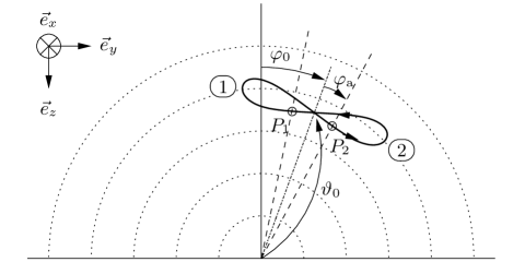
Figure 16: Geometry for pattern generation. The figure-eight pattern is guided by two states (1) and (2). Transitions between those are triggered by the conditions P₁: $\varphi\!<\!\varphi_{0}\!-\!\varphi_{\rm a}$ and P₂: $\varphi\!>\!\varphi_{0}\!+\!\varphi_{\rm a}$. The corresponding sequence is shown in Fig. 17.

The underlying algorithm is similar to those of the bang-bang experiments in Section IV. A constant value $\psi_{\rm s}=+\psi_{0}$ is commanded until point ’P₁’ is reached (at $\varphi\!\leq\!\varphi_{0}\!-\!\varphi_{\rm a}$) triggering the command $\psi_{\rm s}=-\psi_{0}$ until point ’P₂’, then triggering the former value $\psi_{\rm s}=+\psi_{0}$ and so on. The timing of $\psi_{\rm s}$ is depicted in Fig. 17.

Figure 17: Pattern generation sequence toggling between the two states (1) and (2) when conditions P₁: $\varphi\!<\!\varphi_{0}\!-\!\varphi_{\rm a}$ and P₂: $\varphi\!>\!\varphi_{0}\!+\!\varphi_{\rm a}$ are met respectively. The states directly result in a square signal to $\psi_{\rm s}$ which is shaped by the feedforward block $[{\rm FF}_{\psi}]$ into $\psi_{\rm c}$ (compare Section VII). The respective pattern geometry is displayed in Fig. 16.

It is acceptable to apply a square signal to $\psi_{\rm s}$ as the controller design contains an internal model which leads to a calculation of $\psi_{\rm c}$. This calculation utilizes a given curve deflection and the given design speed of the control pod (see Section VII) in order to perform the curve flight. The determination of the optimal curve deflection or optimal turning radius is involved as it depends on several geometric as well as aerodynamic system characteristics [15], [26] and goes beyond the scope of this paper. For our system, the main effect during curve flight is the decrease of air path speed due to the increase of $\vartheta$. Thus curve deflections are typically choosen in the range of 40–70 % of the total deflection range in order to minimize the curve duration and optimize the performance figure.

As illustrated in Fig. 16 there are three parameters defining the trajectory. The parameter $\varphi_{\rm a}$ determines the pattern size; the parameters $\varphi_{0}$ and $\vartheta_{0}$ determine the center point of the pattern. The value $\varphi_{0}$ can be freely chosen within a certain range by the operator or an overlying algorithm in order to optimize the force component pointing in forward direction of the vessel. The value $\vartheta_{0}$ can not be tuned directly but indirectly by the $\psi_{0}$ value which is the tuning knob for the air path speed $v_{\rm a}$ and hence force. Nevertheless (6) does not hold in its simple way and could by improved by using $\left<\psi\right>=\int dt\left|\psi(t)\right|$ instead of $\psi_{0}$ in order to estimate $\vartheta$ or resulting forces.

As it is cumbersome to predict the exact wind situation at flight altitude in any case we make use of another approach for force control: we use an outer loop force controller evaluating the height of the force peaks while flying the figure-eight pattern which provides a feedback value for $\psi_{0}$. Details of this control law as well as of the supervision mechanisms during operative flight and start procedure of the pattern are important and interesting issues each but would exceed the purpose of this paper. In Fig. 18 we present the trajectory of some eights and show the corresponding time series of the angles $\varphi_{\rm m}$, $\psi_{\rm s}$, $\psi_{\rm c}$ as well as of the air path and wind speeds.

Figure 18: Flight test results illustrating pattern generation using a 160 m² kite at an operational towing line length of 300 m. The trajectory for a typical figure-eight pattern is shown in the upper plot (compare Fig. 16). The two plots in the middle show corresponding curves for $\varphi_{\rm m}$, $\psi_{\rm c}$ and $\psi_{\rm m}$ (see Fig. 17). The lower data plot shows the measured wind speeds. Note that the dynamical flight mode leads to an air path speed of factor 3–4 higher than the estimated wind speed at flight altitude which is significantly higher than the wind speed measured aboard the ship.

For sake of completeness we would like to explain the control strategies for the neutral flight mode introduced in Section II. The determining equation is (4) and the issue is to control $\varphi$ to the given set value $\varphi_{0}$. We mainly use a linear controller based on a classical PID controller in order to compute $\psi_{\rm s}$ from $\varphi_{\rm m}\!-\!\varphi_{0}$.

IX Discussion and Further Challenges

Dealing with a complex system in a demanding environment we could present several further topics on our control system which are closely related to the discussed contents. These topics have been omitted in the previous sections because we wanted a clear outline of the major features of the algorithm. They are now briefly summarized to give a more comprehensive understanding.

First of all we have completely excluded the ship from our treatment by arguing that consideration of the apparent wind, which is the wind speed with respect to the ship’s motional frame of reference, is an appropriate approximation for the basic design of the control system. Furthermore the choice of pattern parameters [24], [26] the optimization of the towing force with respect to the ship forward direction [27], [28] as well as consideration of influences on dynamics due to waves are improvements to an operational kite autopilot but have not been presented here.

It is worth mentioning that both, the thorough choice of the sensor set up and preprocessing algorithms, contribute a significant and crucial part to the presented controller performance and robustness. An important task is the estimation of the angle $\psi$ which involves not only sophisticated inertial navigation algorithms but also takes into account estimates for wind speed and wind direction at flight altitude as these may vary on the timescale of minutes. A further discussion of these mainly technical and cumbersome topics will be subject to future publications.

In our discussions we have made use of constant and long line lengths which is the common operating point of our system. Winching of the towing line is done while launching and recovering our system and goes along with extra dynamic effects which are considered as additional correction terms to the presented equations. Especially for control during launch and recovery at shorter line lengths we use the idea of receding horizon feedback from the model predictive control (MPC) approaches [29] in order to provide $\psi_{\rm s}$. However our optimization computation is done analytically (thanks to the special and simple structure of the design model, see III) as opposed to having a numerical solver.

Wind gusts may also go along with downwinds leading to a free flight situation of the usually constrained system. This situation involves a completely different dynamics. While (7) still holds in large part the kinematic changes significantly. It is a crucial advantage of the particular choice of coordinate system (see section II) that controller input values behave in a favorable way during these exceptional occurrences. We would like to note that also disturbances due to excitations of internal modes of the real system are effectively suppressed although these modes are not considered explicitly in the ’design model’.

A more elaborate challenge is the avoidance of and response to stall situations. Systematic experimental tests on this are hardly feasible. Nevertheless it is an important issue and subject to current research and development activities.

X Summary

In this paper we have presented a simple dynamical model for the dynamics of constrained kites. A key point has been that for controller design the complete aerodynamics can be reduced to a law involving only one or two quantities (see (7) and (9), respectively). We have discussed flight data to justify that this reduction describes reality to a surprisingly high degree. Utilizing this we have developed a cascaded controller, based on the model following principle approach, and proved the effectiveness with flight test data. Finally the main principles of flight pattern generation have been given.

We would like to finish this paper by emphasizing that the presented results hold for the SkySails towing kite system but the underlying equations are commonly valid for the dynamics of constrained kites. Thus a lot more applications of the presented controller are feasible especially in the fascinating upcoming field using kites in order to generate electricity and to further open up the green resource of wind power in higher altitudes and off-shore.

Appendix A Derivation of System Dynamics

The system vectors read (see Fig. 3):

$$\vec{e}_{\rm roll} = \left(\begin{array}[]{c}-\sin\vartheta\cos\psi\\ -\cos\varphi\sin\psi+\sin\varphi\cos\vartheta\cos\psi\\ -\sin\varphi\sin\psi-\cos\varphi\cos\vartheta\cos\psi\end{array}\right)$$ (15)

$$\vec{e}_{\rm pitch} = \left(\begin{array}[]{c}\sin\vartheta\sin\psi\\ -\cos\varphi\cos\psi-\sin\varphi\cos\vartheta\sin\psi\\ -\sin\varphi\cos\psi+\cos\varphi\cos\vartheta\sin\psi\end{array}\right)$$ (19)

$$\vec{e}_{\rm yaw} = \left(\begin{array}[]{c}-\cos\vartheta\\ -\sin\varphi\sin\vartheta\\ \cos{\varphi}\sin\vartheta\end{array}\right).$$ (23)

As discussed in Section II we neglect gravity. Thus the problem becomes independent of $\varphi$ and can be treated for $\varphi=0$ without loss of generality which implies the following basis vectors:

$$\vec{e}_{\rm roll} = \left(\begin{array}[]{c}-\sin\vartheta\cos\psi\\ -\sin\psi\\ -\cos\vartheta\cos\psi\end{array}\right)$$ (27)

$$\vec{e}_{\rm pitch} = \left(\begin{array}[]{c}\sin\vartheta\sin\psi\\ -\cos\psi\\ \cos\vartheta\sin\psi\end{array}\right)$$ (31)

$$\vec{e}_{\rm yaw} = \left(\begin{array}[]{c}-\cos\vartheta\\ 0\\ \sin\vartheta\end{array}\right).$$ (35)

The air flow $\vec{v}_{\rm a}$ of the flying system is

$$\vec{v}_{a}=\left(\begin{array}[]{c}v_{0}\\ 0\\ 0\end{array}\right)-v_{\rm roll}\vec{e}_{\rm roll}-v_{\rm pitch}\vec{e}_{\rm pitch}.$$ (36)

The first term describes the external wind, the subsequent two terms the flow due to the kinematic speeds $v_{\rm roll}$ and $v_{\rm pitch}$ with respect to the basis vectors $\vec{e}_{\rm roll}$ and $\vec{e}_{\rm pitch}$.

Considering the basic aerodynamics of an airfoil [21] as a very simple model we claim validity of the following two conditions:

1. The airflow vector lies in the $\vec{e}_{\rm roll}$-$\vec{e}_{\rm yaw}$-plane which means

   $$\left(\vec{e}_{\rm pitch},\vec{v}_{\rm a}\right)=0.$$ (37)

2. The airflow direction with respect to $\vec{e}_{\rm roll}$ and $\vec{e}_{\rm yaw}$ is given by the glide ratio $E$ which is the ratio between lift and drag coefficients $E=L/D$,

   $$\frac{\left(\vec{e}_{\rm roll},\vec{v}_{\rm a}\right)}{\left(\vec{e}_{\rm yaw},\vec{v}_{\rm a}\right)}=E.$$ (38)

Insertion of the definitions (27)–(35) into (37) and (38) yields the velocity components

$$\frac{v_{\rm pitch}}{v_{0}} = \sin\vartheta\sin\psi$$ (39)

$$\frac{v_{\rm roll}}{v_{0}} = E\cos\vartheta-\sin\vartheta\cos\psi.$$ (40)

The airflow in roll direction $v_{\rm a}$, measured by the anemometer in the control pod, can be calculated using (27) and (36) by:

$$v_{\rm a}=-\left(\vec{v}_{\rm a},\vec{e}_{\rm roll}\right)=v_{0}E\cos\vartheta.$$ (41)

Geometric and kinematic considerations lead to the relation

$$\dot{\vartheta}=\frac{1}{L}\left(v_{\rm roll}\cos\psi-v_{\rm pitch}\sin\psi\right).$$ (42)

Using (39), (40) and (41) we get for the dynamics of $\vartheta$ the following differential equation:

$$\dot{\vartheta}=\frac{v_{\rm a}}{L}\left(\cos\psi-\frac{\tan\vartheta}{E}\right).$$ (43)

Similarly we obtain for $\varphi$ the equation

$$\dot{\varphi}=\frac{1}{L\sin\vartheta}\left(-v_{\rm roll}\sin\psi-v_{\rm pitch}\cos\psi\right),$$ (44)

and using (39), (40) and (41) the equation of motion

$$\dot{\varphi}=-\frac{v_{\rm a}}{L\sin\vartheta}\sin\psi.$$ (45)

For constant values of $\psi$, one obtains the steady-state solution of (43) as

$$\vartheta_{0}(\psi)=\arctan(E\cos\psi).$$ (46)

Appendix B Equations of Motion

In this appendix we summarize the equations of motion (7), (43) and (45) for our model

$$\dot{\psi} = g\,v_{\rm a}\,\delta$$ (47)

$$\dot{\vartheta} = \frac{v_{\rm a}}{L}\left(\cos\psi-\frac{\tan\vartheta}{E}\right)$$ (48)

$$\dot{\varphi} = -\frac{v_{\rm a}}{L\sin\vartheta}\sin\psi.$$ (49)

Following our model we find that $v_{\rm a}$ is a function of the ambient wind speed $v_{0}$ and $\vartheta$ (41) and has to be considered as part of the equations of motions:

$$v_{\rm a}=v_{0}E\cos\vartheta.$$ (50)

Before inserting this relation into (47)–(49), we would like to emphasize that $v_{\rm a}$ can be measured directly as a single sensor input instead of using (50). Using $v_{0}$ and $\vartheta$ to determine $v_{\rm a}$ would introduce avoidable inaccuracies into our control loop as in addition to errors in the aerodynamical model and $E$ the wind speed at flight altitude, which should by used for $v_{0}$, is typically (but not necessarily) higher than the wind speed measured aboard the vessel (compare Fig. 18). Computing an estimate for $v_{0}$ at flight altitude involves $v_{\rm a}$ and thus would not provide any benefit compared to using $v_{\rm a}$ directly. In other words (47) represents the physics of the kite reacting to a deflection $\delta$ with a turn rate $\dot{\psi}$ scaled by the airflow speed $v_{\rm a}$ independent of e.g. the position represented by $\vartheta$.

In contrast to an operational control setup a numerical simulation has to compute $v_{\rm a}$ based on $v_{0}$. The set of equations can be combined by inserting (50) into (47)–(49) and we obtain:

$$\dot{\psi} = (g\,v_{0}E\cos\vartheta)\,\delta$$ (51)

$$\dot{\vartheta} = \frac{v_{0}}{L}\left(E\cos\vartheta\cos\psi-\sin\vartheta\right)$$ (52)

$$\dot{\varphi} = -\frac{v_{0}\,E}{L\tan\vartheta}\sin\psi.$$ (53)

Appendix C Function $f(x)$ for $\psi$-Feedforward Block

In this appendix the origin of the nonlinear function $f(x)$ used by the feedforward block in Section VII is briefly outlined. We thereby emphasize that the following is not crucial for an understanding of the main concepts but gives further insight into a model-based detail of the feedforward generation. Assume the process of starting with an initial deflection of $\delta\!=\!\delta_{\rm i}$ and steering to $\delta\!=\!0$ at a constant velocity $\dot{\delta}_{\rm p}$ . The corresponding change in $\psi$ which we denote by $\Delta\psi$ can be computed using (7) as $\Delta\psi\!=\!\int dt\dot{\psi}\!=\!K_{\dot{\psi}}\int dt\,\dot{\delta}_{\rm p}t$ for $t=0..(\delta_{\rm i}/\dot{\delta}_{\rm p})$. Resolving with respect to $\delta_{\rm i}$ yields:

$$\delta_{\rm i}={\rm sign}(\Delta\psi)\sqrt{\frac{2\dot{\delta}_{\rm p}|\Delta\psi|}{K_{\dot{\psi}}}}.$$ (54)

This solution already includes the bookkeeping of signs assuming that $\dot{\delta}_{\rm p}$ is a positive parameter. The interpretation of the result is as follows: for a given deviation $\Delta\psi$ of the internal state to the set point $\psi_{\rm s}$ (compare Fig. 14) a $\delta_{\rm i}$ can be calculated using (54). This $\delta_{\rm i}$ describes the maximum deflection allowed for the internal model so that no overshoots occurs when the internal feedback loop reduces the error $\Delta\psi$ under the assumption of constant $\psi_{\rm s}$ and $K_{\dot{\psi}}$. Thus $\delta_{\rm i}$ is a suitable input for the model shaping elements limiter and ratelimiter in Fig. 14. Finally $f(x)={\rm sign}(x)\sqrt{2\dot{\delta}_{\rm p}|x|}$ can be deduced from comparing (54) to Fig. 14.

Michael Erhard received the Diploma degree from the University of Freiburg, Freiburg, Germany, and the Ph.D. degree, which involved research on multi-component Bose–Einstein condensates, from the University of Hamburg, Hamburg, Germany, in 2000 and 2004, respectively, both in physics. His research interests included experiments in quantum optics, laser physics, and theoretical quantum optics. He joined SkySails GmbH, Hamburg, Germany, in 2004, as a Development Engineer, where he was deeply involved in several hardware and software designs on the sensor data acquisition system and the kite steering units. He is currently in charge of the flight control system (autopilot). His main responsibility is the development of sensor data processing and control algorithms for the flying system and evaluation of those algorithms in flight tests.

Hans Strauch received the Diploma degree in physics (1981) from the University of Kiel, Kiel, Germany. He joined Anschütz GmbH, Kiel, where he was involved in the development of autopilots and ground track controllers for ships. In 1988, he joined Astrium Space Transportation, Bremen, Germany, where he was involved in development of the guidance and control algorithms for various vehicles ranging from upper stages of launchers to re-entry bodies. He is currently holds a Senior Expert GNC. From 1998 to 2002, he was with NASA, Johnson Space Center, Houston, TX, where he was involved in the development of guidance and control software for the parafoil phase of the X38 Crew Rescue Vehicle. In 2004, he was responsible for the attitude control of the winged body autonomous landing demonstrator PHOENIX. He has been a Consultant with SkySails GmbH, Hamburg, Germany since 2004. His contributions to the findings reported in this paper are independent from his affiliation to Astrium.

References

- [1] SkySails GmbH. [Online]. Available: http://www.skysails.de
- [2] M. Canale, L. Fagiano, and M. Milanese, “Power kites for wind energy generation,” IEEE Control Syst. Mag., pp. 25–38, Dec. 2007.
- [3] L. Fagiano, M. Milanese, and D. Piga, “High altitude wind power generation,” IEEE Trans. Energy Convers., vol. 25, no. 1, pp. 168–180, 2010.
- [4] P. Williams, B. Lansdorp, R. Ruiterkamp, and W. Ockels, “Modeling, simulation, and testing of surf kites for power generation,” Proc. Modelling and Simulation Technologies Conf. AIAA 2008-6693, Aug. 2008.
- [5] KITEnrg Altitude Wind Generation. [Online]. Available: http://www.kitenergy.net
- [6] EnerKite GmbH. [Online]. Available: http://www.enerkite.de
- [7] SwissKitePower collaborative Research and Development Project. [Online]. Available: http://www.swisskitepower.ch
- [8] Makani Power Inc. [Online]. Available: http://www.makanipower.com
- [9] Ampyx Power. [Online]. Available: http://www.ampyxpower.com
- [10] “Book of abstracts,” ISBN 978-94-6018-370-6, Airborne Windenergy Conference 2011. [Online]. Available: http://www.awec2011.com
- [11] A. Ilzhöfer, B. Houska, and M. Diehl, “Nonlinear MPC of kites under varying wind conditions for a new class of large scale wind power generators,” Int. J. Robust Nonlinear Control, vol. 17, no. 17, pp. 1590–1599, Nov. 2007.
- [12] P. Williams, B. Lansdorp, and W. Ockels, “Optimal crosswind towing and power generation with tethered kites,” AIAA Journal of Guidance, Control and Dynamics, vol. 31, no. 1, pp. 81–93, Jan. 2008.
- [13] ——, “Nonlinear control and estimation of a tethered kite in changing wind conditions,” AIAA Journal of Guidance, Control and Dynamics, vol. 31, no. 3, pp. 793–799, 2008.
- [14] A. Furey and I. Harvey, “Evolution of neural networks for active control of tethered airfoils,” Proc. The 9th European Conference on Artificial Life, pp. 746–756, 2007.
- [15] L. Fagiano, “Control of tethered airfoils for high-altitude wind energy generation,” Ph.D. dissertation, Politecnico di Torino, Italy, 2009.
- [16] B. Houska and M. Diehl, “Robustness and stability optimization of power generating kite systems in a periodic pumping mode,” Proc. of the IEEE Multi-Conference on Systems and Control, Sep. 2010.
- [17] J. H. Baayen and W. J. Ockels, “Tracking control with adaption of kites,” IET Control Theory and Applications, vol. 6, no. 2, pp. 182–191, 2012.
- [18] G. Dadd, “Development, validation, and demonstration of a test rig for kite performance,” Master’s thesis, University of Southampton, GB, 2001.
- [19] B. Lansdorp, R. Ruiterkamp, and W. Ockels, “Towards flight testing of remotely controlled surfkites for wind energy generation,” Proc. Modelling and Simulation Technologies Conf. AIAA-2007-6643, Aug. 2007.
- [20] M. Canale, L. Fagiano, and M. Milanese, “High altitude wind energy generation using controlled power kites,” IEEE Trans. Control Syst. Technol., vol. 18, no. 2, pp. 279–293, 2010.
- [21] J. S. Lingard, “The aerodynamics of gliding parachutes,” Proc. 9th Aerodynamics Decelerator and Ballon Tech. Conf., AIAA-86-2427-CP, Oct. 1986.
- [22] P. Williams, B. Lansdorp, and W. Ockels, “Flexible tethered kite with moveable attachment points, part I: Dynamics and control,” Proc. Atmospheric Flight Mechanics Conf. AIAA-2007-6628, Aug. 2007.
- [23] M. Diehl, “Real-time optimization for large scale nonlinear processes,” Ph.D. dissertation, University of Heidelberg, Germany, 2001.
- [24] G. M. Dadd, D. A. Hudson, and R. A. Shenoi, “Determination of kite forces using three-dimensional flight trajectories for ship propulsion,” Renewable Energy, vol. 36, pp. 2667–2678, 2011.
- [25] L. Ljung, System Identification, 2nd ed. Prentice Hall PTR, 2007.
- [26] L. Fagiano, M. Milanese, and D. Piga, “Optimization of airborne wind energy generators,” Int. J. Robust. Nonlinear Control, 2011. [Online]. Available: http://dx.doi.org/10.1002/rnc.1808
- [27] B. Houska and M. Diehl, “Optimal control of towing kites,” Proc. IEEE Conference on Decision and Control, pp. 2693–2697, 2006.
- [28] L. Fagiano, M. Milanese, V. Razza, and M. Bonansone, “High-altitude wind energy for sustainable marine transportation,” IEEE Trans. Intell. Transp. Syst., vol. 13, pp. 781–791, Jun. 2012.
- [29] J. M. Maciejowski, Predictive Control - with Constraints, 1st ed. Prentice Hall PTR, 2002.