Jet-driving protostars identified from infrared observations of the Carina Nebula complex

Abstract

Aims. Jets are excellent signposts for very young embedded protostars, so we want to identify jet-driving protostars as a tracer of the currently forming generation of stars in the Carina Nebula, which is one of the most massive galactic star-forming regions and which is characterised by particularly high levels of massive-star feedback on the surrounding clouds.

Methods. We used archive data to construct large $(\ga 2\degr\times 2\degr$) Spitzer IRAC mosaics of the Carina Nebula and performed a spatially complete search for objects with excesses in the 4.5  $\upmu\mathrm{m}$ band, typical of shock-excited molecular hydrogen emission. We also identified the mid-infrared point sources that are the likely drivers of previously discovered Herbig-Haro jets and molecular hydrogen emission line objects. We combined the Spitzer photometry with our recent Herschel far-infrared data to construct the spectral energy distributions, and used the Robitaille radiative-transfer modelling tool to infer the properties of the objects.

Results. The radiative-transfer modelling suggests that the jet sources are protostars with masses between $\sim 1\,M_{\odot}$ and $\sim 10\,M_{\odot}$ that are surrounded by circumstellar disks and embedded in circumstellar envelopes.

Conclusions. The estimated protostar masses $\leq 10\,M_{\odot}$ suggest that the current star-formation activity in the Carina Nebula is restricted to low- and intermediate-mass stars. More optical than infrared jets can be observed, indicating that star formation predominantly takes place close to the surfaces of clouds.

1 Introduction

Most stars in the Galaxy are born in massive star-forming regions. The high-mass stars profoundly influence their environments by their strong ionising radiation and powerful stellar winds that can disperse the natal molecular clouds. However, ionisation fronts and expanding wind-driven superbubbles can also compress surrounding clouds, thereby possibly triggering the formation of new generations of stars. Although this feedback is fundamental for understanding the star-formation processes, the details of the astrophysical processes at work are still not understood well, mainly because regions with high levels of massive-star feedback are usually too far away for detailed studies.

The Great Nebula in Carina (NGC 3372; see Smith & Brooks 2008, for an overview and full references) provides a unique target for studies of massive-star feedback. The Carina Nebula complex (hereafter CNC) is located at a moderate and very well-determined distance of 2.3 kpc. With 70 known O-type and Wolf-Rayet stars (Smith 2006) – among them several of the most massive ($M\ga 100\,M_{\odot}$) and luminous stars known in our Galaxy – it represents the nearest southern region with a large massive stellar population.

The presence of these very massive stars implies a very high level of stellar feedback in the CNC. At the same time, the comparatively small distance to the CNC guarantees that we still can study details of the cluster and cloud structure at sufficient spatial resolution so as to detect and characterise the low-mass stellar populations.

During the past few years, several large surveys of the CNC have been performed. The Chandra X-ray observatory obtained a deep wide-field ($\sim 1.4\,\deg^{2}$) X-ray survey of the Carina complex (see Townsley et al. 2011b) that led to the detection of 14 368 X-ray point sources (Broos et al. 2011b), as well as copious amounts of diffuse X-ray emission (Townsley et al. 2011a). The analysis of the X-ray and infrared properties of the point sources suggested that 10 714 objects are young stars in the CNC (Broos et al. 2011a), providing, for the first time, a large (but luminosity-limited) sample of the young stellar population in the area.

A very deep near-infrared survey of the central 1280 square-arcminute area performed with HAWK-I at the ESO 8 m Very Large Telescope (Preibisch et al. 2011b) has revealed more than 600 000 infrared sources. The combination of this infrared catalogue with the list of X-ray sources provides new insight into the properties of the stellar populations in the CNC (Preibisch et al. 2011a).

Spitzer infrared surveys located numerous embedded young stellar objects (YSOs) throughout the CNC (Smith et al. 2010b; Povich et al. 2011). A large ($\sim 1.5\,\deg^{2}$) sub-mm survey of the CNC (Preibisch et al. 2011c) provided essential information about the structure and properties of the cold clouds.

In combination with previous results, these new surveys have yielded very interesting information about the star-formation process in the Carina Nebula. The feedback of the numerous massive stars has already largely dispersed the original molecular clouds in the central region of the Carina Nebula. A few parsecs from the centre, however, large amounts of rather dense clouds are still present. Infrared images show how these clouds are currently eroded and shaped by the radiation and winds from the massive stars, giving rise to numerous giant dust pillars, especially in the so-called “South Pillars” region (Smith et al. 2010b), but also in the clouds northwest of $\upeta$ Car. Several very young stellar objects (e. g. Mottram et al. 2007) and a spectacular young embedded cluster (the “Treasure Chest Cluster”; see Smith et al. 2005) have been found in the molecular clouds, providing clear evidence that vigorous star formation activity is going on in these irradiated clouds. It is thought that the formation of these objects was triggered by the advancing ionisation fronts that originate from the (several Myr old) high-mass stars in the CNC (Smith et al. 2010b; Povich et al. 2011). While this scenario appears very reasonable and is supported by recent numerical simulations of the evolution of irradiated clouds (e. g. Gritschneder et al. 2010), the existing data cannot provides clear proof of the triggered–star-formation scenario. The alternative explanation that stars form spontaneously everywhere in the clouds (i. e. independent of external influences) and are only revealed by the advancing ionisation fronts (that simply remove the clouds surrounding the newly formed stars) cannot be ruled out. If it was possible to show that star formation is spatially restricted to the irradiated surface of the clouds (where the radiation pressure is highest), this would provide a very substantial argument in favour of the triggered star formation scenario.

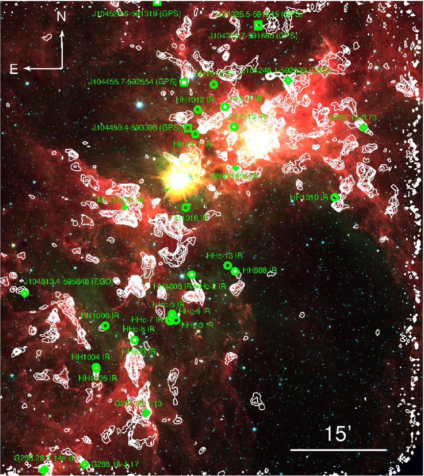
Figure 1: Spitzer RGB image with overlaid LABOCA 870 $\upmu\mathrm{m}$ contours, shown for the same field as in Smith et al. (2010a) for identifying Herbig-Haro jets. The first three contour levels are 0.06, 0.12, and 0.18 Jy/beam, while the further levels increase by a factor of the square root of two. The jet sources in the region are marked in green. Circles indicate sources of HH jets and candidates, diamonds those of EGOs, and squares compact green objects. The sources of MHOs are marked by crosses.

However, the results so far do not allow drawing strong conclusions about the spatial distribution of the currently forming stars. While the infrared data are deep enough to detect the young stellar objects in the CNC easily, major problems arise from the very high level of field-star contamination that is a consequence of the CNC’s location almost exactly on the galactic plane. Only a few percent of all infrared sources seen in the Spitzer and HAWK-I images are actually young stellar objects related to the CNC, while the vast majority are background contaminants (see discussion in Smith et al. 2010b; Povich et al. 2011; Preibisch et al. 2011b).

The main problem in any study of the star-formation process in the CNC thus is not to detect the YSOs, but to discern YSOs in the CNC from background sources. In this context, protostellar jets provide a very good signpost for YSOs, as they point towards objects in the latest generation of the currently forming stars (see Bally et al. 2007). The spatial distribution of jet-driving protostars can thus provide very important information about the regions where star formation presently occurs. These protostars are so young that they are still located very close to their birth site, which means that the jet-driving YSOs trace the spatial location of the currently forming YSO population.

In the strong shocks within the jet flows, or at locations where the jet impacts surrounding clouds, the gas is strongly heated and collisionally excited. This can result in strong, shock-excited line emission, depending on the state of the flowing material and the surrounding clouds. Jets propagating in the diffuse, atomic gas outside the dense molecular clouds often produce prominent atomic emission lines, such as H$\alpha$ or [SII], that can be easily observed in optical images and are known as Herbig-Haro (HH) objects (see Reipurth & Bally 2001). If, on the other hand, the jet propagates within a dense molecular cloud, emission from collisionally excited molecular hydrogen is often seen. The radiative decay of the excited molecules via ro-vibrational transitions produces strong emission lines in the near- and mid-infrared wavelength range.

The 2.12 $\upmu\mathrm{m}$  $\nu=1\!-\!0$  S(1) ro-vibrational emission line of molecular hydrogen is one widely used tracer of these shocks (e. g., McCaughrean et al. 1994; Smith et al. 2007; Davis et al. 2008). The Spitzer IRAC band 2, centred at 4.5  $\upmu\mathrm{m}$, contains several strong H₂ lines, including the transitions $\nu=2\!-\!1$ O(7), $\nu=0\!-\!0$ S(11), $\nu=0\!-\!0$ S(10), $\nu=2\!-\!1$ O(8), $\nu=1\!-\!0$ O(9), $\nu=0\!-\!0$ S(9), and $\nu=0\!-\!0$ S(8). This is why jets often appear as prominent green nebulae in Spitzer RGB images when the 4.5 $\upmu\mathrm{m}$ image is used for the green colour channel (see e. g. Gutermuth et al. 2008). These objects are often denoted as “extended green objects” (EGOs) or “green fuzzies”.

Three recent searches for jets have been performed in the CNC. Smith et al. (2010a) used the ACS camera on the Hubble Space Telescope (HST) to perform a deep H$\upalpha$ narrow-band imaging survey of a $13.6\arcmin\times 27\arcmin$ region in the centre of the Carina Nebula, as well as several non-contiguous pointings at various positions in the Nebula. They detected 40 HH jets and HH jet candidates within the $\sim 0.8\degr\times 1.1\degr$ area that was partly covered by their observations (see their Fig. 1). Smith et al. (2010b) analysed the Spitzer data of the South Pillars within the CNC and identified four EGOs.

In the context of the HAWK-I near-infrared survey of the central $\sim 1280$ square-arcminute region of the CNC described in Preibisch et al. (2011b), we used images obtained through a narrow-band filter centred on the 2.12  $\upmu\mathrm{m}$  $\nu=1\!-\!0$  S(1) ro-vibrational emission line of molecular hydrogen to search for molecular hydrogen emission-line objects (MHOs). This resulted in the detection of six MHOs, which are listed as MHO 1605 to 1610 in the “Catalogue of Molecular Hydrogen Emission-Line Objects in Outflows from Young Stars”.

In this paper, we are going to extend the search for jets and their driving protostars to the full area of the CNC ($\sim 1\,\deg^{2}$ around $\upeta$ Car as shown in Fig. 1). In the first step, we use the large Spitzer IRAC mosaics we have created from available archive data, which provide a spatially complete coverage of the entire extent of the CNC, to search for more objects with 4.5 $\upmu\mathrm{m}$ excess emission, beyond the EGOs already detected by Smith et al. (2010b). In the second step, we identify the driving sources of the newly detected jets and the known HH jets and MHOs in the Spitzer images (Sect. 3). Using the tools developed by Robitaille et al. (2006, 2007), we fit the spectral energy distributions (SEDs) of the jet sources by combining Spitzer photometry with far-infrared fluxes derived from our very recent Herschel mapping and our previous LABOCA sub-mm study of the CNC (Preibisch et al. 2011c). We derive estimates of the stellar and circumstellar parameters of the jet sources by radiative-transfer modelling of the SEDs and investigate the spatial distribution of the jet-driving protostars (Sect. 4) to infer information about the star formation mechanisms currently at work in the Carina Nebula.

2 Observational data

We used the following infrared data sets firstly to search for jet sources and secondly to determine source fluxes to construct their SEDs for the radiative transfer modelling as described in Sect. 4.1.

2.1 Spitzer images and photometry

The data used here were taken during the Spitzer cold mission phase, in July 2008, with the InfraRed Array Camera (IRAC; Fazio et al. 2004) (”Galactic Structure and Star Formation in Vela-Carina” programme; PI: Steven R. Majewski, Prog-ID: 40791). They were retrieved through the Spitzer Heritage Archive. Using the MOsaicker and Point source EXtractor package (MOPEX; Makovoz & Marleau 2005) software provided by the Spitzer Science Center (SSC), we assembled the basic calibrated data into mosaics covering the area around $\upeta$ Car, incorporating the whole extent of the central Carina nebula.

For these IRAC mosaics we performed photometry using the Astronomical Point source EXtractor (APEX) module of MOPEX. During the process, photometry was carried out individually for each image in the stack and combined internally to provide photometry data for the entire mosaic. Point response functions (PRFs) for this purpose are available from the SSC and the appropriate set of PRFs for the time of the observations was employed. Outliers were removed using the Box Outlier Detection method within MOPEX and backgrounds between the tiles were matched using the Overlap module before the mosaics were constructed.

Three Spitzer astronomical observation requests (AORs) each were merged before performing aperture photometry on the constructed mosaics for all four IRAC bands (3.6 $\upmu\mathrm{m}$, 4.5 $\upmu\mathrm{m}$, 5.8 $\upmu\mathrm{m}$, and 8.0 $\upmu\mathrm{m}$) separately. Finally, with the Bandmerge program provided by the Spitzer Science Center  an overall catalogue was created that contained all sources detected with IRAC in the area, their positions and fluxes in all four bands, retaining the information of the detection bands per source. Our catalogue agrees well with the catalogue constructed by Smith et al. (2010b) within the area where both overlap. Source positions, as well as measured fluxes, are in good concordance between the two catalogues. The root mean square (RMS) deviation in magnitudes for sources is 0.092 mag in the 4.5 $\upmu\mathrm{m}$ band, 0.13 mag in the 3.6 $\upmu\mathrm{m}$ band and 0.17 mag in the two longest-wavelength bands.

The one-sigma sensitivity limits for Spitzer for a high background as in the present case given in the IRAC Instrument Handbook are 34, 41, 180, and $156\,\upmu$J for 3.6 $\upmu\mathrm{m}$, 4.5 $\upmu\mathrm{m}$, 5.8 $\upmu\mathrm{m}$, and 8.0 $\upmu\mathrm{m}$, respectively. The exact values depend on the background, which within our field varies strongly.

For this study, we focused on the area of around one square degree as shown in Fig. 1, the same area as analysed in Smith et al. (2010a). One EGO slightly north of this area is included in the study.

2.2 Herschel far-infrared fluxes

For further characterisation of the jet sources, we included fluxes extracted from the data of our recent Herschel far-infrared survey of the CNC. These observations were performed in December 2010 (Open time project, PI: Thomas Preibisch, Prog-ID: OT1-tpreibis-1), using the parallel fast scan mode at $60\arcsec\mathrm{s}^{-1}$. With simultaneous five-band imaging with PACS (Poglitsch et al. 2010) at 70 $\upmu\mathrm{m}$ and 160 $\upmu\mathrm{m}$ and SPIRE (Griffin et al. 2010) at 250 $\upmu\mathrm{m}$, 350 $\upmu\mathrm{m}$ and 500 $\upmu\mathrm{m}$ two orthogonal scan maps were obtained to cover an area of $2.3\times 2.3\deg^{2}$. A full description of these observations and the subsequent data processing will be given elsewhere.

Herschel fluxes were only extracted for cases where a compact, point-like Herschel object could be found at the position of the Spitzer source. No photometry was performed in cases where strong extended emission shows up in the Herschel maps. Detection and photometry of point-like sources in Herschel bands were carried out with CUTEX (Molinari et al. 2011). Fluxes down to about 1 Jy can be detected with Herschel. Since the angular resolution of Herschel with a point spread function (PSF) between 5″ and 36″, depending on band, is considerably lower than that of Spitzer at an FWHM of the PSF between 1.5″ and 2″ (Fazio et al. 2004), source detection with Herschel is more difficult than it is in Spitzer images. In many cases a single point-like source is, however, identified as a counterpart. The remaining cases fall into two different categories: (i) those where the local emission is predominantly uniform, and no compact Herschel counterpart to the Spitzer point-like source can be detected, and (ii) those for which a counterpart is identified that is a more or less pronounced luminosity increase within a larger structure. Overall, 19 of the 37 Spitzer-identified jet sources (51%) do not have a compact Herschel counterpart so no photometry was performed for them.

2.3 LABOCA sub-mm fluxes

We complemented the Herschel photometry with 870 $\upmu\mathrm{m}$ fluxes extracted from our LABOCA map of the CNC (Preibisch et al. 2011c) for those cases whenever a compact source was seen at the location of the Spitzer-identified jet sources in the LABOCA map. The source fluxes were extracted from $\approx 25^{\prime\prime}$ diameter apertures centred on each object.

2.4 HAWK-I and 2MASS

We also inspected the Two Micron All Sky Survey (2MASS; Skrutskie et al. 2006) images and our very deep HAWK-I near-infrared images (see Preibisch et al. 2011b) and searched for near-IR counterparts of the Spitzer-identified jet sources. When a near-IR source could be clearly identified with the Spitzer source, we used the $J$-, $H$-, and $K_{s}$-band fluxes as given in our HAWK-I photometry catalogue (Preibisch et al. 2011b) or (for sources outside the area of the HAWK-I survey) the 2MASS Point-Source Catalog. The typical completeness limits of the HAWK-I image are $\sim 21$ mag (J), $\sim 20$ mag (H), and $\sim 19$ mag (K${}_{\mbox{s}}$) (Preibisch et al. 2011a).

3 Revealing jet sources in the Carina Nebula

Since HH objects and MHOs were detected in other wavelengths, while EGOs and compact green objects (CGOs) were identified in the Spitzer images themselves, slightly different strategies were employed in searching for infrared sources.

As an example of a case where a Spitzer infrared source can be identified while no source can be discerned in the optical HST image, we show HH 903 in Fig. 2. Overview figures of optical, near-IR, Spitzer, and Herschel images can be seen in Fig. 3 (HH objects), Fig. 4 (MHOs), Fig. 5 (EGOs), and Fig. 6 (CGOs).

A list of all jet objects considered here was compiled in Table 1. For all objects studied, it indicates in which wavelength bands they could be detected.

Table 1: Infrared detections for sources of jet objects within the Carina nebula.

Jet Object	Jet Source	Spitzer	Herschel	2MASS	HAWKI
HH666	J104351.5–595521	yes	yes	yes	–
HH900		no	yes	no	no
HH901		no	no	no	yes
HH902		yes	no	no	no
HH903	J104556.4–600608	yes	yes	no	no
HH1004	J104644.8–601021	yes	yes	no	no
HH1005	J104644.2–601035	yes	yes	no	–
HH1006	J104632.9–600354	yes	no	no	no
HH1007		no	no	no	–
HH1008	J104445.4–595555	yes	yes	yes	yes
HH1009		no	no	no	no
HH1010	J104148.7–594338	yes	yes	no	–
HH1011		no	no	no	no
HH1012	J104438.7–593008	yes	no	no	no
HH1013	J104419.2–592612	yes	no	no	no
HH1014	J104545.9–594106	yes	no	no	no
HH1015		no	no	yes	–
HH1016		no	no	no	no
HH1017	J104441.5–593357	yes	no	no	no
HH1018	J104452.9–594526	yes	no	no	no
HHc-1	J104405.4–592941	yes	no	no	no
HHc-2	J104445.4–595555	yes	yes	yes	yes
HHc-3	J104504.6–600303	yes	no	no	no
HHc-4		no	no	no	no
HHc-5	J104509.4–600203	yes	yes	no	yes
HHc-6	J104509.2–600220	yes	no	no	no
HHc-7	J104513.0–600259	yes	no	no	no
HHc-8	J104512.0–600310	yes	no	no	no
HHc-9		no	no	no	no
HHc-10		no	no	no	no
HHc-11		no	no	no	no
HHc-12		no	no	no	no
HHc-13	J104400.6–595427	yes	no	no	–
HHc-14		no	no	no	no
HHc-15	J104353.9–593245	yes	no	no	no
EGO	J104040.5–585319	yes	yes	no	–
EGO	J104248.1–592529	yes	yes	yes	–
EGO	J104813.4–595848	yes	yes	no	no
G287.10-0.73	J104114.3–593239	yes	yes	no	–
G287.95-1.13	J104542.0–601732	yes	yes	no	–
G288.15-1.17	J104700.6–602535	no	no	no	–
G288.26-1.14a	J104750.3–602618	yes	yes	no	–
G288.26-1.14b	J104752.1–602627	yes	no	no	–
G288.26-1.14c	J104750.9–602625	yes	no	no	–
G288.26-1.14d	J104751.7–602624	yes	no	no	–
CGO	J104325.5–591645	yes	yes	no	–
CGO	J104325.7–591660	yes	yes	no	–
CGO	J104450.4–593303	yes	no	no	no
CGO	J104455.7–592554	yes	yes	no	no
CGO	J104528.6–591319	yes	yes	yes	–
MHO1605	J104351.5–593911	yes	no	no	yes
MHO1606		no	no	no	no
MHO1607		no	no	no	no
MHO1608		no	no	no	no
MHO1609		no	no	no	no
MHO1610		yes	yes	no	no

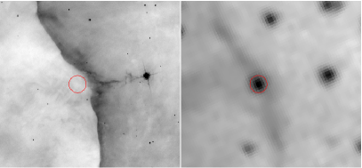
Figure 2: HH903 is clearly visible in the HST H$\upalpha$ image (left), but no source for the jet is visible. In the Spitzer 4.5 $\upmu\mathrm{m}$ image (right), a point-like source (red circle) is revealed that is very likely the source of jet emission. The circle marking the source has a radius of 2″.

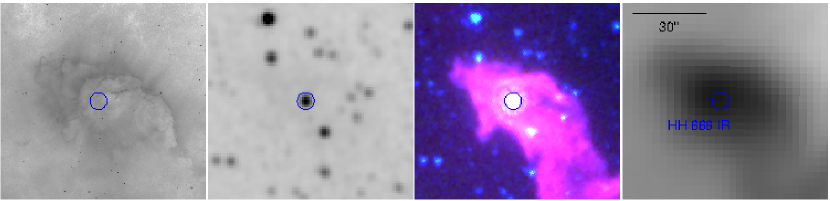
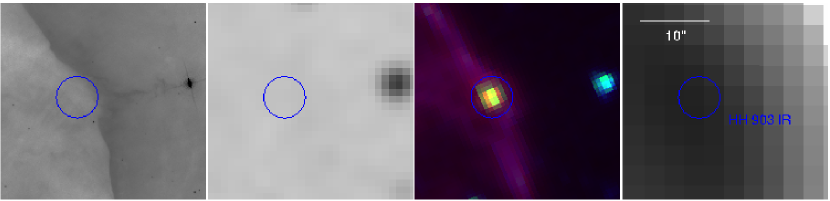
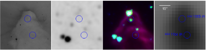
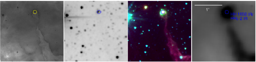
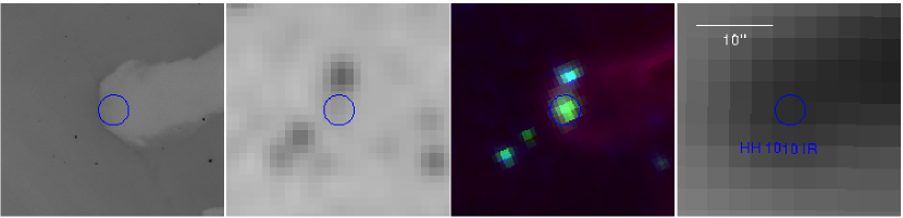
Figure 3: The Herbig-Haro jets and Herbig-Haro jet candidates in four different wavelengths. Each row represents from left to right the Hubble Space Telescope H$\upalpha$ (Ford & ACS Science Team 2000, obtained via the Hubble Legacy Archive) image, the 2MASS K-band image (Skrutskie et al. 2006, obtained via the NASA/IPAC Infrared Science Archive), a Spitzer RGB image with 3.6 $\upmu\mathrm{m}$ in blue, 4.5 $\upmu\mathrm{m}$ in green and 8.0 $\upmu\mathrm{m}$ in red, and Herschel 170 $\upmu\mathrm{m}$ in the rightmost panel. The sources marked with blue circles (partly yellow for better visibility) and labelled in the Herschel image are those sources of jet objects that are listed in Table 2. Spatial scale was chosen individually and is indicated separately for each row.

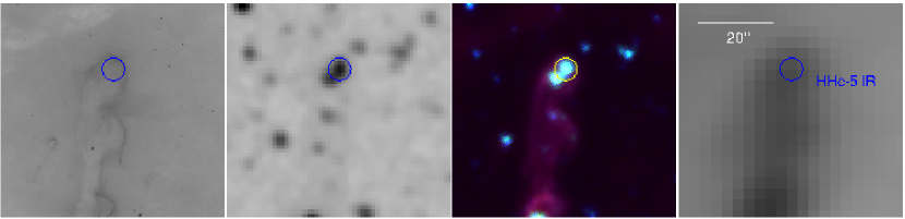
Figure 3: Continued.

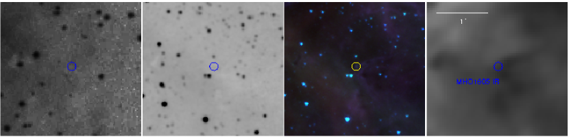
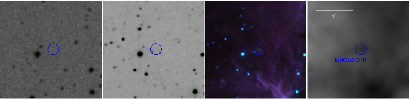
Figure 4: As in Fig. 3, but showing the two MHOs identified with Spitzer sources. Instead of the HST image, the leftmost image in each panel shows the STScI Digitized Sky Survey (DSS) optical image.

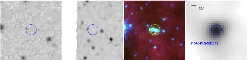
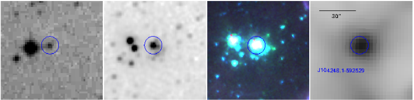
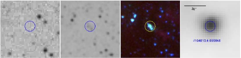
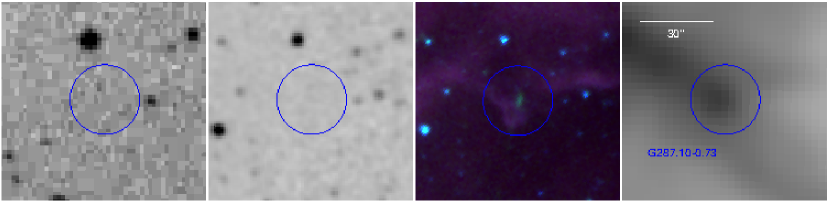
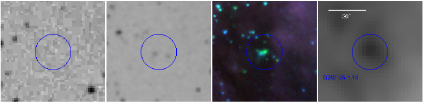
Figure 5: As Fig. 4, but showing the seven EGOs in our jet source sample.

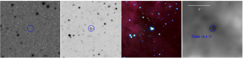
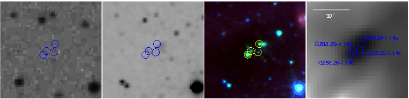
Figure 5: Continued.

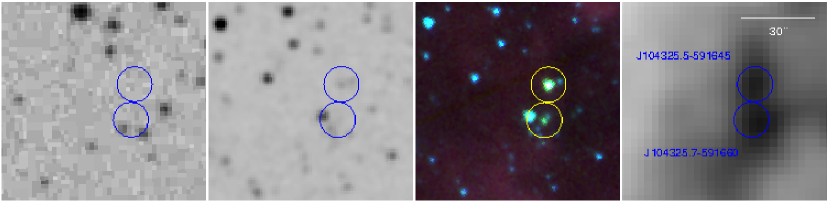
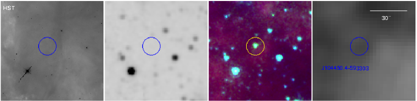
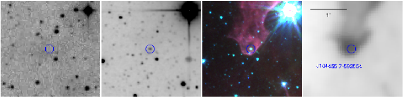
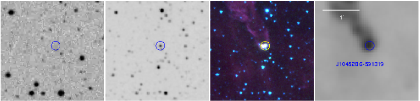
Figure 6: As Fig. 4, showing the five CGOs in our sample. The leftmost image in each panel is the HST image instead of DSS if indicated by an “HST” in the upper left-hand corner.

3.1 The search for sources of the Herbig-Haro jets

The mosaic images created from Spitzer data as described above were then submitted to visual inspection for probable sources of the 20 Herbig-Haro objects and 15 Herbig-Haro candidates within our field as identified from HST H$\upalpha$ images by Smith et al. (2010a). For 22 HH objects and HH candidates of these 35 objects in our sample, we were able to identify a Spitzer point-like source that constitutes a probable jet source, lying on the jet axis or on its projection. Eight of them could also be identified with a point-like Herschel source. (Two jets were identified with the same source; see 3.1.3.) In one case, that of HH 900, a Herschel source is seen but is probably not associated with a protostar, but rather with the surrounding globule. The remaining twelve jets have neither Spitzer nor Herschel sources that correspond with them. Some outstanding cases are described below.

3.1.1 HH 666

The jet HH 666 emanates from out of a pillarhead. This object has already been the subject of a detailed analysis in the infrared by Smith et al. (2004). Prominent in this pillarhead is a very bright Spitzer source, which we identified as the source of the jet. It is also associated with a clear point-like Herschel source. For the SED fit we added the optical and near-IR fluxes as published by Smith et al. (2004) to our Spitzer and Herschel fluxes.

3.1.2 HH 1004 and HH 1005

Both the jets assigned as HH 1004 and HH 1005 by Smith et al. (2010a) are located towards the tip of the same pillar. Two of the several sources located within this pillar seem to be likely sources for them. The lower part of the clearly two-part structure that is HH 1004 is in line with a faint Spitzer point-like source that is associated with a distinct compact Herschel source and a HAWK-I point-like source. A second Herschel source towards the north of it is coincident with a brighter Spitzer source and might be a likely source for the jet HH 1005.

3.1.3 HH 1008 and HH c-2

HH c-2 is placed right at the top of a thin, elongated pillar, with a very bright Spitzer source and a distinct Herschel counterpart located inside the pillar head, coincident with a 2MASS point-like source. HH 1008 is bow-shaped and placed to the south-east of the same pillar head. It is probable that it was caused by the same bright source, since it is well aligned with it, and there is no other candidate source in the vicinity.

3.1.4 HH c-10

HH c-10 is a bow-like structure and, like HH 1008, might have been caused by a source in the nearby head of the pillar close to which it is located. Within this pillarhead, however, there are three distinct Spitzer sources while no definite Herschel detection can be made. Thus, it remains unclear which, if any, of the Spitzer objects might be the source of the Herbig-Haro candidate.

3.2 The search for sources of the Molecular Hydrogen Emission Objects

A very similar process was applied to the MHOs detected in Preibisch et al. (2011b) which were subjected to visual inspection to search for probable Spitzer point-like sources. Four of the six MHOs are located in regions that are comparatively free of Spitzer-detected point-like sources and show no Spitzer counterparts themselves. Two of them, MHOs 1605 and 1610, however, show a counterpart within the source catalogue. These are the two objects from the sample of six that are located towards the edge of a pillar or globule, both close to or within known clusters (Tr 14 and 16).

The HAWK-I data cover only a subfield of the one surveyed in this work, so there might be other H${}_{\mbox{2}}$ sources that could not be detected. For the region surveyed with HAWK-I, since all peculiar features in H${}_{\mbox{2}}$ emission were described in the study in Preibisch et al. (2011b), no further coincidental detections can be reported.

3.3 The search for extended green objects and compact green objects

Successively, in the IRAC images we also visually searched for sources with excessive 4.5 $\upmu\mathrm{m}$-band emission, either extended (EGOs) or point-like (CGOs). The RGB images (3.6 $\upmu\mathrm{m}$ in blue, 4.5 $\upmu\mathrm{m}$ in green and 8.0 $\upmu\mathrm{m}$ in red) were scaled freely to obtain the best possible visibility of unusually green objects. However, De Buizer & Vacca (2010) make the valid point that to be able to identify EGOs, the 4.5 $\upmu\mathrm{m}$ band usually needs to be scaled up unproportionally high with regard to the red and blue bands. Thus, the weaker emission on the flanks of a relatively extended, bright source might appear to be green only because the scaling was chosen in this way. This is a caveat to be kept in mind when dealing with EGOs surrounding regular point-like sources. Since our EGOs are all well away from bright point-like sources, it is still possible excessively high scaling of the 3.6 $\upmu\mathrm{m}$ band caused them to appear, but care was taken to make sure they were real phenomena.

Care was also taken to check whether especially CGOs were not simply imaging faults and green excess was not caused by faulty pixels in the other bands. It can, however, not be excluded that a minority of the peculiarly CGOs are seen for those reasons and are not real objects. They were selected by visually scanning the processed Spitzer images for sources that appeared to the eye to have an excess in the 4.5 $\upmu\mathrm{m}$ (green) band compared to their immediate surroundings. Overall, we found three EGOs and five CGOs within the studied area (Fig. 5).

3.3.1 EGOs

All three new EGOs can clearly be identified with a compact Herschel counterpart. Though by nature they are extended, for all three of them we can identify a probable Spitzer source for which photometry could be obtained. One of them, J104248.1-592529, is also coincident with a 2MASS source, which allowed for photometry in another three bands.

In addition to the three newly discovered objects we included in our study the four EGOs within the CNC identified by Smith et al. (2010b). They were subjected to the same analysis as the objects identified through the processes described above. The object described by Smith et al. as G288.26-1.14 appears to be a multiple object. It was therefore split into four objects marked a to d for the analysis. Smith et al. (2010b) note the multiplicity and point out that some of the green objects in this cluster might not be true EGOs, they should thus be treated with caution. Only for the object designated G288.26-1.14a a compact Herschel source is seen, for the other three components no Herschel fluxes could be derived.

Likewise, G288.15-1.17 is a composite object. In the Spitzer image, it can be recognised as consisting of at least three separate sources (cf. Fig. 5), which is also true for the 2MASS image. Thus, though we could identify Spitzer sources and also a corresponding compact Herschel object, we did not use the photometry for SED fitting, since it would be highly likely to be comprised of different sources.

For the other two objects we were each able to identify a compact Herschel counterpart.

3.3.2 Compact green objects

It is the very nature of compact green objects to be identified with a single Spitzer source. Four of them also show a compact Herschel counterpart. One, J104450.4-593303, is within a region of diffuse Herschel emission, but this is not point-like and could thus not be employed for photometry. For J104528.6-591319, a 2MASS source could be identified and photometry employed for the fitting process.

4 Characteristics of jet sources

4.1 Radiative transfer modelling of the SEDs

From the collected data at Spitzer and Herschel wavelengths, we consecutively constructed SEDs for the four Spitzer IRAC and five Herschel PACS and SPIRE wavelengths, complemented by the LABOCA, HAWK-I, and 2MASS fluxes, as far as photometry was available for the respective sources. For SED-fitting we used the online tool of Robitaille et al. (2007). This tool compares the input observational data with 200 000 SED models for YSOs that were precomputed using a 2D radiative transfer code by Whitney et al. (2003). These models have a wide parameter space for the properties of the central object and its environment. The important parameters for our study are stellar mass, circumstellar disk mass, envelope mass, and total luminosity. Because our data sample the peak of the protostar’s SED, they give a good constraint on its total luminosity.

Herschel, Spitzer, and LABOCA fluxes as listed in Table 2, complemented by HAWK-I and 2MASS fluxes where available, were used for the compilation of the SEDs. No fits were performed for sources with only Spitzer fluxes or fewer than four data points overall because no reasonable constraints to the model could be obtained in these cases. For the fits, the distance to all objects was assumed to be 2.3 kpc, and the interstellar extinction range was restricted to to $A_{V}=0\dots 40$ mag. We assumed an uncertainty of 20% for all fluxes. In addition to the best-fit model, we show the range of possible parameters that can be derived from models within the range of $\chi^{2}\!/\nu-\chi_{\mathrm{best}}^{2}/\nu<2$ (with $\nu$ representing the number of data points). These models are shown as grey lines in the plots in Fig. 7. The resulting model parameters are listed in Table 3. It gives the best-fit value together with the range constrained by the above $\chi^{2}$ criterion. The resulting SEDs are shown in Fig. 7.

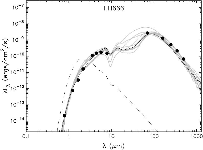
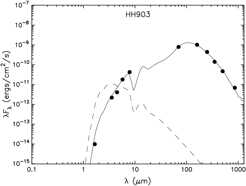
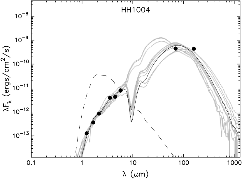
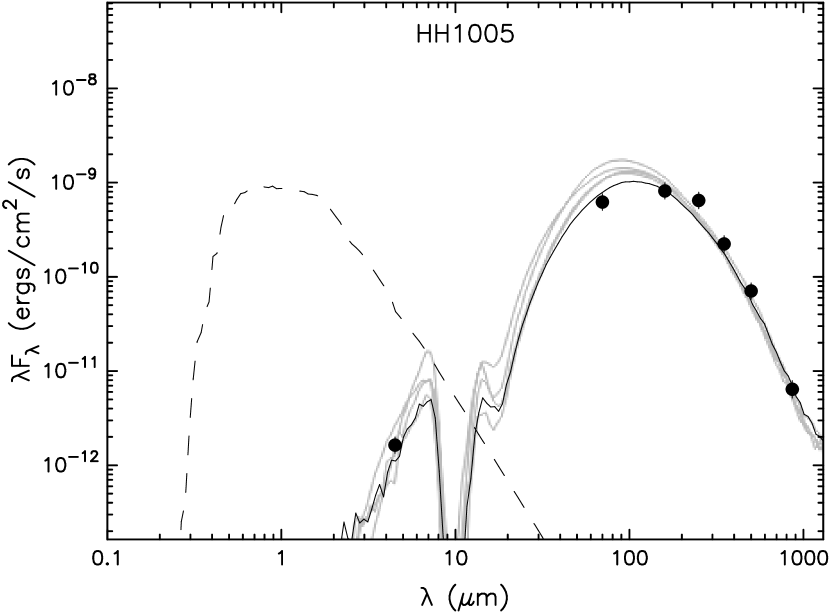
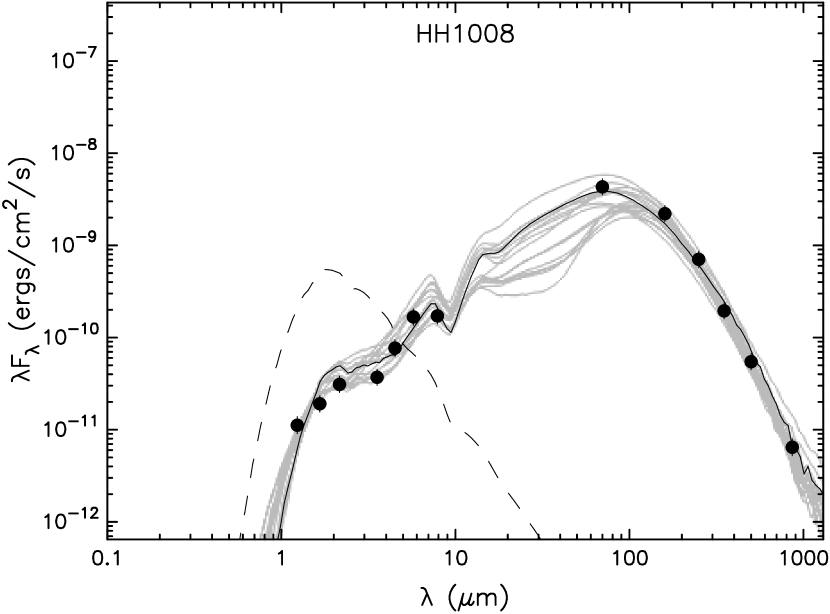
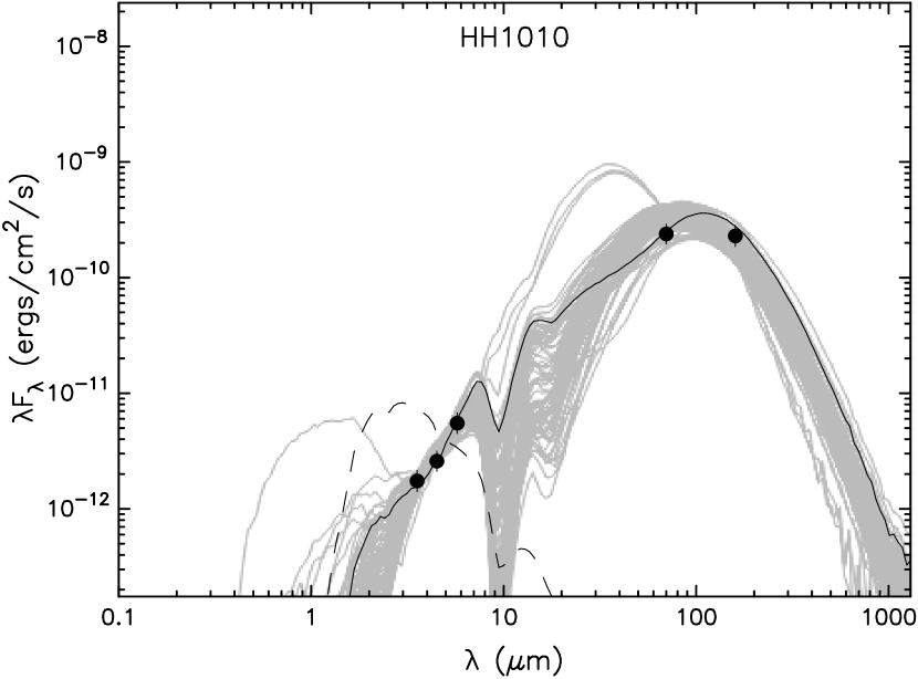
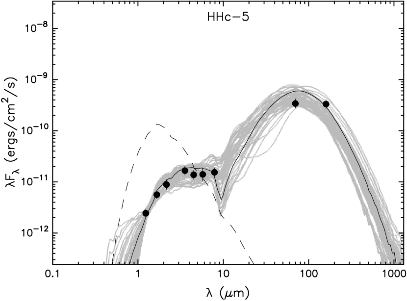
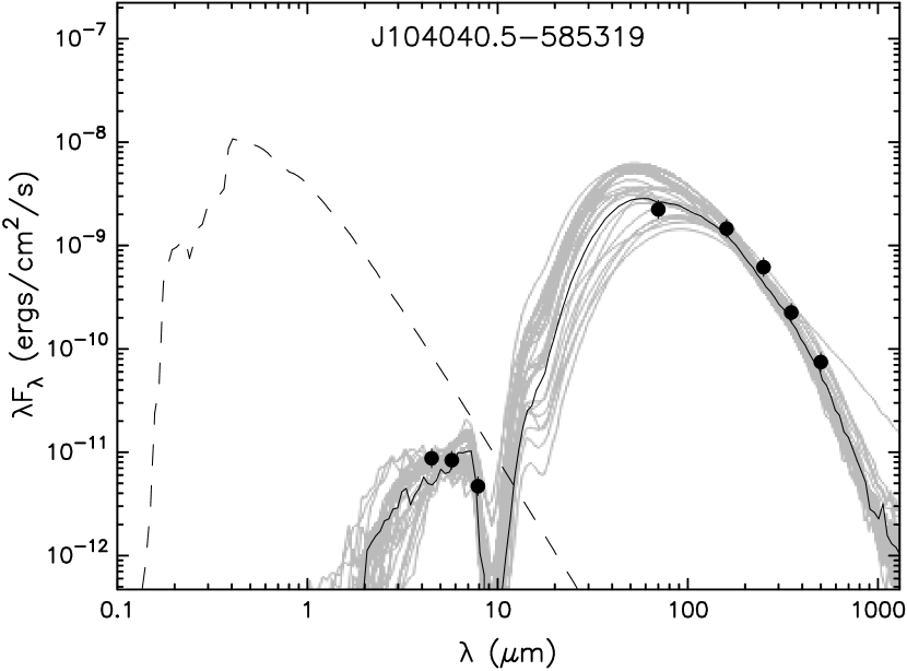
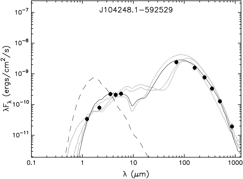
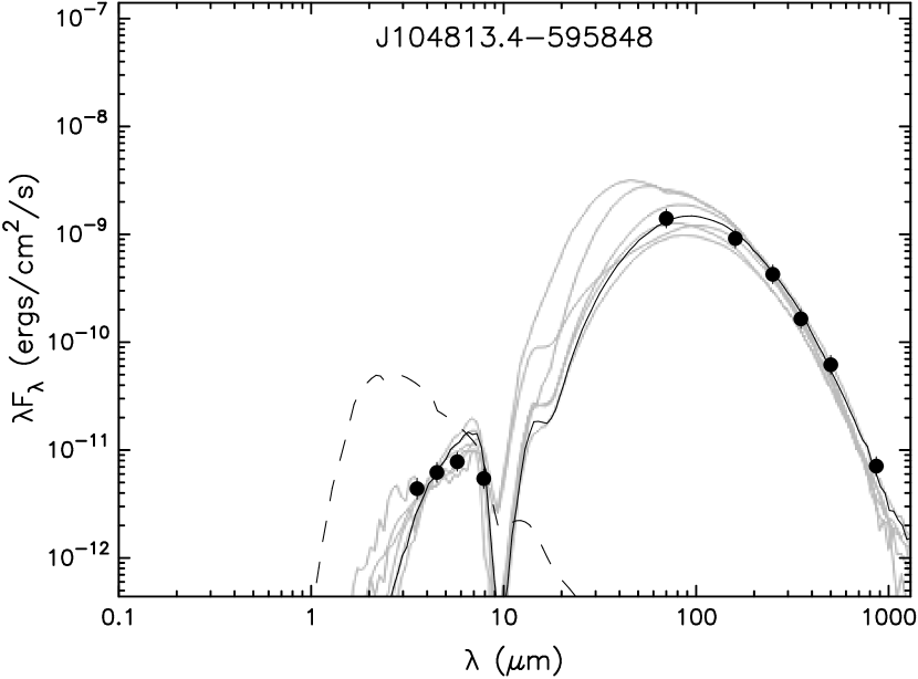
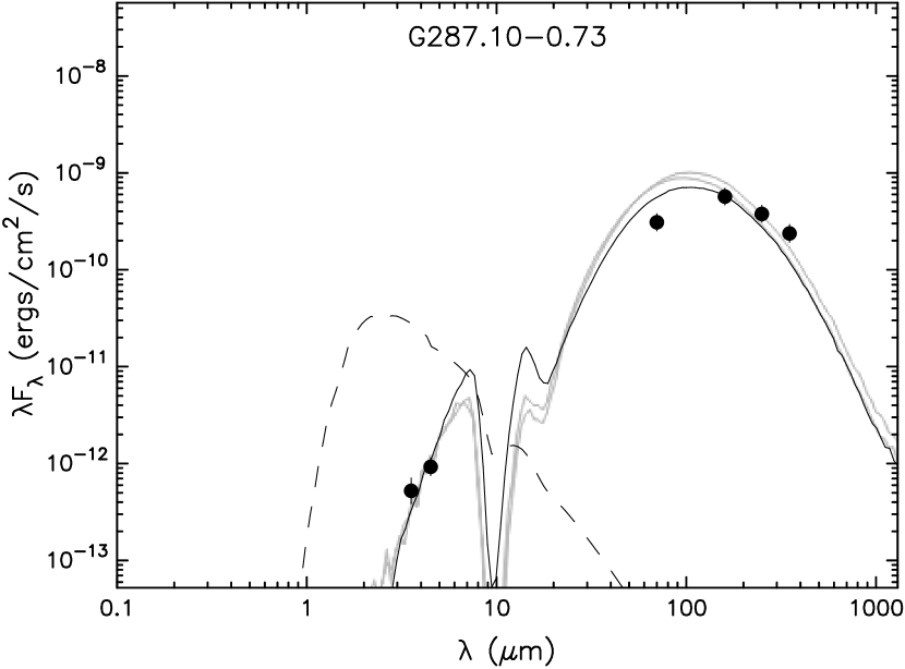
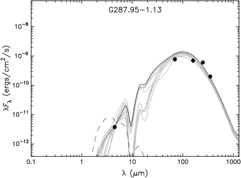
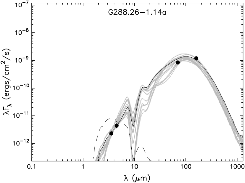
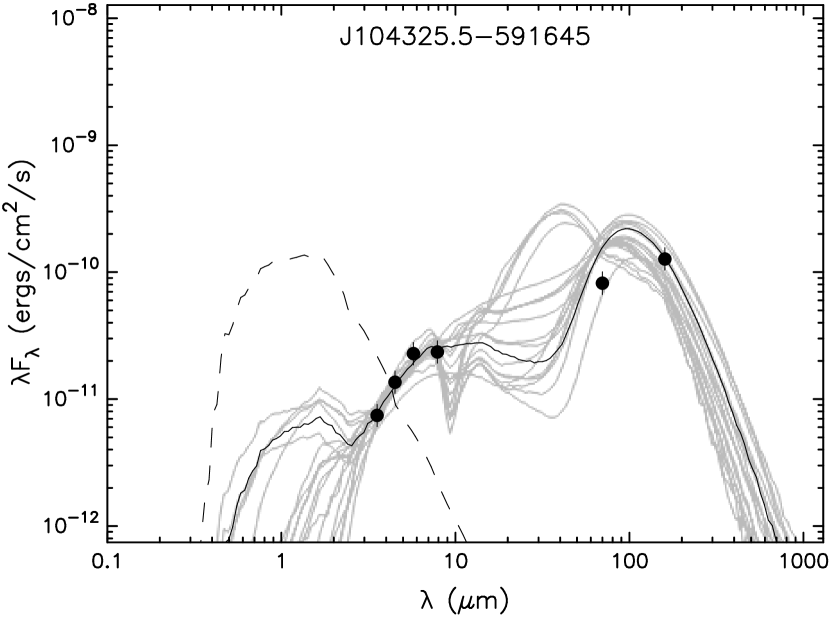
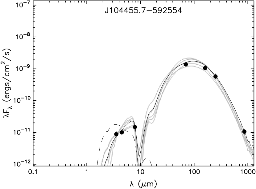
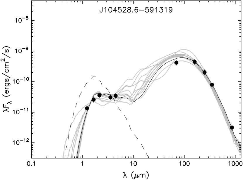
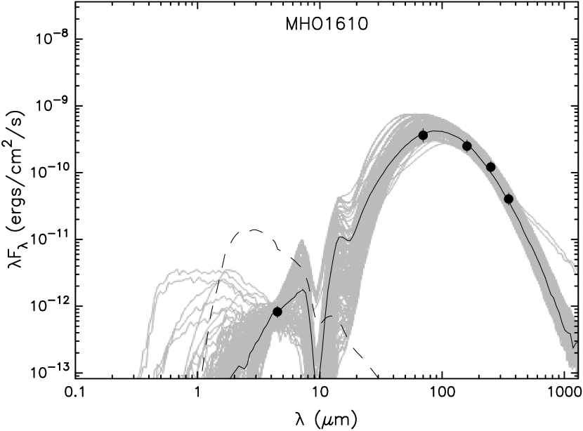
Figure 7: Spectral energy distributions of those 17 objects for which we could determine fluxes in at least four bands overall. Filled circles mark the input fluxes. The black line shows the best fit, and the grey lines show subsequent good fits. The dashed line represents the stellar photosphere corresponding to the central source of the best-fitting model, as it would appear in the absence of circumstellar dust (but including interstellar extinction).

Notably, all the sources in our sample are well modelled by models possessing a circumstellar disk. The masses of the jet-emitting protostars are within a range of $\leavevmode\nobreak\ 1-10\,M_{\odot}$. Thus, they all are of low masses, with luminosities of the best-fit models varying between 40 and $1600\,L_{\odot}$. Most of the luminosities are in the lower range below a few hundred $L_{\odot}$, with three notable exceptions that exhibit luminosities of more than $700\,L_{\odot}$. Sources of CGOs seem to be lower-mass (best-fit values $\sim 1-5\,M_{\odot}$) than those of EGOs (best-fit values $\sim 5-8\,M_{\odot}$), while those objects emitting HH jets are of varying masses (best-fit values $\sim 2-7\,M_{\odot}$). Envelope masses of EGO sources are noticeably higher than most of those for other jet objects. All best-fit envelope masses for EGO sources are at least $350\,M_{\odot}$, while many of those for the other objects (6 out of 11, 55%) are far below $100\,M_{\odot}$. However, five of those also range far above that value. There is no distinct pattern recognisable for the disk masses, if any, that HH jet sources have slightly higher disk masses than those of the other jet objects. Still, the smallness of the sample means that these observations of course only have limited statistical value. For MHOs especially, we only have a single specimen so that no qualitative statements are possible.

Table 2: Source fluxes as obtained in the Spitzer (3.6 $\upmu\mathrm{m}$, 4.5 $\upmu\mathrm{m}$, 5.8 $\upmu\mathrm{m}$, and 8.0 $\upmu\mathrm{m}$) and Herschel (70 $\upmu\mathrm{m}$, 160 $\upmu\mathrm{m}$, 250 $\upmu\mathrm{m}$, 350 $\upmu\mathrm{m}$, and 500 $\upmu\mathrm{m}$) bands, complemented with LABOCA 870 $\upmu\mathrm{m}$ photometry and JHK${}_{\mbox{s}}$ photometry as obtained with HAWK-I or from the 2MASS point-source catalogue.

Jet Source		3.6 $\upmu\mathrm{m}$	4.5 $\upmu\mathrm{m}$	5.8 $\upmu\mathrm{m}$	8.0 $\upmu\mathrm{m}$	70 $\upmu\mathrm{m}$	160 $\upmu\mathrm{m}$	250 $\upmu\mathrm{m}$	350 $\upmu\mathrm{m}$	500 $\upmu\mathrm{m}$	870 $\upmu\mathrm{m}$	J	H	K${}_{\mbox{s}}$
		[mJy]	[mJy]	[mJy]	[mJy]	[Jy]	[Jy]	[Jy]	[Jy]	[Jy]	[Jy]	[mJy]	[mJy]	[mJy]
HH666 IR	J104351.5–595521	137	238	338	405	64.6	70.5	43.9	25.6	11.4	–	0.33	1.9	12
HH902 IR	J104401.8–593030	–	4.17	29.6	70.0	–	–	–	–	–	–	–	–	–
HH903 IR	J104556.4–600608	2.68	6.24	35.4	115	19.1	55.7	37.9	16.7	8.07	2.03	–	–	–
HH1004 IR	J104644.8–601021	4.75	6.58	15.2	–	10.6	23.9	–	–	–	–	0.0540	0.206	0.624
HH1005 IR	J104644.2–601035	–	2.50	–	–	14.8	44.4	55.0	26.6	12.0	1.89	–	–	–
HH1006 IR	J104632.9–600354	2.57	3.06	10.6	23.1	–	–	–	–	–	–	–	–	–
HH1008/c-2 IR	J104445.4–595555	44.8	117	326	461	103	120	59.9	23.2	9.32	1.90	4.71	10.8	22.8
HH1010 IR	J104148.7–594338	2.11	3.96	10.8	–	5.67	12.5	–	–	–	–	–	–	–
HH1012 IR	J104438.7–593008	5.29	5.27	5.92	–	–	–	–	–	–	–	–	–	–
HH1013 IR	J104419.2–592612	8.46	11.7	16.7	25.1	–	–	–	–	–	–	–	–	–
HH1017 IR	J104441.5–593357	4.98	5.12	–	–	–	–	–	–	–	–	–	–	–
HH1018 IR	J104452.9–594526	4.54	5.39	–	10.5	–	–	–	–	–	–	–	–	–
HHc-1 IR	J104405.4–592941	6.00	–	–	–	–	–	–	–	–	–	–	–	–
HHc-3 IR	J104504.6–600303	0.611	0.712	2.34	5.02	–	–	–	–	–	–	–	–	–
HHc-5 IR	J104509.4–600203	20.0	21.1	27.9	41.2	8.12	18.1	–	–	–	–	1.02	3.17	6.52
HHc-6 IR	J104509.2–600220	–	1.29	–	–	–	–	–	–	–	–	–	–	–
HHc-7 IR	J104513.0–600259	2.25	2.00	–	–	–	–	–	–	–	–	–	–	–
HHc-8 IR	J104512.0–600310	5.48	8.33	13.2	16.0	–	–	–	–	–	–	–	–	–
HHc-13 IR	J104400.6–595427	13.2	12.5	13.8	17.1	–	–	–	–	–	–	–	–	–
HHc-15 IR	J104353.9–593245	274	285	283	239	–	–	–	–	–	–	–	–	–
EGO	J104040.5–585319	–	13.4	16.3	12.6	53.2	79.4	52.7	26.8	12.7	–	–	–	–
EGO	J104248.1–592529	265	318	440	–	57.3	85.9	65.4	39.4	21.8	5.73	14.0	–	58.1
EGO	J104813.4–595848	5.34	9.52	15.2	14.6	33.4	49.8	36.2	19.6	10.5	2.09	–	–	–
G287.10-0.73	J104114.3–593239	0.645	1.42	–	–	7.36	31.0	32.2	28.3	–	–	–	–	–
G287.95-1.13	J104542.0–601732	–	5.80	–	–	18.4	38.2	51.0	23.8	–	–	–	–	–
G288.26-1.14a	J104750.3–602618	2.83	6.70	–	–	20.0	65.0	–	–	–	–	–	–	–
G288.26-1.14b	J104752.1–602627	4.02	14.5	28.8	31.3	–	–	–	–	–	–	–	–	–
G288.26-1.14c	J104750.9–602625	1.13	1.93	–	–	–	–	–	–	-	–	–	–	–
G288.26-1.14d	J104751.7–602624	2.25	–	–	–	–	–	–	–	–	–	–	–	–
CGO	J104325.5–591645	8.99	20.8	44.5	63.0	1.95	6.93	–	–	–	–	–	–	–
CGO	J104325.7–591660	1.60	3.26	6.69	8.22	–	–	10.5	7.10	4.78	–	–	–	–
CGO	J104450.4–593303	3.18	21.3	9.17	12.0	–	–	–	–	–	–	–	–	–
CGO	J104455.7–592554	10.6	15.4	–	39.6	32.7	57.4	48.8	–	–	3.11	0.821	1.64	2.75
CGO	J104528.6–591319	37.1	52.7	–	–	9.96	24.1	17.2	9.46	–	0.923	5.63	14.6	26.1
MHO1605 IR	J104351.5–593911	1.27	1.79	8.19	17.9	–	–	–	–	–	–	–	–	–
MHO1610 IR	J104608.3–594525	–	1.26	–	–	8.68	13.6	10.3	4.80	–	–	–	–	–

Table 3: Model parameters for the jet sources as obtained from the Robitaille et al. (2007) models.

Jet Source	Stellar Mass		Disk Mass		Envelope Mass		Total Luminosity		Best-Fit
	$[M_{\odot}]$		$[M_{\odot}]$		$[M_{\odot}]$		$[L_{\odot}]$		Model
J104351.5–595521	3.2	[1.7 – 9.2]	1.26$\cdot 10^{-1}$	[1.93$\cdot 10^{-2}$ – 5.68$\cdot 10^{-1}$]	20	[5.3 – 410]	420	[390 – 1400]	3014036
J104556.4–600608	4.3	[4.3 – 4.3]	1.74$\cdot 10^{-2}$	[1.74$\cdot 10^{-2}$ – 1.74$\cdot 10^{-2}$]	490	[490 – 490]	250	[250 – 250]	3018560
J104644.8–601021	4.6	[2.6 – 7.0]	1.40$\cdot 10^{-2}$	[7.32$\cdot 10^{-3}$ – 2.26$\cdot 10^{-1}$]	20	[4.9 – 250]	150	[81 – 1600]	3016324
J104644.2–601035	5.5	[5.5 – 7.3]	2.07$\cdot 10^{-1}$	[4.25$\cdot 10^{-3}$ – 5.87$\cdot 10^{-1}$]	760	[480 – 760]	230	[230 – 440]	3013239
J104445.4–595555	7.0	[2.1 – 8.1]	1.30$\cdot 10^{-1}$	[1.60$\cdot 10^{-3}$ – 3.42$\cdot 10^{-1}$]	560	[ 94 – 640]	710	[370 – 1000]	3006553
J104148.7–594338	1.9	[1.3 – 6.7]	2.08$\cdot 10^{-2}$	[7.76$\cdot 10^{-4}$ – 2.80$\cdot 10^{-1}$]	77	[6.1 – 250]	64	[40 – 1400]	3008354
J104509.4–600203	4.3	[1.4 – 6.4]	4.79$\cdot 10^{-3}$	[2.10$\cdot 10^{-4}$ – 2.73$\cdot 10^{-1}$]	43	[3.9 – 350]	130	[56 – 310]	3019527
J104040.5–585319	8.3	[1.9 – 10 ]	1.81$\cdot 10^{-2}$	[2.73$\cdot 10^{-3}$ – 6.71$\cdot 10^{-1}$]	350	[ 39 – 1300]	1700	[300 – 3400]	3002514
J104248.1–592529	8.1	[5.0 – 8.3]	7.32$\cdot 10^{-3}$	[7.32$\cdot 10^{-3}$ – 5.06$\cdot 10^{-1}$]	1500	[200 – 1700]	820	[460 – 1000]	3006025
J104813.4–595848	6.6	[3.6 – 8.3]	5.87$\cdot 10^{-1}$	[2.77$\cdot 10^{-3}$ – 5.87$\cdot 10^{-1}$]	550	[250 – 750]	330	[220 – 2500]	3013941
J104114.3–593239	6.5	[5.5 – 6.5]	1.91$\cdot 10^{-3}$	[1.91$\cdot 10^{-3}$ – 2.07$\cdot 10^{-1}$]	430	[430 – 760]	250	[230 – 250]	3020073
J104542.0–601732	4.9	[3.0 – 7.3]	7.72$\cdot 10^{-2}$	[2.77$\cdot 10^{-3}$ – 5.87$\cdot 10^{-1}$]	540	[300 – 550]	250	[190 – 420]	3014735
J104750.3–602618	4.9	[3.0 – 6.6]	7.72$\cdot 10^{-2}$	[2.77$\cdot 10^{-3}$ – 5.87$\cdot 10^{-1}$]	540	[ 66 – 550]	250	[190 – 380]	3014735
J104325.5–591645	1.3	[0.8 – 5.7]	9.63$\cdot 10^{-3}$	[6.35$\cdot 10^{-5}$ – 1.86$\cdot 10^{-1}$]	10	[1.9 – 53]	38	[23 – 760]	3002569
J104455.7–592554	4.6	[4.6 – 7.7]	8.23$\cdot 10^{-2}$	[4.79$\cdot 10^{-2}$ – 5.87$\cdot 10^{-1}$]	1200	[550 – 1200]	310	[230 – 570]	3000552
J104528.6–591319	2.6	[1.5 – 4.8]	4.25$\cdot 10^{-2}$	[1.05$\cdot 10^{-3}$ – 2.16$\cdot 10^{-1}$]	270	[ 65 – 300]	100	[94 – 200]	3003259
J104608.3–594525	3.6	[1.4 – 6.4]	1.34$\cdot 10^{-3}$	[2.52$\cdot 10^{-4}$ – 2.71$\cdot 10^{-1}$]	80	[9.3 – 250]	110	[52 – 260]	3004022

5 Discussion

We surveyed 55 jet objects and found corresponding point-like sources for 36 of them. For three of the CGOs and seven of the EGOs we were able to derive the SEDs of newly identified IR sources. Out of 35 HH jets and HH jet candidates, we could identify sources for 22 of them and model SEDs for seven. Out of the six MHOs within the HAWK-I field – which is smaller than the entire field surveyed here – we could only identify sources for two and find an SED model for one.

It is important to note that this study is not able to identify all the jet objects in the CNC. The majority of jets are just too faint and fall below the sensitivity limits of our data. Consequently, out of the members of the CNC that are currently undergoing jet-emitting phases, we can only observe a low percentage of the most luminous ones. This explains why out of the very large number of young stars within the surveyed region only so few jets are detected.

The stellar-mass estimates derived from SED fitting are in the range $\sim 1\,M_{\odot}$ to $\sim 10\,M_{\odot}$. This range agrees very well with the expectations in the following sense: The lower mass limit of $\sim 1\,M_{\odot}$ is probably a consequence of the detection limit. Although the Spitzer images are deep enough to detect stars below this mass limit, one has to keep in mind that it is necessary to detect emission from the jet, too. That the mass flow rates of jets and outflows from YSOs are roughly correlated to the stellar luminosity (and thus also to the stellar mass; e. g. Reipurth & Bally 2001) explains why we do not detect jets from YSOs of lower masses. The upper mass limit is more interesting, since there is no reason why the jets from high-mass protostars should not be observable, if such jets were present. The absence of jet-driving high-mass ($M\ga 20\,M_{\odot}$) protostars therefore suggests that no such objects are present. This agrees with the conclusion derived from the analysis of the sub-mm data of the cloud structure by Preibisch et al. (2011c) that the clouds present today in the Carina Nebula are not dense and massive enough for high-mass star formation. This suggests that the currently ongoing star formation process in the CNC is qualitatively different from the processes that led to the formation of dozens of very high-mass stars ($M\ga 50\,M_{\odot}$, e. g. Smith 2006) in the CNC a few million years ago.

Further conclusions about the star-formation process can be drawn from the properties of the jets and the jet-driving protostars. The first interesting result is found by comparing the number of jets detected in the infrared images to the number of HH jets detected in the optical HST images. For a quantitative analysis, we consider the $\approx 1.0\degr\times 1.3\degr$ region investigated by Smith et al. (2010a, their Fig. 1). Their (mostly non-contiguous) HST pointings cover $\approx 15\%$ of this area and have led to the detection of 34 HH jets and jet-candidates. If the full area had been observed by HST, the number of detected jets in this area would very likely be larger, perhaps $\sim 70$.

The number of jets detected in the infrared images of the same area is 20 (9 EGOs, 5 CGO, and 6 MHOs), i. e. substantially smaller. We are confident that this is not an effect of the cloud extinction, because the sub-mm observations (Preibisch et al. 2011c) have shown that the column densities and the extinction of almost all clouds in the region are rather low, generally $A_{V}\la 15$ mags. The clouds are therefore largely transparent for light in the Spitzer bands, so that we do not expect to miss a significant number of jets due to cloud extinction.

For comparing the number of optical HH jets to the infrared jets one has to keep in mind that these two groups are intrinsically different: The optical HH objects trace jets moving in the atomic gas outside the molecular clouds and originate in protostars located close to the surfaces of clouds. The infrared jets, on the other hand, trace molecular material inside the clouds (e. g. Elias 1980). Since almost all clouds should be essentially transparent at Spitzer wavelengths, one expects to see considerably more infrared jets than optical jets, assuming that the jet-driving sources are distributed in a spatially homogeneous way throughout the entire volume of the clouds. In many observations of nearby star-forming clouds, this expectation is confirmed (see e. g. Gutermuth et al. 2008, for the case of the NGC 1333 cloud).

In the case of the CNC, however, we see the opposite trend, i. e. the number of infrared jets is smaller than the number of optical jets. This suggests that most jet-driving protostars are located at the surfaces of the clouds, rather than in the inner cloud regions.

6 Conclusions

Our search for jets in wide-field Spitzer IRAC mosaic images of the CNC led to the detection of three new EGOs and five CGOs in and immediately around the area studied previously with the HST by Smith et al. (2010a). We also identified sources for 23 of the 34 HH jets in this area. Combining Spitzer and Herschel photometry with complementary LABOCA and HAWK-I/2MASS data, we obtained the spectral energy distributions of the jet sources through radiative transfer modelling (Robitaille et al. 2006, 2007) to estimate basic stellar and circumstellar parameters for 17 sources overall, where photometry in at least four bands could be obtained.

We find that the jet-driving protostars generally have low to intermediate masses ($\sim 1-10\,M_{\odot}$), which corroborates the notion that there is no current formation of high-mass stars in the CNC and that the present star formation epoch is thus different from the epoch that formed the present $\sim 70$ high-mass stars in Carina (Preibisch et al. 2011c). More optical jets, which come from sources close to the cloud surfaces, than IR jets from more deeply embedded sources, are seen in the region, showing that presently forming stars predominantly lie near the surfaces of clouds.