The intergalactic medium thermal history at redshift $z=1.7$–$3.2$ from the Ly-$\alpha$ forest: a comparison of measurements using wavelets and the flux distribution

Abstract

We investigate the thermal history of the intergalactic medium (IGM) in the redshift interval $z=1.7$–$3.2$ by studying the small-scale fluctuations in the Lyman-$\alpha$ forest transmitted flux. We apply a wavelet filtering technique to eighteen high resolution quasar spectra obtained with the Ultraviolet and Visual Echelle Spectrograph (UVES), and compare these data to synthetic spectra drawn from a suite of hydrodynamical simulations in which the IGM thermal state and cosmological parameters are varied. From the wavelet analysis we obtain estimates of the IGM thermal state that are in good agreement with other recent, independent wavelet-based measurements. We also perform a reanalysis of the same data set using the Lyman-$\alpha$ forest flux probability distribution function (PDF), which has previously been used to measure the IGM temperature-density relation. This provides an important consistency test for measurements of the IGM thermal state, as it enables a direct comparison of the constraints obtained using these two different methodologies. We find the constraints obtained from wavelets and the flux PDF are formally consistent with each other, although in agreement with previous studies, the flux PDF constraints favour an isothermal or inverted IGM temperature-density relation. We also perform a joint analysis by combining our wavelet and flux PDF measurements, constraining the IGM thermal state at $z=2.1$ to have a temperature at mean density of $T_{0}/[10^{3}$ K$]=17.3\pm 1.9$ and a power-law temperature-density relation exponent $\gamma=1.1\pm 0.1$ (1$\sigma$). Our results are consistent with previous observations that indicate there may be additional sources of heating in the IGM at $z<4$.

1 Introduction

The intergalactic medium (IGM) is the largest reservoir of baryonic matter in the early Universe, and so gaining an understanding of its physical state and chemical composition is an important goal of modern cosmology. In the current picture for the evolution of the baryons, there are two reionisation events which turned the neutral gas in the IGM into an ionised medium. The first reionisation event is thought to be caused by hydrogen (and neutral helium) ionising radiation produced by early galaxies. The precise redshift of this reionisation event is not well constrained but it is thought to initiate at a redshift no later than $z=11$ (Larson et al. 2011) and end by $z\simeq 6$, which is when the Universe becomes transparent to redshifted Lyman-$\alpha$ photons from quasars (Becker et al., 2001; Fan et al., 2006). The second reionisation event is expected to instead be driven by quasars at lower redshifts, which produce a hard ionising spectrum that can reionise singly ionised helium by $z\sim 3$ (Madau et al., 1999; Furlanetto & Oh, 2008; McQuinn et al., 2009). Photo-heating during both of these reionisation events leaves a ‘footprint’ on the thermal state of the IGM; determining the redshift evolution of the IGM temperature can therefore help pin down the details of these reionisation eras (e.g. Theuns et al. 2002; Hui & Haiman 2003; Raskutti et al. 2012).

In the simplest picture, the competition between photo-heating and cooling due to the adiabatic expansion of the Universe results in a power-law temperature-density relation following reionisation, $T=T_{0}\Delta^{\gamma-1}$ for $\Delta={\rho}/{\langle\rho\rangle}<10$. The density dependence of the recombination rate means that higher density gas recombines faster, yielding more neutral atoms per unit time for photo-heating. These regions thus cool less rapidly than lower density gas, resulting in a temperature-density relation which evolves from isothermal ($\gamma\sim 1$) following reionisation toward a power-law with $\gamma\sim 1.6$ (Hui & Gnedin 1997). In principle, if the redshift dependence of the temperature-density relation can be measured then the timing of reionisation can thus be inferred. Indeed, by studying the thermal widths of absorption lines in the Lyman-$\alpha$ forest, Schaye et al. (2000) observed an increase in the temperature at mean density and a flattening of the temperature-density relation at $z\sim 3$, which may indicate the epoch of He$\,\rm\scriptstyle II\$reionisation occurred around this time.

However, this is a somewhat simplified picture; according to the numerical simulations presented by McQuinn et al. (2009), He$\,\rm\scriptstyle II\$reionisation is inhomogeneous and long-range heating by hard photons will induce large-scale fluctuations of the order of 50 comoving Mpc in the IGM temperature and He$\,\rm\scriptstyle II\$ionisation state. Another question mark hangs over the slope of the temperature-density relation describing the IGM thermal state. Observational work from Becker et al. (2007), Bolton et al. (2008) and Viel et al. (2009) has suggested that the IGM may obey an ‘inverted’ ($\gamma<1$) temperature-density relation in which, somewhat counter-intuitively, less dense gas is hotter than denser gas. Although it appears difficult to produce this result by He$\,\rm\scriptstyle II\$photo-heating by quasars (McQuinn et al. 2009; Bolton et al. 2009), it has recently been suggested by Chang et al. (2011) and Puchwein et al. (2011) that it could be a consequence of volumetric heating by TeV emission from blazars.

Given these uncertainties, it is important to investigate the observational constraints in more detail. One way to achieve this is to directly compare different methods used to measure the IGM thermal state. This allows one to establish whether these different approaches are consistent, or whether there are systematic uncertainties which impact differently upon the competing approaches. The methodologies used in the literature thus far to measure the IGM thermal state from the Lyman-$\alpha$ forest can be broadly divided in two classes. The common feature in both approaches is that they measure the IGM temperature via the impact of Jeans (pressure) smoothing and thermal Doppler broadening on the Lyman-$\alpha$ forest. The first class consists of methods that fit Voigt profiles to each absorption line in the Lyman-$\alpha$ forest. Examples of this class are the earlier work of Schaye et al. (2000), Ricotti et al. (2000) and McDonald et al. (2000) and more recently Bolton et al. (2010). The second class consists of methods in which the transmitted flux is analysed with a global statistical approach, without decomposing the spectra into separate features. Power spectra studies belong to this class (Zaldarriaga et al., 2001; Viel et al., 2009), as well as methods that examine other statistical properties of the forest, such as the flux probability distribution function (PDF) (Bolton et al., 2008; Calura et al., 2012), the wavelet analysis method applied in Lidz et al. (2010) and the ‘curvature’ statistic used by Becker et al. (2011).

The main aim of this work is to compare two of these competing techniques, the flux PDF and wavelets, by applying them to the metal-cleaned Lyman-$\alpha$ forest spectra presented by Kim et al. (2007). These data have previously been used in studies of the flux PDF which have found the IGM temperature-density relation may be isothermal or inverted at $2<z<3$ (Bolton et al. 2008; Viel et al. 2009). In order to interpret the results we have also utilised and extended the suite of hydrodynamical simulations used in the analysis of Becker et al. (2011). This comparison is of particular interest because, as pointed out by Lidz et al. (2010), there appears to be some tension between the IGM thermal parameters inferred from wavelets and the flux PDF, particularly with respect to measurements of the slope of the temperature-density relation. This paper is therefore organised as follows: in Section 2 we review the observations and numerical simulations used; in Section 3 our implementation of the wavelet analysis is presented; in Section 4 we describe our interpolation and parameter determination methodology and in Section 5 we present our results along with a comparison to previous studies. We conclude in Section 6. An appendix at the end of the paper lists the simulations we use in this study, along with several tests for numerical convergence and the sensitivity of our results to parameter assumptions.

2 Observations and numerical simulations

In this section we briefly review our observational dataset, the numerical simulations used for our theoretical interpretation and the procedure used to generate synthetic spectra.

2.1 Spectra, metal removal and continuum placement

Our analysis uses the eighteen metal-cleaned quasar spectra from Kim et al. (2007) obtained with the Ultraviolet and Visual Echelle Spectrograph (UVES) on the VLT. The spectra are sampled with pixels of width $0.05\mbox{\,}{\rm\AA}$ and have a signal to noise ratio per pixel of order $30\mbox{--}50$. In order to avoid the proximity effect, the region 4000 $\rm km\,s^{-1}$ bluewards of the Lyman-$\alpha$ emission line has been excluded. These spectra contain Lyman limit systems with column densities in the interval $10^{17.2}{\rm cm}^{-2}\leq N_{\rm HI}\leq 10^{19}{\rm cm}^{-2}$, but no damped Lyman-$\alpha$ systems, defined by a column density $N_{\rm HI}\geq 10^{20.3}{\rm cm}^{-2}$.

In order to correct the H$\,\rm\scriptstyle I\$absorption for metal contamination, metal absorption lines in the spectra were identified and fitted with Voigt profiles. These were substituted by a continuum level or by a Lyman-$\alpha$ only absorption profile generated from the fitted Lyman-$\alpha$ parameters (see Kim et al. 2007 for details). Note this approach differs from the metal removal procedure used in Lidz et al. (2010), where only narrow absorption lines (with $b<7\,{\rm km/s}$) were identified as metals and excised from the spectra.

The continuum level in the spectra was determined by locally connecting regions that are thought to be absorption-free. This is an iterative procedure, which starts with connecting non absorbed regions and is subsequently updated during the process of Voigt profile fitting the H$\,\rm\scriptstyle I\$and metal lines. Note that in our analysis we neglect the possibility of having an extended and slowly varying continuum absorption. This means that spectral regions which are considered to be absorption free could actually suffer from absorption by a broad H$\,\rm\scriptstyle I\$density fluctuation, and the measured optical depth would then be underestimated. We shall discuss the effect of continuum placement on our results further in Section 5.1.

QSO	$z_{\mathrm{em}}$	$z_{\mathrm{Ly\alpha}}$	$\lambda_{\mathrm{Ly\alpha}}(\rm{\mbox{\AA}})$	S/N
Q0055–269	3.655	2.936$-$3.205	4785$-$5112	80$-$50
PKS2126–158	3.279	2.815$-$3.205	4638$-$5112	50$-$200
Q0420–388	3.116	2.480$-$3.038	4231$-$4909	100$-$140
HE0940–1050	3.078	2.452$-$3.006	4197$-$4870	50$-$130
HE2347–4342	2.874	2.336$-$2.819	4055$-$4643	100$-$160
Q0002–422	2.767	2.209$-$2.705	3901$-$4504	60$-$70
PKS0329–255	2.704	2.138$-$2.651	3815$-$4439	30$-$55
Q0453–423	2.658	2.359$-$2.588	4084$-$4362	90$-$100
HE1347–2457	2.609	2.048$-$2.553	3705$-$4319	85$-$100
Q0329–385	2.434	1.902$-$2.377	3528$-$4105	50$-$55
HE2217–2818	2.413	1.886$-$2.365	3509$-$4091	65$-$120
Q0109–3518	2.405	1.905$-$2.348	3532$-$4070	60$-$80
HE1122–1648	2.404	1.891$-$2.358	3514$-$4082	70$-$170
J2233–606	2.250	1.756$-$2.197	3335$-$3886	30$-$50
PKS0237–23	2.223	1.765$-$2.179	3361$-$3865	75$-$110
PKS1448–232	2.219	1.719$-$2.175	3306$-$3860	30$-$90
Q0122–380	2.193	1.700$-$2.141	3282$-$3819	30$-$80
Q1101–264	2.141	1.880$-$2.097	3503$-$3765	80$-$110

Table 1: Properties of the quasar spectra from Kim et al. (2007). $z_{\mathrm{em}}$ is the approximate redshift of the quasar measured from the Lyman-$\alpha$ emission line; $z_{\mathrm{Ly\alpha}}$ and $\lambda_{\mathrm{Ly\alpha}}$ are the redshift and wavelength intervals associated with the Lyman-$\alpha$ absorption; S/N is the signal to noise ratio per 0.05Å pixel.

2.2 Numerical simulations

The simulations we use are based on the suite of models used by Becker et al. (2011), which we have extended by further varying the cosmological and IGM thermal parameters assumed. We make use of Gadget-3 code which is a parallel smoothed particle hydrodynamics code (Springel, 2005). Our simulations are performed in a periodic box of $10$ comoving Mpc$/h$ in linear size. We describe the evolution of both the dark matter and the gas, using $256^{3}$ particles for simulations in which the cosmological parameters are varied, or $2\times 512^{3}$ particles for simulations in which the IGM thermal state parameters are varied. A summary of the simulations is given in Tab 3 in the appendix.

The simulations all start at $z=99$ with initial conditions generated using the Eisenstein & Hu (1999) transfer function. Star formation is incorporated using a simplified prescription in which all gas particles with $\Delta>10^{3}$ and temperature $T<10^{5}$ K are converted into collisionless stars. Since we are not interested in the details of star formation, we thereby avoid the small dynamical times that would arise due to these overdense regions. As the bulk of the Lyman-$\alpha$ forest absorption corresponds to densities $\Delta<10$, this prescription has an impact at below the percent level on the final computation of flux PDF and flux power (Viel et al., 2004) and so we expect this will not affect our work. To check numerical convergence of our simulations we have also performed a series of simulations with varying gas particle and box size. We conclude from these tests, demonstrated in Figure 13 in the appendix, that our study of the statistics of small-scale structure of the Lyman-$\alpha$ forest demand the relatively high mass resolution afforded by a large number of particles, $2\times 512^{3}$, in a 10$h^{-1\,}$Mpc volume. With greater computational resources, we could improve the accuracy of our simulations by increasing the box size from 10 $h^{-1\,}$Mpc, while maintaining high mass resolution. However we believe that the possible improvements are small compared to the error budget we have assumed in Section 3.2.

A spatially uniform ultraviolet (UV) background applied in the optically thin limit determines the photo-heating and photo-ionisation of the gas in the simulations. In order to generate different thermal histories, we have rescaled all of the H$\,\rm\scriptstyle I\$, He$\,\rm\scriptstyle I\$and He$\,\rm\scriptstyle II\$photo-heating rates using the Haardt & Madau (2001) UV background model for galaxy and QSO emission. The photo-heating rates, $\epsilon_{\rm i}$, were changed by rescaling their values in a density dependent fashion, $\epsilon^{\rm new}_{\rm i}=\zeta\Delta^{\xi}\epsilon_{\rm i}^{\rm HM01}$. A list of the values used for the scaling coefficients $\zeta$ and $\xi$, along with the corresponding values for $T_{0}$ and $\gamma$ and the other main simulations parameters are given in Table 3 in the appendix. The resulting thermal histories are self-consistent in the sense that the gas pressure, and hence the Jeans smoothing, is compatible with the gas temperature. Computing simulated spectra with this treatment requires a large computational effort, because each thermal history requires its own simulation. By comparison, the Lidz et al. (2010) reference simulation was run with a fixed chosen ionisation state, and the thermal state was then superimposed by applying a temperature-density relation in a post-processing step, thereby neglecting a full treatment of Jeans smoothing in this approximation. However, note that both our approach and the Lidz et al. (2010) technique neglect radiative transfer effects (e.g. Tittley & Meiksin 2007; McQuinn et al. 2009) because of the computational effort that solving the cosmological radiative transfer equation would imply.

We have selected three simulation snapshots at $z=[2.17,2.55,2.98]$ from the Becker et al. (2011) models, which cover the redshift range of our data, and the values of $T_{0}$ and $\gamma$ have been determined by fitting the temperature-density relation at each redshift for each simulation. These snapshots then determine the way in which we split the data into three redshift ranges, divided at $z=[2.35,2.70]$, as shown in Figure 1. These three redshift bins contain 57, 25 and 18 percent of the data, respectively, and the effective (average) redshift of the data in each bin is $\left<z\right>=[2.07,2.52,2.93]$. Hence-forward, these effective redshifts will be the nominal values used when quoting our results.

Figure 1: Redshift range of the observed spectra listed in Table 1. The two vertical lines indicate the edges of the redshift bins with effective redshifts of $\left<z\right>=[2.07,2.52,2.93]$, and which are roughly centred on the redshift of our simulation outputs. The percentage of spectra in each redshift bin are 57, 25 and 18 per cent, respectively.

In order to assess the effect of astrophysical and cosmological uncertainties on the IGM physics we vary the simulation parameters on a grid, one at a time. There are two sets of simulations: in the first set we vary only the IGM thermal state parameters around a reference model with $[\Omega_{\rm m},\Omega_{\rm b},h,\sigma_{8},n_{s}]=[0.26,0.0444,0.72,0.8,0.96]$ and with a reference IGM thermal state $[T_{0}/{\rm 10^{3}K},\gamma]=[15,1.6]$. The range of thermal state parameters covered by our simulations extend from around $T_{0}=4\,600-31\,000$ K and $\gamma=0.7-1.6$. In the second set we vary only the cosmological parameters around $[\Omega_{\rm m},h,\sigma_{8},n_{s}]=[0.26,0.72,0.85,0.95]\pm[0.04,0.08,0.05,0.05]$, with a reference IGM thermal state $[T_{0}/{\rm 10^{3}K},\gamma]=[20,1.06]$ and fixed $\Omega_{\rm b}=0.0444$. The difference in cosmological parameters for these two simulations sets owes to imperfect planning, though this has not been a great source of concern or bias since, as we demonstrate in the appendix of this paper, the uncertainties in the cosmological parameters are not the limiting factor in our predictions for Lyman-$\alpha$ spectra or in our interpretation of the data.

2.3 Synthetic spectra

Our synthetic spectra are obtained using the following procedure described in Theuns et al. (1998) and Bolton et al. (2008), and briefly reviewed here. At each redshift slice, approximately $10^{3}$ randomly chosen lines of sight are selected. We convolve the resulting H$\,\rm\scriptstyle I\$density with a Voigt profile using the approximation introduced in Tepper-García (2006) – this approximation is sufficiently accurate for the range of column densities considered here. We resample the spectra into velocity intervals of $4.4\,{\rm km\,s}^{-1}$ and we account for instrumental resolution by convolving the spectra with a Gaussian with full width at half maximum of $7\,{\rm km\,s}^{-1}$. We add noise to the spectra with the same level of the observed data.

Figure 2: Real part of the Morlet wavelet, Equation (2), with smoothing scale $s=70\,{\rm km\,s}^{-1}$. The width of the envelope depends on the scale probed by the oscillations.

In order to leave the H$\,\rm\scriptstyle I\$effective optical depth, $\tau_{\rm eff}$, as a free parameter we adjust the mean transmitted flux as $\langle F\rangle\rightarrow\langle F^{\prime}\rangle=\langle\exp{[-\tau A]}\rangle$, where $A$ is chosen such that the global mean normalized flux $\langle F^{\prime}\rangle$ satisfies $\tau_{\rm eff}=-\ln(\langle F^{\prime}\rangle)$. As we will discuss, $\tau_{\rm eff}$ is one of the main uncertainties limiting the determination of the IGM thermal state in our wavelet analysis.

3 Wavelet analysis of spectra

The wavelet decomposition of the Lyman-$\alpha$ forest was first proposed by Theuns & Zaroubi (2000), Meiksin (2000), Theuns et al. (2002) and Zaldarriaga (2002). The idea is to filter the spectra in such a way as to construct observables that are sensitive to the thermal state of the IGM. The wavelet decomposition was therefore suggested because it might be used to detect temporal or even spatial variations of physical properties of the IGM (e.g. McQuinn et al. 2011).

The physical motivation for this type of filtering relates to the effects of Doppler broadening and Jeans smoothing on small scale structure in the Lyman-$\alpha$ forest. The thermal Doppler effect arises due to the velocity dispersion of the hydrogen atoms, which causes broadening of the absorption lines ( for a recent analysis of thermal broadening and Jeans smoothing, see Peeples et al. (2010a, b)). The velocity distribution is described by the Maxwell distribution

$$P(v)dv=\sqrt{\frac{m_{\rm p}}{2\pi k_{\rm B}T}}\exp\left[{-\frac{m_{\rm p}v^{2}}{2k_{\rm B}T}}\right]dv,$$ (1)

from which it can be seen that the velocity dispersion is proportional to $\sqrt{T}$. This results in a broadening of the absorption spectra by a factor $\sqrt{\frac{2k_{\rm B}T}{m_{\rm p}}}\approx 13\,{\rm km\,s^{-1}}$ at $T=10^{4}\,{\rm K}$. The other important effect is Jeans smoothing. Because the ideal equation of state holds, an increase in the temperature of the gas corresponds to an increase in pressure which then also smoothes the small-scale structures (see for example Pawlik et al. (2009)). The Jeans smoothing depends on the full thermal history of the IGM, because pressure forces alter the dynamical state of the gas (Hui & Gnedin, 1997).

3.1 The wavelet amplitude PDF

Following Lidz et al. (2010), we have implemented the ‘Morlet wavelet’ as a probe of this thermal smoothing, which we briefly review here. The Morlet wavelet is a Gaussian in the complex plane, defined in velocity space by

$$\psi_{k}(v)={\cal A}\exp\left[-ikv/2\pi\right]\exp\left[-v^{2}/2s^{2}\right],$$ (2)

where the ‘smoothing scale’ $s=2\pi/k$ is chosen so that the wavelet changes its global width depending on the probed scale $k$. Our normalization constant ${\cal A}$ is chosen so that the integral of the squared wavelet function is unity. An example is shown in Figure 2 for a smoothing scale $s=70\,{\rm km\,s}^{-1}$. This follows the choice of Lidz et al. (2010) which taken as a compromise between maximising the sensitivity to the small-scale structure and avoiding the possible contamination by metal lines.

The spectra $F(v)$ are first convolved with the Morlet wavelet, to obtain a filtered spectrum

$$f(v)=\int dv^{\prime}F(v)\psi(v-v^{\prime}).$$ (3)

The filtered spectrum $f$ is then squared and smoothed in order to compute the ‘wavelet amplitude’

$$A(v)=\frac{1}{L}\int dv^{\prime}\Theta(|v-v^{\prime}|,L/2)f^{2}(v^{\prime}),$$ (4)

where $\Theta(v,L/2)$ is the top-hat function with width $L=1\,000\,{\rm km\,s}^{-1}$. This choice of large-scale smoothing follows Lidz et al. (2010), though we have also checked that our results do not depend strongly on the exact value of $L$.

Figure 3: Upper panel: the original QSO spectrum, Q0055–269. Middle panel: the amplitude of the signal, Equation (3), obtained by convolving the spectrum with a Morlet wavelet with $s=70\,{\rm km\,s}^{-1}$. Lower panel: the same amplitude after squaring and smoothing with a $1\,000\,{\rm km\,s}^{-1}$ wide top-hat filter, Equation (4).

Figure 4: The observed wavelet amplitude PDF, Equation (4), for $s=70\,{\rm km\,s}^{-1}$ and $L=1\,000\,{\rm km\,s}^{-1}$, for redshifts $z=[2.1,\,2.5,\,2.9]$ (left to right). The error bars displayed here, calculated via jackknife resampling with Equation (5), are thought to be underestimated and so we have made an allowance for theoretical uncertainty in our interpretation of the data, as described in Section 3.2.

Figure 3 shows an example of these processing steps for Q0055-269, our highest redshift spectrum. It can be seen that the wavelet amplitude is greater in regions of the spectrum with absorption lines of width comparable to the sampling scale. The resulting signal captures some of the inhomogeneity of the original spectrum.

The final observable is the ‘wavelet amplitude PDF’, $p(A)$, which is calculated by binning $A$, calculated for each spectra, into a histogram with ten logarithmically spaced bins, whose minimum and maximum values are taken from the data. The same processing is applied to our simulations to obtain the predicted wavelet amplitude PDF. The resulting wavelet amplitude PDFs computed from our data are presented in Figure 4. These data are the key observational results of this work, which will be analysed and interpreted in Section 5.

3.2 Error bar estimates

Following Lidz et al. (2006) we have attempted to estimate the error bars of the wavelet amplitude PDF using the ‘jackknife’ method, although as we describe below, we believe our main uncertainty arises from the accuracy with which we can predict the wavelet amplitude PDF. The jackknife method is a resampling method in which our spectra are divided into $n_{\rm g}=10$ subgroups of equal size, from which a set of $n_{\rm g}$ wavelet PDFs, $\tilde{p}_{k}(A)$, are computed by omitting from the data one subgroup of data at a time. The covariance matrix of the wavelet PDF amplitude is then estimated using

$$C_{ij}=\sum^{n_{\rm g}}_{k=1}[p(A_{i})-\tilde{p}_{k}(A_{i})][p(A_{j})-\tilde{p}_{k}(A_{j})].$$ (5)

Lidz et al. (2006) tested their covariance values against those estimated directly from $10\,000$ mock spectra, and found that Equation (5) holds approximately, but that the error bars can sometime be underestimated, especially in the tails of the wavelet amplitude distribution. Partly owing to this observation, and partly due to our more limited number of mock QSO spectra on which to perform the jackknife method, we have opted for what should be a conservative estimate of wavelet PDF uncertainties: the diagonal elements of Equation (5) are all replaced with $(0.25\times{\rm max}(p(A_{i}))^{2}$, as shown in Figures 6 and 7, and we ignore the off-diagonal elements suggested by the jackknife resampling. In doing so we are attempting to make an allowance for the theoretical uncertainty associated with our calculation of the wavelet amplitude PDF as well as for the level of interpolation errors suggested by our validation tests described in Section 4.1. We note that we implemented the jackknife method, as defined in Equation (5), (as well as a bootstrap resampling method) to estimate the covariance and error bars shown in Figure 4, but we concluded that the covariance was being underestimated. Given the approximation applied in our interpolation scheme, we believe the current error-bar prescription we apply is sufficiently representative to constrain the central value and width of the wavelet amplitude PDF, and that it is on the conservative side. A full theoretical understanding of the wavelet amplitude bin-bin covariance remains an open problem.

4 Parameter determination methodology

In this section we describe the core ingredients of our analysis: our interpolation scheme, parameter sampling method and IGM parametrization.

4.1 Interpolation scheme

In order to calculate the wavelet PDF for a given location in our parameter space, we perform an interpolation of the wavelet PDF calculated over our available simulations. Our approach is to perform a cubic-spline interpolation of the wavelet PDF differences as a function of the cosmological and astrophysical parameters, for which we have three simulations along each cosmological parameter direction, three simulations varying $\gamma$ and six simulations varying $T_{0}$, as illustrated in Figure 5.

As mentioned in Section 2.3, the effect of varying $\tau_{\rm eff}$ is calculated in post-processing. We therefore calculate the wavelet PDF on a fixed grid of 100 $\tau_{\rm eff}$ values – checking that an implementation with ten grid points in this direction would also be acceptable. We then apply the scheme

$$p(A)(\vec{\theta},\tau_{\rm eff}) = p(A)(\vec{\theta}_{0},\tau_{\rm eff})+$$ (6)

$$\sum_{i=1}^{n}\Delta p(A)(\{\theta_{0}^{1},\ldots,\theta^{i},\ldots,\theta_{0}^{n}\},\tau_{\rm eff}),$$

for the two closest values of $\tau_{\rm eff}$ on our grid and obtain the final $p(A)(\vec{\theta},\tau_{\rm eff})$ via linear interpolation of these two function evaluations. Here $\vec{\theta}$ denotes a parameter vector with $n$ components, and $\Delta p$ is the interpolated PDF differences relative to the fiducial model, $\vec{\theta}_{0}$.

We have checked the accuracy of this interpolation scheme by comparing it with the wavelet PDF calculated for a ‘validation set’ of simulations which are not used in the interpolation procedure. The wavelet PDF for these simulations, (‘D10’ and ‘E10’ with parameters given in Table 3) were found to be satisfactorily reproduced, within the uncertainties that we have assumed, as described in Section 3.2. An illustrative case is shown in Figure 6 for the $z=2.9$ bin.

We believe that this interpolation captures the variations in the wavelet amplitude PDF predicted by our simulations sufficiently accurately for our purposes and within the generous errors we have assumed. We therefore expect that our parameter constraints will be on conservative side. We suggest that, with more computational resources than currently available to us, the pico (Fendt & Wandelt, 2007) training-set/interpolation scheme could be applied to accurately and efficiently predict Lyman-$\alpha$ forest observational quantities.

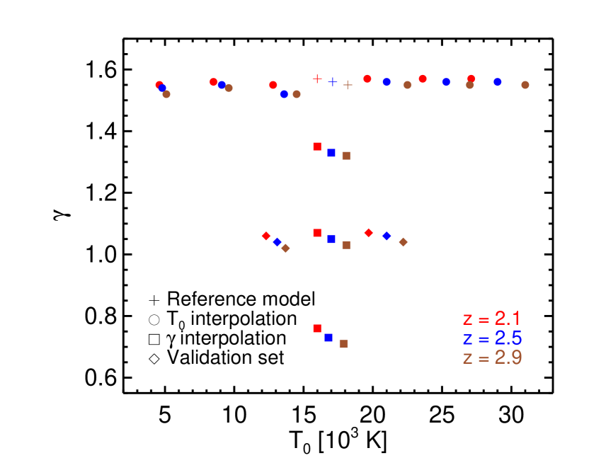
Figure 5: Simulations used in our interpolation scheme: reference model (crosses), $T_{0}$ interpolation (circles), $\gamma$ interpolation (squares) and the validation set (diamonds). Further information about the simulations may be found in Table 3.

Figure 6: Comparison of the wavelet PDF calculated with our interpolation scheme (dotted) to the PDF from a direct simulation (solid), for two validation simulations, C10 (upper) and E10 (lower). The agreement is satisfactorily within the uncertainties that we have assumed.

4.2 Parameter sampling

In order to estimate the astrophysical and cosmological parameters and their uncertainties, we use a sampling-based approach. Bayes’ theorem can be written as ${\cal L}(\mathbf{D}|\theta)\pi(\theta)=ZP(\theta)$, where ${\cal L}$ is the likelihood of the data $\mathbf{D}$ given parameters $\theta$, $\pi(\theta)$ are priors on the parameters, $Z=\int d\theta\pi(\theta){\cal L}$ is the model likelihood or ‘evidence’ and $P(\theta)$ is the sought-after posterior distribution of the parameters.

We perform posterior sampling using the ‘nested sampling’ algorithm, which is technique proposed by Skilling (2004), principally for estimation of the evidence $Z$ with posterior sampling as a by-product. We have chosen this algorithm because it is well-suited for sampling likelihoods that are multi-modal, strongly degenerate, or non-Gaussian. To briefly summarise the nested sampling method, the multi-dimensional integral $Z$ is remapped onto a particular one dimensional integral. A key ingredient for this kind of sampling is then the ability to draw uniform random samples from the remaining region of parameter space delimited by an iso-likelihood surface. We made use of the publicly available implementation MultiNest (Feroz & Hobson, 2008; Feroz et al., 2009), in which those regions bounded by iso-likelihood contours are approximated by ellipsoids (Mukherjee et al., 2006). We run MultiNest in a configuration with 500-1000 ‘live points’ and with a relatively low sampling efficiency of around $10^{-3}$. The posterior samples are then analysed with the getdist package (Lewis & Bridle, 2002) in order to extract two-dimensional and one-dimensional marginalised constraints.

4.3 IGM parametrization and priors

The next step in our analysis is to parametrize the redshift evolution of the quantities we wish to constrain. We therefore investigate a model for the possible redshift dependence of the IGM parameters in which $T_{0}$, $\gamma$ and $\tau_{\rm eff}$ are allowed to vary as piecewise constants centred on the redshifts $z=[2.1,2.5,2.9]$, and which will be referred to as the ‘redshift bins parametrization’.

We have put wide flat priors on the IGM parameter ranges, $5<T_{0}/{\rm 10^{3}K}<50$, $0.5<\gamma<1.7$, $0.075<\tau_{\rm eff}[z=2.1]<0.2$, $0.13<\tau_{\rm eff}[z=2.5]<0.3$, and $0.2<\tau_{\rm eff}[z=2.9]<0.5$; here the $\tau_{\rm eff}$ prior approximates and encompasses the ranges allowed from Figure 13 of Kim et al. (2007). For the cosmological parameters, we have imposed the flat priors $0.6<\sigma_{8}<1.0$, $0.9<n_{s}<1$ and $0.20<\Omega_{\rm m}<0.32$, and $60<H_{0}<84$ which is intended to be a conservative range encompassing the region favoured by WMAP (Larson et al., 2011) and $H_{0}$ constraints (Freedman et al., 2001).

Note that more restrictive power-law parametrizations for $T_{0}(z)$, $\gamma(z)$ and $\tau_{\rm eff}(z)$ have been investigated by a number of authors (Viel et al., 2009; Bird et al., 2011). Owing to the potentially complex and uncertain phenomenology suggested by theoretical models of the IGM, we have opted for the more general redshift bins parametrization.

4.4 The effect of astrophysical and cosmological parameters on the wavelet PDF

Having described our IGM parametrization and implemented our interpolation scheme, we are now in a position to demonstrate how the wavelet amplitude PDF depends on the astrophysical parameters, $T_{0}$, $\gamma$ and $\tau_{\rm eff}$, before proceeding to present our temperature constraints. This is illustrated in Figure 7, from which we may confirm the phenomenology for the wavelet amplitude PDF found in Lidz et al. (2010): the wavelet amplitude PDF shifts to smaller values for higher temperatures owing to Doppler broadening and Jeans smoothing which suppresses small scale power. Higher values of $\gamma$ also shift the peak of the wavelet PDF to lower amplitudes at fixed $T_{0}$ due to the decreased thermal smoothing associated with absorption from overdense gas, which dominates the Lyman-$\alpha$ absorption at $z<3$ (e.g. Becker et al. 2011). Increasing $\tau_{\rm eff}$ lowers the characteristic gas density probed by the Lyman-$\alpha$ absorption, shifting the peak amplitude of the wavelet PDF to higher values due to the colder underdense gas present for our fiducial $\gamma=1.6$. Clearly the uncertainty in $\tau_{\rm eff}$ needs to be marginalised over in order to estimate $T_{0}$ and $\gamma$, as any physical effect that affects the power spectrum of the Lyman-$\alpha$ absorption lines at small scales $k>0.1$ s/km will also substantially affect the wavelet amplitude PDF.

Finally, the effect of the cosmological parameters on the wavelet amplitude is found to be weak, except for $\sigma_{8}$ that has an slight impact on the wavelet PDF at redshift $z=2.1$ as we demonstrate in Figure 12 of Appendix A.1. The effect appears not to be as simple as a shift in the wavelet amplitude PDF as might be expected for a change in the power spectrum, as argued by Lidz et al. (2010). Our explicit simulations of the effect of varying $\sigma_{8}$ show a change in the width of the wavelet PDF in the lower redshift bin, where structure formation is more advanced.

Figure 7: The predicted wavelet amplitude PDF at redshifts $z=[2.1,\,2.5,\,2.9]$ (left to right columns) for our fiducial cosmological parameters. Top panels: varying $T_{0}$. The wavelet PDF shifts to lower values for higher temperatures owing to the suppression of power at small scales. Middle panels: varying $\gamma$. Here $\gamma$ defines the slope of the temperature-density relation, and a higher value for $\gamma$ leads to a higher value for the temperature at fixed $T_{0}$ in the overdense gas predominantly probed by the Lyman-$\alpha$ forest at $z<3$. Bottom panels: varying $\tau_{\rm eff}$. Increasing $\tau_{\rm eff}$ decreases the mean transmitted flux and shifts the characteristic density probed by the Lyman-$\alpha$ forest to lower values. These regions are cooler for our fiducial $\gamma=1.6$ than more overdense regions, leading to shift towards higher values of the wavelet amplitude.

5 Results

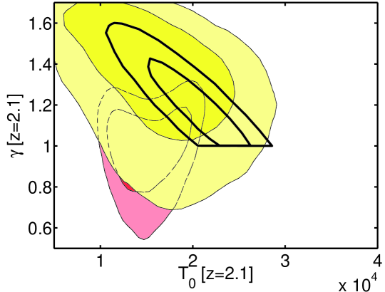
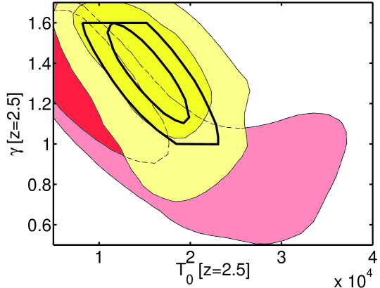
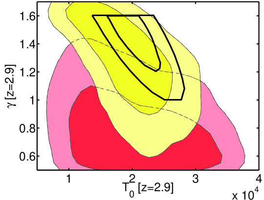
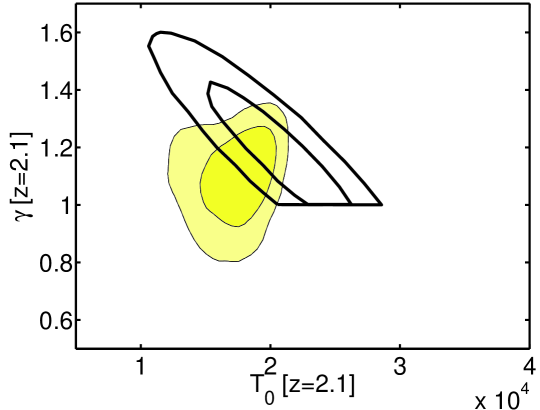
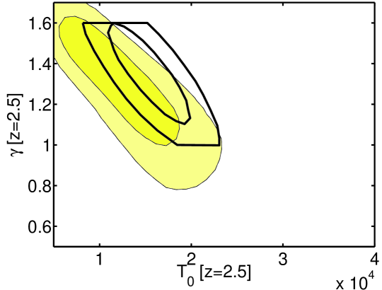
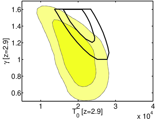
Figure 8: Upper panels: constraints on the IGM thermal parameters $T$ and $\gamma$ from our implementation of wavelet PDF analysis (yellow, light filled contours), compared with our reanalysis of the flux PDF from Viel et al. (2009) (red, dark filled contours) and the 1$\sigma$ and 2$\sigma$ constraints from Lidz et al. (2010) which assume a prior $\gamma=1.0-1.6$ (black contours). Lower panels: the joint constraints from the wavelet and flux PDF (filled contours) again compared to the Lidz et al. (2010) wavelet PDF constraints.

We now turn to describing the results of our analysis. Briefly, to restate the main aim of this work, we wish to compare the IGM cosmological and astrophysical constraints derived from our reanalysis of the Lyman-$\alpha$ flux PDF of Kim et al. (2007) with our new constraints derived from the wavelet amplitude PDF. We apply these two methodologies to the same dataset for the first time, enabling us to explore any systematic differences between these approaches. The computation of the flux PDF likelihood is performed in a similar way to Viel et al. (2009), using a second-order Taylor expansion of the cosmological and astrophysical parameter space. We have extended the Viel et al. (2009) analysis of the Kim et al. (2007) PDF to use our redshift bins parametrization, thereby dividing the data set into three redshift bins as opposed to using a single power-law parametrization as in Viel et al. (2009). Following Viel et al. (2009), we also fit the simulations to the observed flux PDF in the flux range $F=0.1$–$0.8$ only, in order to minimise the effect of continuum uncertainties on our results.

5.1 Constraints on the IGM thermal history

Our main results are shown in Figure 8, which displays the 1$\sigma$ and 2$\sigma$ contours obtained from our analysis of the wavelet PDF (yellow contours) and the flux PDF (red contours). Firstly, we note that the values of $T_{0}$ and $\gamma$ inferred from our analysis of the wavelet and flux PDF are in broad agreement with each other, and are formally consistent within 1$\sigma$. In part this is because in this analysis we have, in the first instance, left $\tau_{\rm eff}$ as free parameter, which enlarges the parameter space consistent with the wavelet PDF due to the degeneracy between $\tau_{\rm eff}$ and $T_{0}$. It is also apparent, however, that the flux PDF constraints generally favour a lower value for the temperature-density relation slope, $\gamma$, compared to the wavelet PDF (e.g. Bolton et al. 2008; Viel et al. 2009). This implies there may be a systematic difference between the two methodologies.

Motivated by recent suggestions about possible systematics in the flux PDF due to continuum placement (Lee, 2011; McQuinn et al., 2011) we have investigated whether the wavelet and flux PDF show any sensitivity to the continuum level assumed. We performed a check by lowering the continuum level on the synthetic spectra by 3 per cent (e.g. Tytler et al. 2004; Faucher-Giguère et al. 2008), and then recalculating both the flux and wavelet PDF for our $z=2.98$ simulations, for two models with $T_{0}[10^{3}$K$]=18$, $\tau_{\rm eff}=0.350$ and $\gamma=1.6$ and $0.7$ respectively. Figures showing the results from these tests are shown in Figure 14 in the appendix. We conclude that while the flux PDF shows some sensitivity to the continuum level at high ($F>0.8$) and low ($F<0.1$) fluxes (data that have not been used in our fit), the overall change in the fit is small compared to the improvement in the fit from moving (for example) from $\gamma=1.6$ to $\gamma=0.7$. It therefore appears that continuum errors do not fully explain the tendency for the flux PDF to favour somewhat lower values of $\gamma$ at $z=3$.

For comparison, we also show in Figure 8 results from the wavelet PDF analysis of Lidz et al. (2010) extracted from their Figure 25. The three Lidz et al. (2010) redshift bins are $z=[2.1,\,2.6,\,3.0]$ which roughly correspond to our own redshift bins. Note that Lidz et al. (2010) imposed a prior $\gamma=1.0-1.6$ and regarded their constraints as approximate, cautioning against taking their results too literally. Therefore, in interpreting their results we will attempt to make an allowance for the caveat they expressed by examining their 2$\sigma$ constraints. Lidz et al. (2010) have analysed just over double the number of spectra used in this study by using the 40 spectra reduced by Dall’Aglio et al. (2008); sixteen of our eighteen spectra also appear in their sample. Our wavelet PDF error bar treatment is probably the more conservative, explaining why our constraints are somewhat looser. In general, however, we find very good agreement with the Lidz et al. (2010) constraints, which is encouraging given the independently reduced observational data set and different simulation method used by these authors.

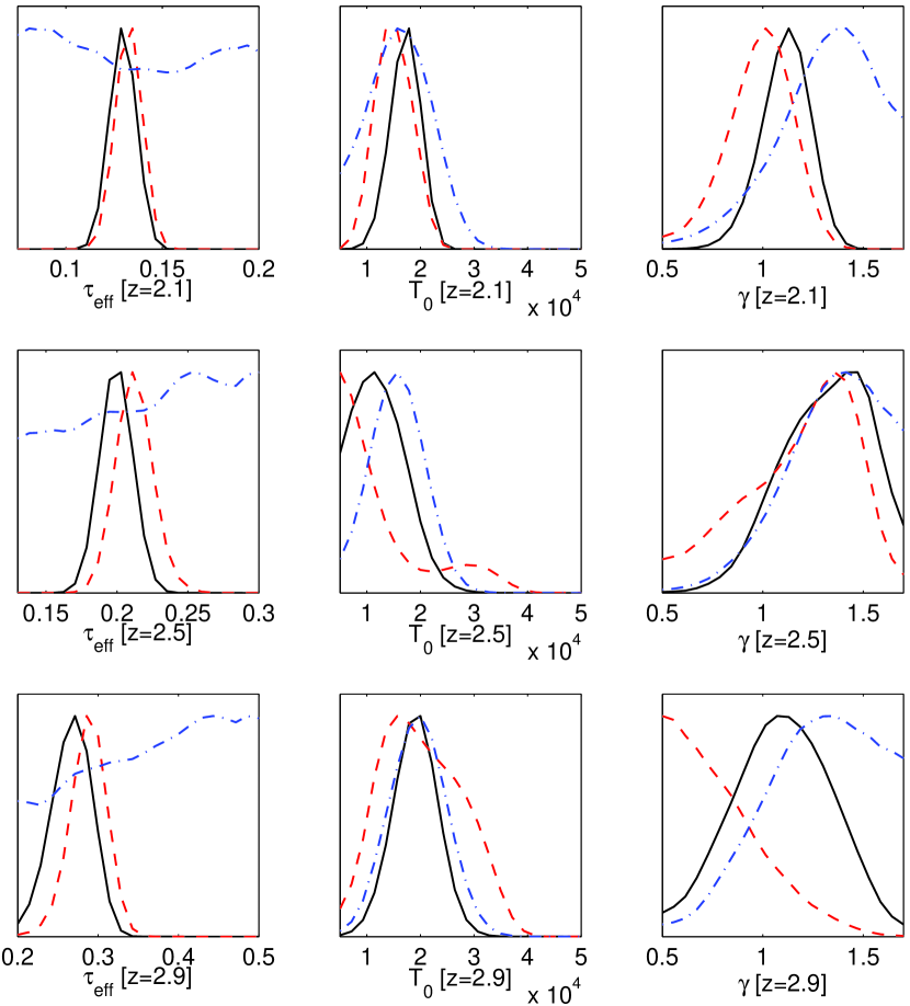
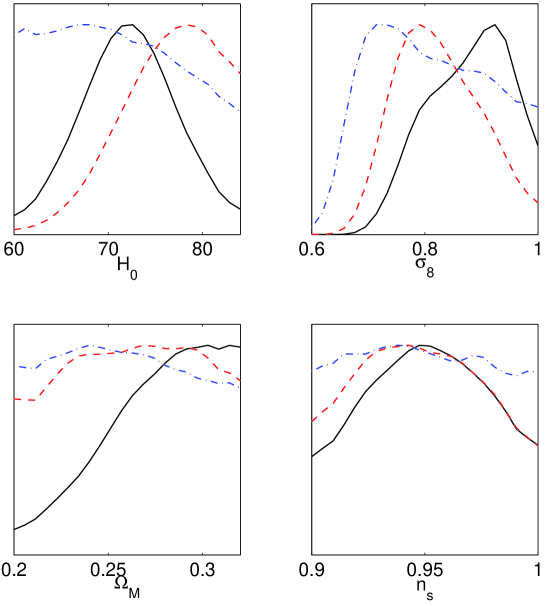
Figure 9: One dimensional marginalised constraints, corresponding to the two dimensional constraints shown in Figure 8. Note the constraints are shown as relative probabilities in each panel. The IGM temperature inferred from the wavelet amplitude PDF (dot dashed, blue) is in broad agreement with the flux PDF value (dashed red). The cosmological parameters are unconstrained, as is $\tau_{\rm eff}$ for the wavelet amplitude PDF. The joint constraints are also shown (solid, black).

Our one dimensional parameter constraints are shown in Figure 9 in which we can compare the results from the wavelet and flux PDF side by side. It is clear that the cosmological parameters are unconstrained by the wavelet PDF owing to their weak effect, with perhaps only a lower bound on $\sigma_{8}$ being found. The flux PDF – a one point statistic of the unfiltered spectra – puts the stronger constraint on the values of $\tau_{\rm eff}$; the values of $\tau_{\rm eff}$ we find for these redshift bins agree at the 1-2$\sigma$ level with those determined by Faucher-Giguère et al. (2008). This is in fact our main motivation for performing a ‘joint analysis’ of the flux PDF and wavelet PDF together (combining their likelihoods with equal weight), in order to self-consistently add the $\tau_{\rm eff}$ constraint derived from the flux PDF onto the parameter space consistent with the observed wavelet PDF. The final results for the joint analysis are summarised in Table 2 and the lower three panels of Figure 8. The joint constraints favour an IGM temperature-density relation which is close to isothermal, with temperatures at mean density which lie in the range $10\,000$–$20\,000\rm\,K$. However, the 1$\sigma$ uncertainties are too large to infer any significant redshift evolution in these quantities.

5.2 Comparison with previous constraints

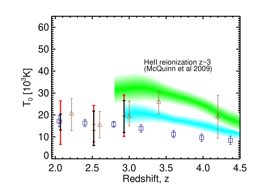
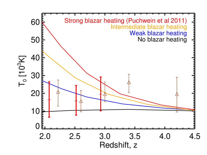
Figure 10: A comparison of our constraints with literature models for $T(z)$. Our constraints are the thick data points: Wavelet PDF $2\sigma$ (outer, red), joint analysis $2\sigma$ (inner, black), Lidz et al. (2010) wavelet analysis $2\sigma$ (triangles), and the Becker et al. (2011) curvature analysis $2\sigma$ (squares) which assumes $\gamma=1.3$. The shaded regions (upper panel) are two He$\,\rm\scriptstyle II\$reionisation models from McQuinn et al. (2009) (‘S4b’ upper, ‘D1’ lower with quasar UV spectral indices of $0.6$ and $1.6$, respectively) while the lines (lower panel) show the temperature at mean density of the blazar heating models from Puchwein et al. (2011).

Finally, we compare our results to previous constraints in the literature and consider the implications for the thermal history of the IGM. In Figure 10 we present a comparison of our results to models for the redshift evolution of the temperature at mean density, $T_{0}(z)$, from the literature. We show our joint constraints on $T_{0}$ (black error bars) and from the wavelet PDF alone (red error bars) together with the models of He$\,\rm\scriptstyle II\$reionisation from McQuinn et al. (2009) (upper panel) and blazar heating from Puchwein et al. (2011) (lower panel). Specifically, we have compared the available data with the ‘D1’ and ‘S4b’ models from McQuinn et al. (2009); the latter model implements a harder quasar UV spectral index of $0.6$ compared to their fiducial $1.6$. Our constraints are generally consistent with the McQuinn et al. (2009) model of He$\,\rm\scriptstyle II\$reionisation, with the softer UV spectral index model preferred.

The wavelet only constraints tend to favour the weak blazar heating model of Puchwein et al. (2011), whose median temperature at mean density is shown. In contrast, Puchwein et al. (2011) concluded that their intermediate blazar heating was preferred based on a comparison of the temperature of their models calculated at the ‘optimal overdensity’ (which rises to $\Delta\sim 6$ at $z=2$) probed by the Becker et al. (2011) curvature constraints. The differences between the blazar heating models are more pronounced at mean density; the temperature-density relations predicted by Puchwein et al. (2011) are similar for all models at $\Delta\geq 2$–$3$, which partially accounts for why Puchwein et al. (2011) conclude the intermediate model is favoured. We note, however, the wavelet PDF is sensitive to gas temperatures over a range of densities (including the mean density) as it is a distribution rather than a single number (i.e. the curvature statistic used by Becker et al. 2011). A precise measurement of the temperature-density relation could in principle rule out the blazar heating model if $\gamma>1$, as the volumetric heating rate used in the blazar heating models produce a strongly inverted temperature-density relation by $z=2$.

We also compare our constraints on $T_{0}$ with the measurements of Lidz et al. (2010), also using the wavelet PDF technique, and the curvature measurements of Becker et al. (2011) (plotted assuming $\gamma=1.3$, which is within $\sim 1.5\sigma$ of our joint constraints in all redshift bins). Note that although they used a different measurement technique and data, Becker et al. (2011) use the same set of hydrodynamical simulations as us. There is good agreement between the measurements at $z<3$, although there does appear to be some tension between the Becker et al. (2011) and Lidz et al. (2010) results in the redshift range $z=3-3.5$. As pointed out by Becker et al. (2011), however, differences in the effective optical depth assumed in the two studies may play a role here; as we have demonstrated the wavelet PDF is rather sensitive to $\tau_{\rm eff}$. The Becker et al. (2011) constraints also have significantly smaller error bars compared to the wavelet PDF measurements. Note, however, the Becker et al. (2011) measurements do not attempt to simultaneously measure both $T_{0}$ and $\gamma$. As noted previously, they instead measure the IGM temperature at the characteristic density, $\bar{\Delta}(z)$, probed by the Lyman-$\alpha$ forest. Their constraints do not marginalise over the uncertain values of $\gamma$ and $\tau_{\rm eff}$, and so a direct comparison of their uncertainties to our results is less straightforward.

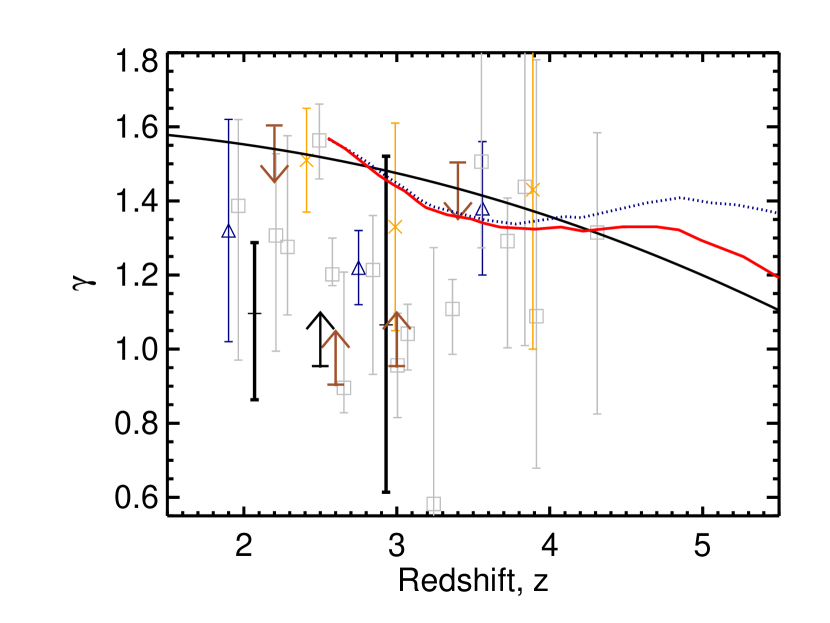
Figure 11: A comparison of our constraints on the slope of the temperature-density relation with various models for $\gamma(z)$ and other observational constraints from the literature. Our $2\sigma$ constraints and limit from the joint analysis (thick, black error bars and arrow), can be compared with the 2$\sigma$ limits from Lidz et al. (2010) (brown arrows), the 1$\sigma$ constraints from Ricotti et al. (2000) (triangles, navy), the 1$\sigma$ constraints from Schaye et al. (2000) (squares, grey) and the 1$\sigma$ constraints from McDonald et al. (2001) (crosses, orange). The extended solid line shows a model with sudden He$\,\rm\scriptstyle II\$reionisation heating the IGM to $25\,000$ K at $z=6$ (solid), while the broken lines are the ‘L1’ and ‘L1b’ models of He$\,\rm\scriptstyle II\$reionisation (solid and dotted) from McQuinn et al. (2009), which implement $\gamma=1.3$ and 1.0 at $z=6$, respectively.

In Figure 11 we attempt an analogous comparison of our constraints (thick black error bars) with the available models for $\gamma(z)$ as well as previous measurements. Our results are shown with the analytical reionisation models of Hui & Gnedin (1997) (with $T_{\rm reion}=25\,000$ K at $z=6$) and the extended He$\,\rm\scriptstyle II\$reionisation models ‘L1’ and ‘L1b’ from the radiative transfer simulations of McQuinn et al. (2009), which implement $\gamma=1.3$ and 1.0 at $z=6$, respectively. We compare our results with the limits from Lidz et al. (2010), and measurements from Ricotti et al. (2000), Schaye et al. (2000) and McDonald et al. (2001). Overall, it is clear that $\gamma$ remains relatively poorly constrained, although the data appear to prefer a temperature-density relation which is shallower than the $\gamma\sim 1.6$ expected if He$\,\rm\scriptstyle II\$reionisation occurred at $z\gg 3$. Overall, we find our results are in agreement with previous studies of the IGM temperature that suggest there may be additional heating in the IGM at $z<4$, most likely due to the reionisation of He$\,\rm\scriptstyle II\$by quasars (see also recent studies of the He$\,\rm\scriptstyle II\$Lyman-$\alpha$ forest, e.g. Shull et al. 2010; Worseck et al. 2011; Syphers et al. 2011). We conclude improved measurements of the slope of the temperature-density relation will be required for testing blazar heating models in detail.

		Wavelet PDF	Flux PDF	Joint analysis
$\left<z\right>=2.1$	$T_{0}\,[10^{3}\,{\rm K}]$	$16\pm 5$	$15\pm 3$	$17\pm 2$
	$\gamma$	$>0.86$	$0.99\pm 0.14$	$1.11\pm 0.11$
	$\tau_{\rm eff}$	$(0.14\pm 0.04)$	$0.133\pm 0.004$	$0.130\pm 0.004$
$\left<z\right>=2.5$	$T_{0}\,[10^{3}\,{\rm K}]$	$16\pm 4$	$14\pm 9$	$13\pm 4$
	$\gamma$	$>0.92$	$>0.69$	$>0.95$
	$\tau_{\rm eff}$	$(0.22\pm 0.05)$	$0.212\pm 0.011$	$0.200\pm 0.009$
$\left<z\right>=2.9$	$T_{0}\,[10^{3}\,{\rm K}]$	$20\pm 5$	$21\pm 7$	$19\pm 4$
	$\gamma$	$>0.80$	$<1.24$	$1.1\pm 0.2$
	$\tau_{\rm eff}$	$(0.36\pm 0.09)$	$0.290\pm 0.019$	$0.27\pm 0.02$

Table 2: 1$\sigma$ constraints on the IGM thermal parameters for the wavelet PDF, flux PDF and joint analysis. We find broad consistency between the methods, with the flux PDF favouring a slightly lower value of $\gamma$. Entries in parentheses are prior dominated (no detection) and the limits quoted are 95% confidence.

6 Conclusions

We have analyzed eighteen metal cleaned Lyman-$\alpha$ forest spectra in the redshift range 1.7–3.2 using both the flux PDF and wavelet PDF. The results have been interpreted using a suite of hydrodynamical simulations to place constraints on the thermal state of the intergalactic medium while marginalizing over the uncertainty in the cosmological parameters. Our wavelet analysis is similar to the analysis performed Theuns et al. (2002), following most closely the technique employed by Lidz et al. (2010), but using independently reduced spectra and a different approach to simulating the IGM. An analysis of the constraints on the IGM thermal state obtained from the flux PDF using the same data set furthermore enables us to explore any systematic differences between the two methodologies. The main results of our study are as follows:

• The constraints on the IGM thermal state at $z=1.7$–$3.2$ derived from the wavelet PDF and flux PDF analysis are formally consistent with each other within the rather large uncertainties. However, we find there is some mild tension between the two measurements, with the flux PDF measurements generally preferring a lower value for the slope of the temperature-density relation at all redshifts.
  

• We have checked that the impact of a continuum which has been placed 3 per cent too low on the wavelet and flux PDF is small compared to the effect of varying other free parameters such as $T_{0}$, $\gamma$ and $\tau_{\rm eff}$. The flux PDF is indeed more sensitive to changes in the continuum placement, but the effect remains small and is minimal within the flux range of $F=[0.1,0.8]$ we fit in our analysis. We conclude it is unlikely that the continuum placement is fully responsible for the systematic offset found in the wavelet and flux PDF constraints.
  

• We have explicitly confirmed that varying cosmological parameters within a narrow range has little impact on the wavelet amplitude PDF, with the strongest effect being that of $\sigma_{8}$ in our lowest redshift bin. We also confirm that there is a significant degeneracy between the parameters $T_{0}$, $\gamma$ and $\tau_{\rm eff}$ inferred from the wavelet amplitude PDF.
  

• The flux PDF puts a much stronger constraint on $\tau_{\rm eff}$ compared to the wavelet PDF. We therefore perform a joint analysis of the flux PDF and wavelet PDF in order to add the $\tau_{\rm eff}$ constraint derived from the flux PDF. We find the joint constraints on the IGM temperature at mean density, $T_{0}$, obtained at $z=[2.1,2.5,2.9]$ are in good agreement with other recent measurements. The constraints are consistent with the models of McQuinn et al. (2009), in which an extended He$\,\rm\scriptstyle II\$reionisation epoch completes around $z=3$, driven by quasars with an EUV index of $\alpha\simeq 1.6$. We have also performed a rudimentary comparison with the recently proposed blazar heating models of Puchwein et al. (2011), and find their weak blazar heating matches our $T_{0}$ constraints most closely.
  

• We find the slope of the temperature-density relation obtained from the joint analysis is consistent with $\gamma\sim 1.1$–$1.3$, although the uncertainties on this measurement remain large and remain consistent with an inverted ($\gamma<1$) temperature-density relation within $1$–$1.5\sigma$. A more precise measurement of the temperature-density relation will be necessary for stringently testing competing IGM heating models, such as the volumetric heating rate from blazar heating which produces a strongly inverted temperature-density relation by $z=2$ (Chang et al. 2011).

Overall, our results are consistent with previous observations that indicate there may be additional sources of heating in the IGM at $z<4$. This heating could be due to a number of effects such as an extended epoch of He$\,\rm\scriptstyle II\$reionisation which has yet to complete at $z=3$ (Shull et al., 2010; Worseck et al., 2011; Syphers et al., 2011), heating of the low density IGM by blazars (Puchwein et al., 2011) or feedback either in the form of galactic winds and/or AGN feedback (Tornatore et al., 2010; Booth & Schaye, 2012). We note, however, the latter will provide only a partial explanation due to the small volume filling factor of the shock-heated gas (Theuns et al. 2002).

We believe that analyses of the flux PDF (Viel et al. 2009; Calura et al. 2012), the wavelet PDF (Lidz et al. 2010) and other techniques such as the curvature (Becker et al. 2011) and absorption line widths (Schaye et al. 2000) provide generally consistent constraints on the IGM thermal state at $z<3$ when applied to high resolution spectra. This is encouraging given the wide range of different methodologies used in the existing literature. However, significant uncertainties on measurements of the IGM thermal state remain. Ideally, one should also aim at reaching full consistency between different data sets (high and low resolution QSO spectra) as well as different methods (see e.g. Viel et al. 2009). In the near future, large scale surveys of the Lyman-$\alpha$ forest at moderate spectral resolution, such as the SDSS Baryon Oscillation Spectroscopic Survey (BOSS) (Slosar et al. 2011), will provide valuable new insights into the physical state of the IGM with a high degree of statistical precision. Fully understanding the potential systematic uncertainties associated with these measurements are therefore vital for further unravelling the thermal history of the IGM following reionisation.

Appendix A Additional material

A.1 Dependence of the wavelet amplitude PDF on cosmological parameters

In this appendix we explicitly show the wavelet amplitude PDF depends almost negligibly on the cosmological parameters in our analysis. Figure 12 shows the effect of varying $H_{0}$, $\sigma_{8}$, $\Omega_{\rm m}$, and $n_{\rm s}$ on the wavelet PDF.

Figure 12: The wavelet amplitude PDF obtained from simulated spectra varying a single cosmological parameter about the fiducial model. Top left: Varying $H_{0}$. Top right: Varying $\sigma_{8}$. Bottom left: Varying $\Omega_{\rm m}$. Bottom right: Varying $n_{\rm s}$. The wavelet amplitude PDF has a very weak dependence on the cosmological parameters, but with a mild dependence on $\sigma_{8}$ in our lowest redshift bin $z=2.1$.

A.2 Simulation parameters and convergence tests

In Table 3 we list the parameters of our simulations, and catalogue how they have been used in the interpolation scheme described in Section 4.1. Using simulations R1, R2, R3 and C15 we have tested the convergence of the wavelet amplitude PDF with gas particle mass and box size. Figure 13 demonstrates the stability of the wavelet amplitude PDF under this change.

Table 3: Parameters of the simulations used for describing the thermal state of the IGM: $L$ is the comoving box-length; $N$ the number of gas and dark matter particles in the simulation; $M_{\rm gas}$ is the mass of each gas particle in the simulation box; $\zeta$ and $\xi$ are the scaling parameters used to modify the photo-heating rates. $T_{0}$ and $\gamma$ are not a priori parameters of the simulations, but are determined by fitting the temperature-density relation at each redshift. The table is divided into five sections: our reference model (D15); simulations for interpolating over $\gamma$; simulations for interpolating over $T_{0}$; the validation set; resolution and box-size checks.

Model	$L$	$N$	$M_{\rm gas}$	$\zeta$	$\xi$	$T_{0}/10^{3}{\rm K}$	$T_{0}/10^{3}{\rm K}$	$T_{0}/10^{3}{\rm K}$	$\gamma$	$\gamma$	$\gamma$
	$[h^{-1}$ Mpc$]$		$[10^{4}h^{-1}M_{\varodot}]$			$[z=2.17]$	$[z=2.55]$	$[z=2.98]$	$[z=2.17]$	$[z=2.55]$	$[z=2.98]$
D15	10	$2\times 512^{3}$	$9.2$	2.20	0.00	16.0	17.1	18.2	1.57	1.56	1.55
D07	10	$2\times 512^{3}$	$9.2$	2.20	-1.60	16.0	16.8	17.9	0.76	0.73	0.71
D10	10	$2\times 512^{3}$	$9.2$	2.20	-1.00	16.0	17.0	18.1	1.07	1.05	1.03
D13	10	$2\times 512^{3}$	$9.2$	2.20	-0.45	16.0	17.0	18.1	1.35	1.33	1.32
A15	10	$2\times 512^{3}$	$9.2$	0.3	0.00	4.6	4.8	5.1	1.55	1.54	1.52
B15	10	$2\times 512^{3}$	$9.2$	0.8	0.00	8.5	9.1	9.6	1.56	1.55	1.54
C15	10	$2\times 512^{3}$	$9.2$	1.45	0.00	12.4	13.2	14.0	1.57	1.56	1.54
E15	10	$2\times 512^{3}$	$9.2$	3.10	0.00	19.6	21.0	22.5	1.57	1.56	1.55
F15	10	$2\times 512^{3}$	$9.2$	4.20	0.00	23.6	25.3	27.0	1.57	1.56	1.55
G15	10	$2\times 512^{3}$	$9.2$	5.30	0.00	27.1	29.0	31.0	1.57	1.56	1.55
C10	10	$2\times 512^{3}$	$9.2$	1.45	-1.00	12.3	13.1	13.7	1.06	1.04	1.02
E10	10	$2\times 512^{3}$	$9.2$	3.10	-1.00	19.7	21.0	22.2	1.07	1.06	1.04
R1	10	$2\times 256^{3}$	$7.4$	1.45	0.00	12.5	13.2	14.0	1.56	1.54	1.53
R2	10	$2\times 128^{3}$	$5.9$	1.45	0.00	12.8	13.5	14.3	1.54	1.53	1.51
R3	20	$2\times 256^{3}$	$5.9$	1.45	0.00	12.8	13.6	14.3	1.54	1.53	1.51
R4	40	$2\times 512^{3}$	$5.9$	1.45	0.00	12.8	13.6	14.5	1.55	1.52	1.52

Figure 13: Convergence of the wavelet amplitude PDF with increasing gas particle mass at fixed box size (upper row) and increasing box size at fixed gas particle mass (lower row). Our conclusions from these tests are described in Section 2.2.

A.3 Continuum test

Figure 14 demonstrates the effect of lowering the continuum on the simulated spectra by 3 per cent on the wavelet amplitude and flux PDFs. A brief discussion of the results from this test is provided in Section 5.1.

Figure 14: The effect of the continuum level on the wavelet amplitude and flux PDFs at redshift $z=2.9$. In the left panels we show the wavelet PDFs for the simulations D15 (above) and D07 (below); in the right panels we show the flux PDFs for the same simulations. The dotted lines are the results for the native continuum level in the simulations (indicated with regular) whereas the dashed lines are for a continuum level which has been lowered by $3$ per cent. For comparison, we also show with a solid line the data with the error bars used in the two analyses.

References

- Becker et al. (2011) Becker G. D., Bolton J. S., Haehnelt M. G., Sargent W. L. W., 2011, MNRAS, 410, 1096
- Becker et al. (2007) Becker G. D., Rauch M., Sargent W. L. W., 2007, ApJ, 662, 72
- Becker et al. (2001) Becker R. H., Fan X., White R. L., et al. 2001, AJ, 122, 2850
- Bird et al. (2011) Bird S., Peiris H. V., Viel M., Verde L., 2011, MNRAS, 413, 1717
- Bolton et al. (2010) Bolton J. S., Becker G. D., Wyithe J. S. B., Haehnelt M. G., Sargent W. L. W., 2010, MNRAS, 406, 612
- Bolton et al. (2009) Bolton J. S., Oh S. P., Furlanetto S. R., 2009, MNRAS, 395, 736
- Bolton et al. (2008) Bolton J. S., Viel M., Kim T., Haehnelt M. G., Carswell R. F., 2008, MNRAS, 386, 1131
- Booth & Schaye (2012) Booth C. M., Schaye J., 2012, ArXiv e-prints
- Calura et al. (2012) Calura F., Tescari E., D’Odorico V., Viel M., Cristiani S., Kim T.-S., Bolton J. S., 2012, MNRAS submitted, arXiv:1201.5121
- Chang et al. (2011) Chang P., Broderick A. E., Pfrommer C., 2011, ApJ submitted, arXiv1106.5504
- Dall’Aglio et al. (2008) Dall’Aglio A., Wisotzki L., Worseck G., 2008, A&A, 491, 465
- Eisenstein & Hu (1999) Eisenstein D. J., Hu W., 1999, ApJ, 511, 5
- Fan et al. (2006) Fan X., Strauss M. A., Becker R. H., White R. L., et al. 2006, AJ, 132, 117
- Faucher-Giguère et al. (2008) Faucher-Giguère C.-A., Prochaska J. X., Lidz A., Hernquist L., Zaldarriaga M., 2008, ApJ, 681, 831
- Fendt & Wandelt (2007) Fendt W. A., Wandelt B. D., 2007, ApJ, 654, 2
- Feroz & Hobson (2008) Feroz F., Hobson M. P., 2008, MNRAS, 384, 449
- Feroz et al. (2009) Feroz F., Hobson M. P., Bridges M., 2009, MNRAS, 398, 1601
- Freedman et al. (2001) Freedman W. L., Madore B. F., Gibson B. K., Ferrarese L., et al. 2001, ApJ, 553, 47
- Furlanetto & Oh (2008) Furlanetto S. R., Oh S. P., 2008, ApJ, 681, 1
- Haardt & Madau (2001) Haardt F., Madau P., 2001, in D. M. Neumann & J. T. V. Tran ed., Clusters of Galaxies and the High Redshift Universe Observed in X-rays Modelling the UV/X-ray cosmic background with CUBA
- Hui & Gnedin (1997) Hui L., Gnedin N. Y., 1997, MNRAS, 292, 27
- Hui & Haiman (2003) Hui L., Haiman Z., 2003, ApJ, 596, 9
- Kim et al. (2007) Kim T., Bolton J. S., Viel M., Haehnelt M. G., Carswell R. F., 2007, MNRAS, 382, 1657
- Larson et al. (2011) Larson D. andDunkley J., Hinshaw G., Komatsu E., Nolta M. R., et al. 2011, ApJS, 192, 16
- Lee (2011) Lee K.-G., 2011, ApJ submitted, arXiv:1103.2780
- Lewis & Bridle (2002) Lewis A., Bridle S., 2002, Phys. Rev. D, 66, 103511
- Lidz et al. (2010) Lidz A., Faucher-Giguère C., Dall’Aglio A., McQuinn M., Fechner C., Zaldarriaga M., Hernquist L., Dutta S., 2010, ApJ, 718, 199
- Lidz et al. (2006) Lidz A., Heitmann K., Hui L., Habib S., Rauch M., Sargent W. L. W., 2006, ApJ, 638, 27
- Madau et al. (1999) Madau P., Haardt F., Rees M. J., 1999, ApJ, 514, 648
- McDonald et al. (2001) McDonald P., Miralda-Escudé J., Rauch M., Sargent W. L. W., Barlow T. A., Cen R., 2001, ApJ, 562, 52
- McDonald et al. (2000) McDonald P., Miralda-Escudé J., Rauch M., Sargent W. L. W., Barlow T. A., Cen R., Ostriker J. P., 2000, ApJ, 543, 1
- McQuinn et al. (2011) McQuinn M., Hernquist L., Lidz A., Zaldarriaga M., 2011, MNRAS, 415, 977
- McQuinn et al. (2009) McQuinn M., Lidz A., Zaldarriaga M., Hernquist L., Hopkins P. F., Dutta S., Faucher-Giguère C., 2009, ApJ, 694, 842
- Meiksin (2000) Meiksin A., 2000, MNRAS, 314, 566
- Mukherjee et al. (2006) Mukherjee P., Parkinson D., Liddle A. R., 2006, ApJ, 638, L51
- Pawlik et al. (2009) Pawlik A. H., Schaye J., van Scherpenzeel E., 2009, MNRAS, 394, 1812
- Peeples et al. (2010a) Peeples M. S., Weinberg D. H., Davé R., Fardal M. A., Katz N., 2010a, MNRAS, 404, 1281
- Peeples et al. (2010b) Peeples M. S., Weinberg D. H., Davé R., Fardal M. A., Katz N., 2010b, MNRAS, 404, 1295
- Puchwein et al. (2011) Puchwein E., Pfrommer C., Springel V., Broderick A. E., Chang P., 2011, MNRAS submitted, arXiv:1107.3837
- Raskutti et al. (2012) Raskutti S., Bolton J. S., Wyithe J. S. B., Becker G. D., 2012, MNRAS in press, arXiv:1201.5138
- Ricotti et al. (2000) Ricotti M., Gnedin N. Y., Shull J. M., 2000, ApJ, 534, 41
- Schaye et al. (2000) Schaye J., Theuns T., Rauch M., Efstathiou G., Sargent W. L. W., 2000, MNRAS, 318, 817
- Shull et al. (2010) Shull J. M., France K., Danforth C. W., Smith B., Tumlinson J., 2010, ApJ, 722, 1312
- Skilling (2004) Skilling J., 2004, in R. Fischer, R. Preuss, & U. V. Toussaint ed., American Institute of Physics Conference Series Vol. 735 of American Institute of Physics Conference Series, Nested Sampling. pp 395–405
- Slosar et al. (2011) Slosar A., Font-Ribera A., Pieri M. M., Rich J., Le Goff J.-M., Aubourg É., et al. 2011, J. Cosmology Astropart. Phys, 9, 1
- Springel (2005) Springel V., 2005, MNRAS, 364, 1105
- Syphers et al. (2011) Syphers D., Anderson S. F., Zheng W., Meiksin A., Haggard D., Schneider D. P., York D. G., 2011, ApJ, 726, 111
- Tepper-García (2006) Tepper-García T., 2006, MNRAS, 369, 2025
- Theuns et al. (1998) Theuns T., Leonard A., Efstathiou G., Pearce F. R., Thomas P. A., 1998, MNRAS, 301, 478
- Theuns et al. (2002) Theuns T., Viel M., Kay S., Schaye J., Carswell R. F., Tzanavaris P., 2002, ApJ, 578, L5
- Theuns & Zaroubi (2000) Theuns T., Zaroubi S., 2000, MNRAS, 317, 989
- Theuns et al. (2002) Theuns T., Zaroubi S., Kim T., Tzanavaris P., Carswell R. F., 2002, MNRAS, 332, 367
- Tittley & Meiksin (2007) Tittley E. R., Meiksin A., 2007, MNRAS, 380, 1369
- Tornatore et al. (2010) Tornatore L., Borgani S., Viel M., Springel V., 2010, MNRAS, 402, 1911
- Tytler et al. (2004) Tytler D., Kirkman D., O’Meara J. M., Suzuki N., Orin A., Lubin D., Paschos P., Jena T., Lin W.-C., Norman M. L., Meiksin A., 2004, ApJ, 617, 1
- Viel et al. (2009) Viel M., Bolton J. S., Haehnelt M. G., 2009, MNRAS, 399, L39
- Viel et al. (2004) Viel M., Haehnelt M. G., Springel V., 2004, MNRAS, 354, 684
- Worseck et al. (2011) Worseck G., nd Prochaska J. X., McQuinn M., Dall’Aglio A., et al. 2011, ApJ, 733, L24
- Zaldarriaga (2002) Zaldarriaga M., 2002, ApJ, 564, 153
- Zaldarriaga et al. (2001) Zaldarriaga M., Hui L., Tegmark M., 2001, ApJ, 557, 519