SUNDMAN STABILITY OF NATURAL PLANET SATELLITES

Abstract

The stability of the motion of the planet satellites is considered in the model of the general three-body problem (Sun-planet-satellite). ”Sundman surfaces” are constructed, by means of which the concept ”Sundman stability” is formulated. The comparison of the Sundman stability with the results of Golubev’s $c^{2}h$ method and with the Hill’s classical stability in the restricted three-body problem is performed. The constructed Sundman stability regions in the plane of the parameters ”energy - moment of momentum” coincide with the analogous regions obtained by Golubev’s method, with the value $(c^{2}h)_{cr}$.

The construction of the Sundman surfaces in the three-dimensional space of the specially selected coordinates $xyR$ is carried out by means of the exact Sundman inequality in the general three-body problem. The determination of the singular points of surfaces, the regions of the possible motion and Sundman stability analysis are implemented. It is shown that the singular points of the Sundman surfaces in the coordinate space $xyR$ lie in different planes. Sundman stability of all known natural satellites of planets is investigated. It is shown that a number of the natural satellites, that are stable according to Hill and also some satellites that are stable according to Golubev’s method are unstable in the sense of Sundman stability.

PACS : 95.10.Ce

Key words: Hill stability: Sundman stability: planet satellites.

1 INTRODUCTION

The study of the motion stability of the planet satellites has been usually performed by means of the Hill surfaces (Hill, 1878) constructed either for the model of the restricted three-body problem (Proskurin, 1950), or for the problem of Hill (Hagihara, 1952). Since Golubev (1967, 1968, 1985) who developed the method it is sometimes referred to as $c^{2}h$ method for the general three-body problem, the stability analysis of the motions is usually carried out by Golubev’s method. This method is based on the famous Sundman inequality (Sundman, 1912).

The search for regions of stable motions in the general three-body problem is divided into two tasks:

- determination of stability regions in the plane of two free parameters — the constant of the energy integral and constant of the moment of momentum integral,

- determination of stable regions in the space of the coordinates used.

Actually Golubev (1967) carried out the complete solution of the first task by the introduction of ”the index of Hill stability” $s=c^{2}h$, where $h$ is the energy constant, and $c$ is the moment of momentum constant. Golubev showed that the curve $s=s_{cr}$ is the boundary of the stability region in the plane of $ch$, where the value of $s_{cr}$ is calculated at the Eulerian inner libration point $L_{2}$ with the use of the known equation of fifth power as some function of body masses.

The solution of the second problem is considerably more complex, since it requires the construction of the Sundman surfaces in the multidimensional space of the coordinates used. For the solution of this problem Golubev (1968) applied the simplified Sundman inequality, with the aid of which the solution of problem leads to the construction of Hill curves in the plane of two rectangular coordinates $x$ and $y$.

Some authors (Marchal, Saari, 1975), (Zare, 1976), (Marchal, Bozis, 1982), (Marchal, 1990) have elaborated the Golubev’s results with the use of the simplified Sundman inequality.

The construction of the regions of possible motions in the space of the selected coordinates with the use of the exact Sundman inequality is hindered by the large number of variables. Thus, in the relative or Jacobian coordinate systems the number of the variables is six: three coordinates of one body and three of the other. Therefore, the construction of the Sundman surfaces can be carried out in the six-dimensional space of these coordinates.

In the large series of works (Szebehely, Zare, 1977), (Walker, Emslie, Roy, 1980), (Donnison, Williams, 1983), (Donnison, 2009), (Li, Fu, Sun, 2010), (Donnison, 2010) and other authors the determination of the regions of the possible motions is carried out in the six-dimensional space of the Keplerian elements $a_{1},a_{2}$, $e_{1},e_{2}$, $i_{1}$ and $i_{2}$ or in the four-dimensional space $a_{1},a_{2}$, $e_{1}$ and $e_{2}$ for the planar problem.

At the same time, the construction of the Sundman surfaces and, thus, the determination of the regions of possible motions and stability regions can be conducted in the space of three variables. This substantially facilitates the readability of results and eases their application. This possibility is explained by the fact that the exact Sundman inequality depends on the coordinates only by means of three quantities — three mutual distances between the bodies.

The article (Lukyanov and Shirmin, 2007) is likely to be the first work that confirmed this possibility. In this work the mutual distances between the bodies are the rectangular coordinates. The existence of the Hill surfaces’s analogue for the general three-body problem in the space of the mutual distances is shown here using the exact Sundman inequality. The stability regions are determined in the space of the mutual distances and have the form of an infinite ”tripod”.

Lukyanov (2011) used another choice of three coordinates. The coordinate system is determined by the accompanying triangle of mutual positions of bodies. Namely, the origin of the coordinate system coincides with one of the bodies, the axis $x$ is directed towards the second body, the axis $y$ is perpendicular to the axis $x$ and lies in the plane of the triangle. In this coordinate system the position of all bodies is determined by three coordinates $x,y,R$, where $x$ and $y$ are the coordinates of the third body, and $R$ is the distance between the first and second bodies. The system of coordinates $xyR$ is to a certain degree similar to the rotating coordinate system in the restricted three-body problem following the motion of the basic bodies.

Then, in the space of the coordinates $xyR$ the Sundman surfaces are constructed, the singular points of surfaces (coinciding with the Euler and Lagrange libration points) are located, the regions of the possible motions and Sundman stability regions are determined. The stability region of any body relative to the other body in the space $xyR$ has the form, similar to an infinite ”spindle”. No restriction on the masses of bodies or their mutual positions is assumed in this case.

In the present work the method of constructing the regions of the possible motions (Sundman lobes) in the general three-body problem is presented. The Sundman stability analysis of the natural satellites of the planets is carried out, using the high-precision ephemeris of the natural satellites of planets calculated on the web-site ”Natural Satellite Data Center” (NSDC) (Sternberg Astronomical Institute, Moscow)

$(http://www.sai.msu.ru/neb/nss/index.htm)$.

2 SUNDMAN SURFACES

The regions of possible motions of bodies in the general three-body problem are determined by Sundman inequality

$$(U-C)J\geq B,$$ (1)

where the force function $U$ and the barycentric moment of inertia $J$ are determined by the expressions:

$$U=\frac{Gm_{1}m_{2}}{R_{12}}+\frac{Gm_{2}m_{3}}{R_{23}}+\frac{Gm_{3}m_{1}}{R_{31}},$$ (2)

$$J=\frac{m_{1}m_{2}R_{12}^{2}+m_{2}m_{3}R_{23}^{2}+m_{3}m_{1}R_{31}^{2}}{m},$$ (3)

$C=-h$ is the analogue of the Jacobi constant, $h$ is the energy constant, $B=c^{2}/2$ is the Sundman constant, $c$ is the constant of the integral of area.

Here: $G$ is the universal gravitational constant, $m_{1},m_{2},m_{3}$ are the masses of bodies, $m=m_{1}+m_{2}+m_{3}$ is the total mass of the system, $R_{12}$, $R_{23}$, $R_{31}$ are the mutual distances between the bodies.

Constants $C$ and $B$ are determined by the initial conditions in the barycentric coordinate system from the relationships:

$$\begin{array}[]{c}\displaystyle C=-h=U-m_{1}\frac{V_{1}^{2}}{2}-m_{2}\frac{V_{2}^{2}}{2}-m_{3}\frac{V_{3}^{2}}{2},\\ \displaystyle B=\frac{c^{2}}{2}=\frac{1}{2}(m_{1}\mathbf{r}_{1}\times\mathbf{V}_{1}+m_{2}\mathbf{r}_{2}\times\mathbf{V}_{2}+m_{3}\mathbf{r}_{3}\times\mathbf{V}_{3})^{2},\\ \end{array}$$ (4)

$\mathbf{r}_{i},\,\mathbf{V}_{i},\,(i=1,2,3)$ are the barycentric state and speed vectors of the bodies.

The boundary of the region of possible motions can be established if in (1) inequality is replaced with equality:

$$(U-C)J=B.$$ (5)

This equality determines the equation of the Sundman surface. In the general case the mutual distances in (5) depend on nine coordinates of three moving bodies, which substantially hampers the construction of the Sundman surfaces. The transformation to the relative coordinate system makes it possible to reduce the number of coordinates to six. However, in this case the construction of the Sundman surfaces should be conducted in the six-dimensional space. Furthermore, the number of coordinates can be reduced to three if the positions of bodies are determined by the following special coordinates.

The position of the body $M_{2}$ relative to the body $M_{1}$ will be characterized by the abscissa $R$ on the axis $M_{1}X$. we will define the position of the body $M_{3}$ relative to $M_{1}$ by the rectangular coordinates $X$ and $Y$ in the system of $M_{1}XY$, which always lies in the plane that passes through all three bodies. The positions of the bodies in the coordinate system $M_{1}XYR$ are defined by three quantities - coordinates $X$, $Y$ and $R$, which allows us to construct the Sundman surfaces in the three-dimensional space.

We will use a dimensionless system of coordinates $M_{1}xy$ making the substitution

$$X=Rx,\quad Y=Ry.$$ (6)

Then the mutual distances between the bodies can be expressed in terms of three quantities $x,y,R$. The Sundman surface equation transforms to the form of the functions of three variables

$$\begin{array}[]{c}\displaystyle S(x,y,R)=(U-C)J=\left[\frac{G}{R}\left(m_{1}m_{2}+\frac{m_{2}m_{3}}{\sqrt{(x-1)^{2}+y^{2}}}+\frac{m_{3}m_{1}}{\sqrt{x^{2}+y^{2}}}\right)-C\right]\times\\[16.0pt] \displaystyle\times\frac{R^{2}}{m}\left\{m_{1}m_{2}+m_{2}m_{3}\left[(x-1)^{2}+y^{2}\right]+m_{3}m_{1}\left(x^{2}+y^{2}\right)\right\}=\frac{c^{2}}{2}=B.\end{array}$$ (7)

Equation (7) allows us to conduct the construction of the Sundman surface in the three-dimensional cartesian space of variables $xyR$.

The singular points of the Sundman surfaces are determined from the system of three algebraic equations

$$\frac{\partial S}{\partial x} = \frac{2R^{2}(U-C)}{m}[m_{2}m_{3}(x-1)+m_{3}m_{1}x]-\frac{GJ}{R}\left[\frac{m_{2}m_{3}(x-1)}{r_{23}^{3}}+\frac{m_{3}m_{1}x}{r_{31}^{3}}\right]=0,$$

$$\frac{\partial S}{\partial y} = y\left[\frac{2R^{2}(U-C)}{m}(m_{2}m_{3}+m_{3}m_{1})-\frac{GJ}{R}\left(\frac{m_{2}m_{3}}{r_{23}^{3}}+\frac{m_{3}m_{1}}{r_{31}^{3}}\right)\right]=0,$$ (8)

$$\frac{\partial S}{\partial R} = \frac{J(U-2C)}{R}=0.$$

From the third equation of this system it is possible to determine the mutual distance $R$ between the bodies $M_{1}$ and $M_{2}$ in the form of the function of unknowns $x$, $y$ and constant $C$:

$$R=\frac{G}{2C}\left(m_{1}m_{2}+\frac{m_{2}m_{3}}{\sqrt{(x-1)^{2}+y^{2}}}+\frac{m_{3}m_{1}}{\sqrt{x^{2}+y^{2}}}\right).$$ (9)

Substituting this expression for $R$ to the first two equations of set (2), we will obtain the system of two equations with two unknowns $x$ and $y$:

$$\begin{array}[]{rc}\displaystyle\left(m_{1}m_{2}+\frac{m_{2}m_{3}}{r_{23}}+\frac{m_{3}m_{1}}{r_{31}}\right)[m_{2}m_{3}(x-1)+m_{3}m_{1}x]-&\\[12.0pt] \displaystyle-\left[\frac{m_{2}m_{3}(x-1)}{r_{23}^{3}}+\frac{m_{3}m_{1}x}{r_{31}^{3}}\right](m_{1}m_{2}+m_{2}m_{3}r_{23}^{2}+m_{3}m_{1}r_{31}^{2})&=0,\\[12.0pt] \displaystyle y\left[\left(m_{1}m_{2}+\frac{m_{2}m_{3}}{r_{23}}+\frac{m_{3}m_{1}}{r_{31}}\right)(m_{2}m_{3}+m_{3}m_{1})\right.-&\\[12.0pt] \displaystyle-\left.\left(\frac{m_{2}m_{3}}{r_{23}^{3}}+\frac{m_{3}m_{1}}{r_{31}^{3}}\right)(m_{1}m_{2}+m_{2}m_{3}r_{23}^{2}+m_{3}m_{1}r_{31}^{2})\right]&=0.\\ \end{array}$$ (10)

The second equation in set (10) can be satisfied in two ways: to set $y=0$ or to consider as zero the entire coefficient in the brackets with $y$. The first possibility ($y=0$) leads to the collinear singular points, the second — to the triangular.

For $y=0$ we obtain from set (10) one equation for the determination of the coordinate $x$ of the collinear singular points

$$\begin{array}[]{c}\varphi(x)\displaystyle=\left(m_{1}m_{2}+\frac{m_{2}m_{3}}{\sqrt{(x-1)^{2}}}+\frac{m_{3}m_{1}}{\sqrt{x^{2}}}\right)\left[m_{2}m_{3}(x-1)+m_{3}m_{1}x\right]-\\ -\displaystyle\left[\frac{m_{2}m_{3}}{(x-1)\sqrt{(x-1)^{2}}}+\frac{m_{3}m_{1}}{x\sqrt{x^{2}}}\right][m_{1}m_{2}+m_{2}m_{3}(x-1)^{2}+m_{3}m_{1}x^{2}]=0.\\ \end{array}$$ (11)

The derivative $\varphi^{\prime}(x)$ is always positive, and the following limits take place:

$$\lim\limits_{x\to\mp\infty}\varphi(x)=\mp\infty,\quad\lim\limits_{x\to 0\mp 0}\varphi(x)=\pm\infty,\quad\lim\limits_{x\to 1\mp 0}\varphi(x)=\pm\infty.$$ (12)

This proves the existence of three real solutions of the equation $\varphi(x)=0$, which, in their turn, determine three collinear singular points of the family of the Sundman surfaces in space $xyR$.

$$L_{i}=\left(x_{i},\,0,\,\frac{Gm_{1}m_{2}}{2C}+\frac{Gm_{2}m_{3}}{2C\sqrt{(x_{i}-1)^{2}}}+\frac{Gm_{3}m_{1}}{2C\sqrt{x_{i}^{2}}}\right),\;(i=1,2,3),$$ (13)

where the coordinates $x_{i}$ are determined by the numerical solution of equation (11).

But if $y\neq 0$, then after simple conversions we obtain two triangular solutions of set (10)

$$R_{23}=R_{31}=R,$$ (14)

which determine two triangular singular points in the space $xyR$:

$$L_{4,5}=\left(\frac{1}{2},\,\pm\frac{\sqrt{3}}{2},\,G\,\frac{m_{1}m_{2}+m_{2}m_{3}+m_{3}m_{1}}{2C}\right).$$ (15)

The obtained collinear and triangular singular points correspond to the collinear Euler and triangular Lagrange solutions known in the general three-body problem.

Collinear singular points in the space $xyR$ lie in different planes $R=R_{i}$, i.e., $R_{i}\neq R_{j}$, and for triangular singular points the following equality is fulfilled: $R_{4}=R_{5}$.

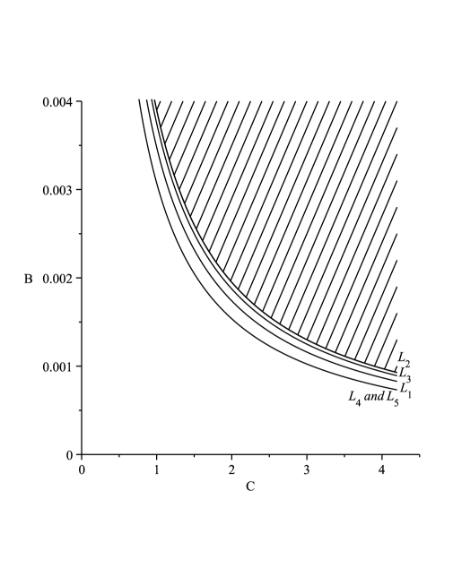
Figure 1: The stable region (hatched) and the boundaries $(L_{1},L_{2},L_{3},L_{4}\,and\,L_{5})$ of different topological types of the regions of the possible motion for $\displaystyle\frac{m_{1}}{9}=\frac{m_{2}}{3}=\frac{m_{3}}{1}$.

Knowing the coordinates of singular points and constant $C$, from formula (7) the values of Sundman constant $B_{1},B_{2},B_{3}$ and $B_{4,5}$ in all singular points $L_{i},(i=1,2,\dots,5)$ are calculated. Constants $C$ and $B_{i}$ are connected by reciprocal proportion

$$B_{i}=\frac{G^{2}}{4mC}\Bigl{[}m_{1}m_{2}+m_{2}m_{3}(r_{23}^{2})_{i}+m_{3}m_{1}(r_{31}^{2})_{i}\Bigl{]}\left[m_{1}m_{2}+\frac{m_{2}m_{3}}{(r_{23})_{i}}+\frac{m_{3}m_{1}}{(r_{31})_{i}}\right]^{2},$$ (16)

where $(r_{23})_{i}$ and $(r_{31})_{i}$ are calculated at the singular point $L_{i}$.

The relations (16) have been established by Golubev (1967) in the $c^{2}h$ method.

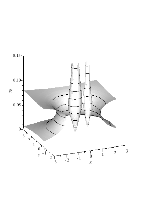
Figure 2: General view of Sundman surfaces for $\displaystyle\frac{m_{1}}{9}=\frac{m_{2}}{3}=\frac{m_{3}}{1}$, $C$=2 and $B=B_{2}$. Surfaces are represented in the field of the space limited to planes: $x=-3,\,x=3,\,y=-1,\,y=3,\,R=0,\,R=0.7$.

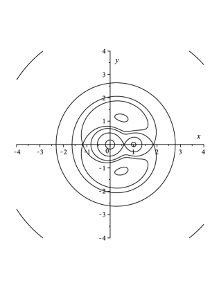
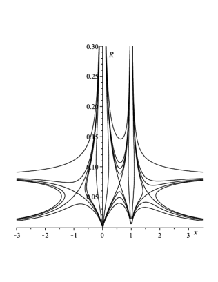
Figure 3: The sections of the Sundman surfaces for $\displaystyle\frac{m_{1}}{9}=\frac{m_{2}}{3}=\frac{m_{3}}{1}$ by the plane $R=R_{2}$ (left), by the plane $y=0$ (right).

Singular points are the points of bifurcation, in which a qualitative change in the shape of Sundman surface occurs. The curves (16) on plane $CB$ are the boundaries of the topologically different regions of the possible motion. The curve $L_{2}$ limits the Sundman stable region of the body $M_{3}$, and this stable region is shaded (Fig.1).

The general form of the Sundman surfaces for three bodies with the mass ratio proportional to 9:3:1 is shown in Fig.2; the section of the Sundman surfaces by the planes $R=R_{2}$ and $y=0$ is presented in Fig.3.

In the general three-body problem, as in the restricted problem, the concept of Hill stability is conserved. But, to distinguish it from the restricted problem in the general three-body problem, we will call this stability Sundman stability.

We will call the motion of the body $M_{3}$ in the general three-body problem stable on Sundman if there are such regions of the possible motions, limited by the appropriate Sundman surfaces, inside which the body $M_{3}$ will be always (at any instant of time) located at a finite distance from one of the bodies $M_{1}$ or $M_{2}$. In other words, the body $M_{3}$ will be an eternal satellite of one of $M_{1}$ or $M_{2}$ bodies, while bodies $M_{1}$ or $M_{2}$ can be at any distance one from the other, including infinite.

Criterion of Sundman stability is the inequality

$$B\geq B_{2},$$ (17)

where $B_{2}$ is the value of Sundman constant in the inner Euler libration point $L_{2}$. The fulfillment of this condition guarantees that the body $M_{3}$ can be: in some ”spindly” surfaces (see Fig.2, 3) remaining the eternal satellite of a body $M_{1}$; or in other ”spindly” surfaces, remaining the satellite of body $M_{2}$, or in a remote open oval area, when the distance between bodies $M_{1}$ and $M_{2}$ remains finite, not exceeding $Gm_{1}m_{2}/C$. This last case can be treated as Sundman stability of the relative motion of bodies $M_{1}$ and $M_{2}$.

Thus, for (17) any pair of bodies will have Sundman stability if at the initial instant the bodies forming this pair are in one of these regions of stability. The loss of stability (body $M_{3}$ leaving the ”spindly” area) occurs if the value $R$ is close enough to its value $R_{2}$ at the libration point $L_{2}$.

3 SUNDMAN STABILITY
OF THE PLANET SATELLITES’ MOTION

The analysis of Sundman stability of the motion of all known natural planet satellites of the Solar System is investigated with the presented theory. The ephemeris of all planet satellites are calculated with the most uptodate theories implemented on the NSDC web-site (Natural Satellites Data Center) (Sternberg Astronomical Institute, Moscow, Russia), constructed by Emelyanov, Arlo (2008) $(http://www.sai.msu.ru/neb/nss/index.htm)$. From these ephemeris constants $C$, $B$ and $B_{2}$ were calculated in the barycentric coordinate system. Sundman stability was determined from formula (17).

For each satellite the construction of the Sundman surface sections by the coordinate plane $xy$ was also conducted. The sections are given for the Jovian satellite J6 Himalia and J9 Sinope (Fig.4). Himalia’s Sundman curve is within the Sundman stability region, Sinope’s curve is outside. In spite of the location of the Sinope orbit inside the Sundman lobe, which corresponds to Sundman constant value $B=B_{2}$, its energy is sufficiently high, and it has a potential capability to leave this lobe (see the dash curve). But this does not mean that the satellite will leave the vicinity of the planet without fail. Sundman instability means that the Sundman surfaces are open and allow it to leave the vicinity of planet. But the Sundman surfaces do not tell if this will occur or not. The same case is for the Hill stability.

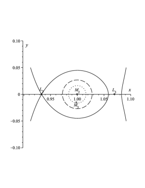
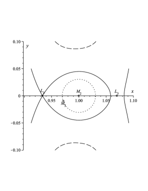
Figure 4: The sections of the Sundman surfaces by the plane of $R=R_{2}$ for Jovian satellites J6 Himalia (left) and J9 Sinope (right). Here: the solid line $B_{2}$ is the boundary of Sundman stability region, the dash line is satellite’s Sundman curve, the dotted line is approximate region of satellite motions.

Lukyanov (2011) showed the Sundman stability of the Moon motion. The Sundman stability results for the rest satellites are given in Tables (1-5). The tables also list the results of the classical Hill stability. All satellites are located in the order of increasing semimajor axes of their orbits around the planet. The relative masses of distant planet satellites obtained from satellite photometric observations (Emelyanov, Uralskaya, 2011), are taken from the web-site NSDC (http://www.sai.msu.ru/neb/nss/index.htm).

The Martian satellites (Phobos and Deimos) have Hill and Sundman stability (Tab.1).

The main and the inner satellites of Jupiter have Hill stability and Sundman stability and are not included in the tables. The distant satellites, which have prograde and retrograde orbits, are of special interest. All prograde satellites of Jupiter have Hill and Sundman stability (Tab.LABEL:Tab1). All retrograde satellites with $a>18.34\cdot 10^{6}\,km$ are unstable according to Hill and Sundman, independently from their masses. An exception is the satellite S/2003 J12 ($a=19\cdot 10^{6}\,km$, $i=145.8^{o}$, $e=0.376$) with a relatively small mass, which has Hill stability and Sundman stability.

The situation is different for the satellites of Saturn. The main, inner and distant prograde satellites of Saturn, which belong to the Gallic group ($i=34^{o}$) and Inuit group ($i=45^{o}$), have Hill stability and Sundman stability (Tab. 3). The retrograde satellites with $a<18.6\cdot 10^{6}\,km$ have Hill and Sundman stability, with $a>18.6\cdot 10^{6}\,km$ have Hill stability, but Sundman instability. Furthermore, Sundman unstable is also the satellite S LI Greip with the semimajor axis $a=18.1\cdot 10^{6}\,km$.

The main and inner satellites of Uranus have the Hill stability and Sundman stability. The stability results coincide for all distant satellites, except for the most distant satellite U XXIV Ferdinand ($a=20.9\cdot 10^{6}\,km$), which has Sundman instability (Tab.4).

Triton and the Neptune inner satellites have the Hill and Sundman stability. Two distant Neptune satellites have Sundman instability: N X Psamathe ($a=46\cdot 10^{6}\,km$) and N XIII Neso ($a=48\cdot 10^{6}\,km$). The rest of Neptune satellites have Hill stability and Sundman stability (Tab.5).

The comparison of the results of the Sundman stability and Hill stability shows that Hill stability always follows from the Sundman stability, but the reverse assertion is not correct. It is caused by the fact that, in contrast to Hill’s model, in the Sundman model the satellite masses are not zero, but are finite. Therefore, each satellite of any planet has an individual value of the Sundman constant $B_{2}$, while in Hill’s model all satellites of any planet have the same value of the Hill constant $C_{2}$.

The comparison of the obtained results with Golubev $c^{2}h$ method is carried out in two directions:

— comparison of the stability criteria used,

— comparison of the obtained regions of the possible motions.

Analytical forms of stability criterion in our work $B\geq B_{2}$ and in Golubev’s method $c^{2}h\leq(c^{2}h)_{cr}$, are the same. But the calculation of the constants in the left and right sides of the inequalities is carried out using different formulas. This leads to some differences in numerical results. The comparison with the results of the work (Walker et al, 1980) for the satellites J1-J13 shows that the Sundman stability or instability of the these satellites, obtained in our work, agrees with the results of Walker et al. (1980) for all satellites, except for four satellites of Jupiter with retrograde motion, J VIII, J IX, J XI and J XII. For these satellites we obtained instability, while in the work cited these satellites were indicated as being stable. This is likely to be due to the approximation of the three-body problem by two problem of two bodies and also by the neglect of orbit inclinations.

We conducted the construction of regions of possible motions in the three-dimensional space of $xyR$, while in all works of other authors the value of $R$ is excluded from the examination, and the constructions of regions of possible motions are conducted in the $xy$-plane. For this reason in the $c^{2}h$ method it is not possible to get a number of important results. For example, it cannot be obtained that the loss of stability (withdrawal of the body $M_{3}$ from the stability region) can occur only for a certain distance between the bodies $M_{1}$ and $M_{2}$. Generally, Sundman curves in the plane $R=\mathrm{const}$ with a change in $R$ can sharply and qualitatively differ from Hill’s curves, as shown by Lukyanov (2011).

4 DISCUSSION

The famous Sundman inequality in the general three-body problem takes the form

$$(U-C)J-B\geq\frac{\dot{J}^{2}}{8}.$$ (18)

For the material motions of bodies, i.e., with the fulfillment of conditions $\dot{J}^{2}\geq 0$, it determines the regions of possible motions satisfying the inequality

$$(U-C)J\geq B.$$ (19)

The boundaries of the region of possible motions are determined by the equation

$$(U-C)J=B,$$ (20)

which we call the equation of the Sundman surface, while the stability in Hill’s sense for the three-body problem — Sundman stability. By analogy with the surfaces of the zero speed in the restricted three-body problem, we may call the Sundman surfaces in the general three-body problem the surfaces of zero rate of change of the barycentric moment of inertia of bodies $(\dot{J}=0)$.

The determination of the Sundman stability and the construction of the Sundman curves in the plane of parameters $C$ and $B$ (see Fig. 1) is completely solved by Golubev (1967) in his $c^{2}h$ method (in our designations $c^{2}=2B,h=-C$). Now this method is called Golubev’s method.

Golubev’s method determines not the surfaces, but the Sundman curves located in the plane of the triangle formed by the mutual distances between the bodies. The mutual distances between the bodies $R_{13}$ and $R_{23}$ are substituted by the relative values $R_{13}/R$ and $R_{23}/R$, and the value of $R=R_{12}$ is generally excluded from examination.

Equation of ”current” Sundman curve in Golubev’s method has the form of the hyperbola $CB=\mathrm{const}$. If in this case the constants $C$ and $B$ are expressed in term of any other variables, then, in its turn, the task of construction of the Sundman curves in the space of these variables arises. Thus, in the large series of works of (Szebehely and Zare, 1976), (Walker, 1983), (Donnison, 2010) and many other authors the task of constructing Hill-Sundman curves and determination of stability regions in the general three-body problem is solved by Golubev’s method in the space of six quantities: semimajor axes $a_{1},a_{2}$, eccentricities $e_{1},e_{2}$ and inclinations $i_{1},i_{2}$, for calculation of the constants $C$ and $B$ the approximation of three-body problem by two problems of two bodies is used. This introduces a certain error to the solution of problem. Besides, the value of $R$ remains unknown.

For the representation of the Sundman curves on the plane $xy$, Golubev (1968) considered another method. He used the simplified Sundman inequality instead of the exact inequality (19)

$$U^{2}J\geq BC,$$ (21)

which is the consequence of inequality (19) and is obtained after the multiplication of inequality (19) by $U$, taking into account inequalities $C>0$ and $U>C$. Inequality (21) does not reflect the entire diversity of the Sundman surfaces.

Like the $c^{2}h$ criterion (obtained from the condition of the positivity of the discriminant of the quadratic trinomial for $R$ from the left side of the Sundman inequality), simplified inequality (21) does not contain the mutual distance $R_{12}=R$. Therefore, by means of inequality (21), it is possible to construct not the surfaces, but the Sundman curves in the plane of relative coordinates $xy$. The construction of these curves was subsequently conducted in the works of (Marchal, Saari, 1975), (Marchal, Bozis, 1982) and other authors.

Thus, the task of constructing the Sundman surfaces in the space of the coordinates used remained incomplete before the publication (Lukyanov, Shirmin, 2007) and (Lukyanov, 2011) appeared. Lukyanov, Shirmin (2007) used the mutual distances between the bodies as the coordinates. This made possible to construct exact Sundman surfaces in the three-dimensional space of mutual distances. Lukyanov (2011) used the more convenient rectangular coordinate system $xyR$, determined by the accompanying triangle of mutual positions of three bodies.

In these works the exact Sundman inequality (19) is used and, therefore, the value of $R$ is not excluded from the examination. In this case no simplifications or assumptions are applied. The construction of the Sundman surfaces is implemented in the three-dimensional space of the coordinates used with the determination of the singular points of surfaces, regions of the possible motion and Sundman stability regions.

Regions of the possible motion constructed by means of the exact Sundman inequalities differ from analogous regions defined according to the simplified Sundman inequality, both quantitatively and qualitatively.

The stability regions determined by the simplified Sundman inequality (21) have larger sizes than those calculated by exact inequality (19). Therefore, the stability obtained by means of (21) can turn to instability, when using exact inequality (19).

It is easy to derive by means of the exact Sundman surfaces that the loss of Sundman stability for the body $M_{3}$ can occur only when a certain distance $R$ between the bodies $M_{1}$ and $M_{2}$ takes place, so that the ”passage” through the neighborhood of the singular point $L_{2}$ is open. It is caused by the fact that the singular points of the Sundman surfaces are determined by three coordinates $L_{i}(x_{i},y_{i},R_{i})$ and in the space $xyR$ they lie, generally speaking, in different planes. This result cannot be established with the aid of inequality (21), since it does not depend on $R$.

The construction of exact Sundman surfaces allows us to define the regions of possible motions for any of the three bodies and for any values of $C$ and $B$. Using the Sundman surfaces yields, for example, that with the fulfillment of the stability criterion the body $M_{3}$ (it can be any body) for any time $-\infty<t<\infty$ will be located at a finite distance from one of the bodies $M_{1}$ or $M_{2}$ or at a large distance from these bodies. Qualitatively, the analogous result is known for the Hill surfaces in the restricted three-body problem as well. If the body $M_{3}$ is located, for example, in the stability region near $M_{1}$, then the Sundman surfaces admit the possibility of retreating of the body $M_{2}$ to any large distance from the pair $M_{1},M_{3}$. For the Hill surfaces this situation is not possible.

By means of the Sundman surfaces it is possible to establish the stability of only one pair of bodies, and the third body will be in this case unstable in the Sundman sense. Sundman surfaces do not establish the simultaneous stability of three bodies, i.e., guaranteed location of all bodies in a certain finite region of the space (Lagrange stability), although these surfaces do not exclude this case. Sundman instability does not mean that a body will necessarily leave the neighborhood of another body. The Sundman surfaces do not allow us to determine if this retreat will actually occur. This result is analogous to that of Hill stability. The determination of Sundman stability of the planet satellites of the Solar system conducted in this study shows the effectiveness of the use of Sundman surfaces in the coordinate form.

We believe that our results represent a certain interest for celestial mechanics and for astronomy as a whole.

Table 1: Martian satellites. Here $a$ is the semimajor axis of the satellite orbit, $i$ is the inclination, $e$ is the eccentricity, $m/M_{P}$ is the ratio of the satellite mass to the planet mass.

Satellite	$a$	$e$	$i$	$m/M_{P}$	Stability
	($km$)		($deg$)	$10^{-8}$	Hill	Sundman
M1 Phobos	9380	0.0151	1.1	1.6723	yes	yes
M2 Deimos	23460	0.0002	0.9 – 2.7	0.2288	yes	yes

Table 2: The irregular Jovian satellites

(the notation in Table 1).
Satellite	$a$	$i$	$e$	$m/M_{P}$	Stability
	$(10^{6}km$)	($deg$)		$10^{-9}$	Hill	Sundman
1	2	3	4	5	6	7
XVIII Themisto	7.507	43.08	0.242	3.4889	yes	yes
XIII Leda	11.165	27.46	0.164	5.76	yes	yes
VI Himalia	11.461	27.50	0.162	22101.8	yes	yes
X Lysithea	11.717	28.30	0.112	331.5	yes	yes
VII Elara	11.741	26.63	0.217	4578.2	yes	yes
XLVI Carpo	16.989	51.4	0.430	0.3394	yes	yes
S/2003 J3	18.340	143.7	0.241	0.1263	no	no
S/2003 J12	19.002	145.8	0.376	0.0631	yes	yes
XXXIV Euporie	19.302	145.8	0.144	0.2447	no	no
S/2003 J18	20.700	146.5	0.119	0.2920	no	no
XXXV Orthosie	20.721	145.9	0.281	0.3315	no	no
XXXIII Euanthe	20.799	148.9	0.232	0.4341	no	no
XXIX Thyone	20.940	148.5	0.229	0.6946	no	no
S/2003 J16	21.000	148.6	0.270	0.1342	no	no
XL Mneme	21.069	148.6	0.227	0.3315	no	no
XXII Harpalyke	21.105	148.6	0.226	0.8367	no	no
XXX Hermippe	21.131	150.7	0.210	1.4919	no	no
XXVII Praxidike	21.147	149.0	0.230	2.8495	no	no
XLII Thelxinoe	21.162	151.4	0.221	0.3473	no	no
XXIV Iocaste	21.269	149.4	0.216	1.3971	no	no
XII Ananke	21.276	148.9	0.244	157.9	no	no
S/2003 J15	22.000	140.8	0.110	0.1342	no	no
S/2003 J4	23.258	144.9	0.204	0.0947	no	no
L Herse	22.000	163.7	0.190	0.2526	no	no
S/2003 J9	22.442	164.5	0.269	0.0947	no	no
S/2003 J19	22.800	162.9	0.334	0.1263	no	no
XLIII Arche	22.931	165.0	0.259	0.2842	no	no
XXXVIII Pasithee	23.096	165.1	0.267	0.1658	no	no
XXI Chaldene	23.179	165.2	0.251	0.7499	no	no
XXXVII Kale	23.217	165.0	0.260	0.2447	no	no
XXVI Isonoe	23.217	165.2	0.246	0.6157	no	no
XXXI Aitne	23.231	165.1	0.264	0.4026	no	no
XXV Erinome	23.279	164.9	0.266	0.3789	no	no
XX Taygete	23.360	165.2	0.252	1.1445	no	no
XI Carme	23.404	164.9	0.253	694.6	no	no
XXIII Kalyke	23.583	165.2	0.245	1.5471	no	no
XLVII Eukelade	23.661	165.5	0.272	0.7104	no	no
XLIV Kallichore	24.043	165.5	0.264	0.2289	no	no
S/2003 J5	24.084	165.0	0.210	0.9788	no	no
S/2003 J10	24.250	164.1	0.214	0.0947	no	no
XLV Helike	21.263	154.8	0.156	0.7183	no	no
XXXII Eurydome	22.865	150.3	0.276	0.4262	no	no
XXVIII Autonoe	23.039	152.9	0.334	0.7814	no	no
XXXVI Sponde	23.487	151.0	0.312	0.2763	no	no
VIII Pasiphae	23.624	151.4	0.409	1578.7	no	no
XIX Megaclite	23.806	152.8	0.421	2.1312	no	no
IX Sinope	23.939	158.1	0.250	394.7	no	no
XXXIX Hegemone	23.947	155.2	0.328	0.3394	no	no
XLI Aoede	23.981	158.3	0.432	0.6473	no	no
S/2003 J23	24.055	149.2	0.309	0.0947	no	no
XVII Callirrhoe	24.102	147.1	0.283	5.3044	no	no
XLVIII Cyllene	24.349	149.3	0.319	0.2368	no	no
XLIX Kore	24.543	145.0	0.325	0.3947	no	no
S/2003 J2	28.570	151.8	0.380	0.1500	no	no

Table 3: The irregular Saturnian satellites (the notation in Table 1).

Satellite	$a$	$i$	$e$	$m/M_{P}$	Stability
	($10^{6}km$)	($deg$)		$10^{-11}$	Hill	Sundman
XXIV Kiviuq	11.111	45.71	0.334	0.8629	yes	yes
XXII Ijiraq	11.124	46.44	0.316	0.3248	yes	yes
IX Phoebe	12.944	174.8	0.164	1458.957	yes	yes
XX Paaliaq	15.200	45.13	0.364	2.2728	yes	yes
XXVII Skathi	15.541	152.6	0.270	0.0588	yes	yes
XXVI Albiorix	16.182	33.98	0.478	4.3629	yes	yes
S/2007 S2	16.560	176.7	0.218	0.0248	yes	yes
XXXVII Bebhionn	17.119	35.01	0.469	0.0261	yes	yes
XXVIII Erriapus	17.343	34.62	0.474	0.2294	yes	yes
XXIX Siarnaq	17.531	45.56	0.295	24.1988	yes	yes
XLVII Skoll	17.665	161.2	0.464	0.0237	yes	yes
LII Tarqeq	17.920	49.86	0.107	0.0385	yes	yes
XXI Tarvos	17.983	33.82	0.531	0.5455	yes	yes
LI Greip	18.105	172.7	0.374	0.0158	yes	no
XLIV Hirrokkin	18.437	151.4	0.333	0.0965	yes	yes
S/2004 S13	18.450	167.4	0.273	0.0148	yes	yes
S/2004 S17	18.600	166.6	0.259	0.0082	yes	yes
L Jarnsaxa	18.600	162.9	0.192	0.0116	yes	no
XXV Mundilfari	18.685	167.3	0.210	0.0464	yes	no
S/2006 S1	18.981	154.2	0.130	0.0192	yes	no
XXXI Narvi	19.007	145.8	0.431	0.0340	yes	no
XXXVIII Bergelmir	19.338	158.5	0.142	0.0248	yes	no
XXIII Suttungr	19.459	175.8	0.114	0.0422	yes	no
S/2004 S12	19.650	164.0	0.401	0.0142	yes	no
S/2004 S07	19.800	165.1	0.580	0.0200	yes	no
XLIII Hati	19.856	165.8	0.372	0.0185	yes	no
XXXIX Bestla	20.129	145.2	0.521	0.0432	yes	no
XL Farbauti	20.390	156.4	0.206	0.0113	yes	no
XXX Thrymr	20.474	176.0	0.470	0.8278	yes	no
S/2007 S3	20.518	177.2	0.130	0.0119	yes	no
XXXVI Aegir	20.735	166.7	0.252	0.0214	yes	no
S/2006 S3	21.132	150.8	0.471	0.0100	yes	no
XLV Kari	22.118	156.3	0.478	0.0409	yes	no
XLI Fenrir	22.453	164.9	0.136	0.0095	yes	no
XLVIII Surt	22.707	177.5	0.451	0.0127	yes	no
XIX Ymir	23.040	173.1	0.335	1.3878	yes	no
XLVI Loge	23.065	167.9	0.187	0.0232	yes	no
XLII Fornjot	25.108	170.4	0.206	0.0211	yes	no

Table 4: The irregular Uranus’ satellites (the notation in Table 1).

Satellite	$a$	$e$	$i$	$m/M_{P}$	Stability
	$(10^{6}km$)		($deg$)	$10^{-9}$	Hill	Sundman
XXII Francisco	4.2760	0.1425	147.613	0.0658	yes	yes
XVI Caliban	7.1689	0.0823	139.681	8.1305	yes	yes
XX Stephano	7.9424	0.1459	141.538	0.3494	yes	yes
XXI Trinculo	8.5040	0.2078	166.332	0.0593	yes	yes
XVII Sycorax	12.2136	0.5094	152.669	46.6790	yes	yes
XXIII Margaret	14.3450	0.7827	50.651	0.0609	yes	yes
XVIII Prospero	16.1135	0.3274	146.340	1.1306	yes	yes
XIX Setebos	18.2052	0.4943	148.828	1.4240	yes	yes
XXIV Ferdinand	20.9010	0.4262	167.278	0.0874	yes	no

Table 5: The irregular Neptune’s satellites (the notation in Table 1).

Satellite	$a$	$e$	$i$	$m/M_{P}$	Stability
	$(10^{6}km$)		($deg$)	$10^{-9}$	Hill	Sundman
II Nereid	5.5134	0.7512	7.232	301.38	yes	yes
IX Halimede	15.728	0.5711	134.101	3.0835	yes	yes
XI Sao	22.422	0.2931	48.511	0.6445	yes.	yes
XII Laomedeia	23.571	0.4237	34.741	0.5606	yes	yes
X Psamathe	46.695	0.4499	137.391	0.9244	yes	no
XIII Neso	48.387	0.4945	132.585	1.3423	yes	no

REFERENCES

Donnison J.R., Williams I.P., 1983, Celest. Mech., 31, 123.

Donnison J.R., 2009, Planet. Space Sci., 57, 771.

Donnison J.R., 2010, Planet. Space Sci., 58, 1169.

Emel’yanov N.V., Arlot J.-E., 2008, Astron. Astrophys., 487, 759.

Emelyanov N.V., Uralskaya V.S., 2011, Solar Syst. Res., 45, 5, 377.

Golubev V.G., 1967, Doklady. Akad. Nauk SSSR, 174, 767.

Golubev V.G., 1968, Sov. Phys. Dokl., 13, 373.

Golubev V.G., Grebenikov E.A., 1985, The three-body problem in Celestial Mechanics, Moscow University Publisher, Moscow (in russian).

Hagihara Y., 1952, Japan Academy, 28, Number 2.

Hill G.W., 1878, Am. J. Math., 1, 5.

Li J., Fu Y., Sun Y., 2010, Celest. Mech. Dynam. Astron., 107, 21.

Lukyanov L.G., Shirmin G.I., 2007, Astr. Letters, 33, 550.

Lukyanov L.G., 2011, Astron. Rep., 55, 742.

Marchal C., Saari D., 1975, Celest. Mech., 12, 115.

Marchal C., Bozis G., 1982, Celest. Mech., 26, 311.

Marchal C., 1990, The Three-Body Problem, Elsevier Publisher, Amsterdam.

Natural Satellites Data Center (NSDC)
($http://www.sai.msu.ru/neb/nss/index.htm$)

Proskurin V.F., 1950, Bull. Inst. Theor. Astr., IV, Number 7, 60.

Sundman K.F., 1912, Acta Math., 36, 195.

Szebehely V., Zare K., 1977, Astron. Astrophys, 58, 145.

Walker I.W., Emslie A.G., Roy A.E., 1980, Celest. Mech., 22, 371.

Zare K., 1976, Celest. Mech., 14, 73.