Ground state and excitation spectra of a strongly correlated lattice by the coupled cluster method.

Abstract

We apply Coupled Cluster Method to a strongly correlated lattice Hamiltonian and we extend the Coupled Cluster linear response method to the calculation of electronic spectra. We do so by finding an approximation to a resolvent operator which describes the spectral response of the Coupled Cluster solution to excitation operators. In our Spectral Coupled Cluster Method the ground and excited states appear as resonances in the spectra and the resolvent can be iteratively improved in selected spectral regions. We apply our method to a $MnO_{2}$ plane model which corresponds to previous experimental works.

1 Introduction

The numerical methods for solid state physics span a wide range of techniques which aim to provide approximate solutions to the problem of many body interactions in correlated systems; the exact solution being unknown. Between these techniques some of the most notables are: the DMF theory, which uses a self-energy correction term obtained from an Anderson impurity many-body solution, the GW equation, which calculates the self-energy with neglection of vertex corrections, the quantum monte-carlo method and the Coupled-Cluster Method (CCM). The Coupled-Cluster method has been conceived in the $50s$ by Fritz Coester and Hermann Kummel for nuclear physics, and has since progressively gained other domains[1]. In quantum-chemistry, in particular, CCM is widely regarded as the most reliable choice when high accuracy is needed[2]. Concerning the lattice models of strongly interacting electrons CCM has recently been applied to spin lattices[3] and to Hubbard model[4].

Although the CCM was initially formulated as a ground state approximation, the recent developpment of CCM time dependent linear response [5] has stretched the CCM applicability to excited states. In particular Crawford and Ruud have calculated vibrational eigenstates contributions to Raman optical activity[6] while Govind et al. have calculated excitonic states in potassium bromide[7].

In this paper we extend the coupled cluster linear response method to the calculation of electronic excitation spectra. To do so we represent an initial wave-function as the product of the probe operator times the CCM solution, and we develop an original solution method of the resolvent equation for the CCM ansatz.

This paper is organised in the following way. In section 2 we detail the equations. In section 3 we describe the model of a $MnO_{2}$ plane derived from previous absorption and scattering x-ray spectroscopy studies, on which we test our method. We discuss the results of our Spectral Coupled Cluster Method in section 4. There we also validate the method by comparing it to the exact solution that we can obtain when we restrict the Hilbert space dimension to such an extent that the exact diagonalisation is possible.

2 Method

In the Coupled-Cluster method[1] one searches an approximated solution to the eigen-problem

$$H\left|\Psi\right>=E\left|\Psi\right>$$ (1)

where $H$ is the Hamiltonian in second quantization and is formed by a sum of products of one-particle creation and annihilation operators. The one-particle operators change, between $1$ and $0$, the occupation integer number of the one-particle orbitals contained in the model.

The solution is represented, given a reference state $\left|\Phi_{0}\right>$, by the exponential ansatz

$$\left|\Psi\right>=e^{S}\left|\Phi_{0}\right>\simeq e^{S_{N}}\left|\Phi_{0}\right>$$ (2)

where $S$ is the ideal exact solution and $S_{N}$ is a sum, truncated to $N$ terms, of products of electron-hole pair excitations :

$$S_{N}=\sum^{N}_{i=1}{t_{i}~{}Symm{\left\{\prod_{k=1}^{n_{i}}c^{\dagger}_{\alpha_{i,k}}c^{\dagger}_{a_{i,k}}\right\}}}$$ (3)

In this formula $N$ is the number of degrees of freedom of the ansatz. The larger is this number the more accurate is the representation. The $t_{i}$’s are free coefficients that must be obtained from the CCM equations below. Each term in the sum is the product of a set of electron(hole)-creation operators $c^{\dagger}$. Each term is determined by a choice of indexes $\alpha_{i,k}$( $a_{i,k}$), with the greek(latin) letter $\alpha$(a) ranging over empty(occupied) orbitals. One can cosiders the reference state as the vacuum state and that each term $i$ in the sum $S_{N}$ creates, from vacuum, an excited state which is populated by $n_{i}$ particles (holes and/or electrons). The $Symm$ operator makes the ansatz symmetric for the Hamiltonian symmetry subgroup which transforms, up to a factor, the reference state $\left|\Phi_{0}\right>$ into itself.

In the Coupled Cluster method, the rationale for the exponential ansatz resides in its size extensivity property. This means that for a system composed of two non correlated parts, $A$ and $B$, the coupled cluster ansatz operator can be factorized as the product of two operators $e^{S^{A+B}}=e^{S^{A}}e^{S^{B}}$. This simple factorisability relation has deep consequences[1], whose one of the most important is that, in a system with periodic translational symmetry, the calculation complexity for a given accuracy does not depends on the system size.

The CCM equations are obtained substituting $\left|\Psi\right>$, in the eigen-equation, with its ansatz and by multiplying at the left with $e^{-S_{N}}$, the inverse of the ansatz operator . One obtains for the eigenvalue

$$E=\left<\Phi_{0}\right|e^{-S_{N}}He^{S_{N}}\left|\Phi_{0}\right>$$ (4)

while the free parameters are obtained setting the eigen-equation residue to zero in the space of excited states which enter the $S_{N}$ sum :

$$0=\left<\Phi_{0}\right|\left(\prod_{k=1}^{n_{i}}c_{a_{i,k}}c_{\alpha_{i,k}}\right)e^{-S_{N}}He^{S_{N}}\left|\Phi_{0}\right>~{}\forall i\in[1,N]$$ (5)

The Coupled Cluster Method expands these equations by means of the Hausdorff expansion formula which for two arbitrary operators $A$ and $B$ states that:

$$e^{-A}Be^{A}=B+[B,A]+1/2[[B,A],A]+..1/n![[B,A]...],A]+...$$ (6)

The numerical applicability of CCM relies on the fact that, when $A$ is substituted with $S_{N}$ and $H$ replaces $B$, only the first five terms in the series, can be non zero. This can be demonstrated considering that $S_{N}$ is formed by creation operators only, and that the interactions contained $H$ are composed by products of up to four single-particle operators for the Coulomb interaction. For each term of the expansion every $S_{N}$ entering in the commutators must have at least one one-particle creation operator contracted with one annihilation operator of $H$, for the term not to be identically zero.

Equation 5 gives $N$ polynomial equations by which we can determine the $N$ unknowns $t_{i}$. These equations have order up to the fourth in the $t_{i}$ variables because this is the maximum order in $S_{N}$ for the non-zero terms of the Hausdorff expansion.

The number of solutions of a system of polynomial equations explodes exponentially with the number of equations and it is not possible, except for small systems, to explore systematically the whole solutions space. To solve the equations, instead, we use the Newton’s method to follow the solution, increasing iteratively the number of free parameters and using as a starting point the for $N$ parameters the $N-1$ ones found at the previous iteration plus a random choice for the $N^{th}$ one.

The accuracy of the CCM solution increases with $N$. At each iteration the new $(N+1)^{th}$ term is constructed, in equation 3, by assigning its order $n_{(N+1)}$ and by choosing the concerned electron and hole orbitals which are expressed by the sets of indexes $\alpha_{(N+1),k}$ and $a_{(N+1),k}$, with $k$ ranging from $1$ to $n_{(N+1)}$ . We denote the ensemble of all possible choices with the symbol

$$\left\{\left(n^{\prime}_{\zeta},\alpha^{\prime}_{\zeta,1}...,a^{\prime}_{\zeta,1}...\right)\right\}$$ (7)

where the possible choices satisfy the condition

$$0\neq\left<\Phi_{0}\right|\left(\prod_{\zeta=1}^{n^{\prime}_{\zeta}}c_{a^{\prime}_{\zeta,k}}c_{\alpha^{\prime}_{\zeta,k}}\right)e^{-S}He^{S}\left|\Phi_{0}\right>$$ (8)

The simplest choice consists in choosing the $\zeta$ which gives the largest residue in equation 8.

Once we have obtained the CCM ground state and its ground energy $E$, we are interested in the transition probability for a time dependent perturbation $exp(i\omega_{D}t)D$, where $D$ is an arbitrary product of $c^{\dagger}$ operators. The transition rate is given by the Fermi golden rule which states that the probability for the absorption of an energy quantum $\hbar\omega_{D}=\hbar\omega-E$, with $\hbar\omega$ being the final state energy, is proportional to:

$$\rho_{D}(\omega,\gamma)=\Im m\frac{\left<\Phi_{0}\right|e^{S^{\dagger}}D^{\dagger}(H-\omega-i\gamma)^{-1}De^{S}\left|\Phi_{0}\right>}{\left<\Phi_{0}\right|e^{S^{\dagger}}e^{S}\left|\Phi_{0}\right>}$$ (9)

where $\gamma$ is a small line width. In order to calculate the above expression we have to solve two problems : find an approximate solution $R$ for the resolvent equation :

$$(H-\omega-i\gamma)|R>=De^{S}\left|\Phi_{0}\right>$$ (10)

and calculate the scalar product.

We represent an approximated solution for the resolvent, introducing the approximating operator $R_{D,\omega,\gamma}$ and the following ansatz which is similar to the ansatz for $S$ with the difference that it contains both annihilation and creation operators and that, in order to accede to the whole spectra, no symmetrization is done : :

$$|R>= R_{D,\omega,\gamma}De^{S}\left|\Phi_{0}\right>$$ (11)

$$R_{D,\omega,\gamma}= r^{0}_{D,\omega,\gamma}+\sum^{N^{r}}_{i=1}{r^{i}_{D,\omega,\gamma}\prod_{k=1}^{n^{r}_{i}}\hat{c}_{j_{i,k}}}$$ (12)

in this expression $r^{i}$ are free parameters and we have introduced the notation $\hat{c}$ to represent in a compact way both creation and annihilation operators. The definition of the $\hat{c}$ operator is, naming by $N_{orbs}$ the total number of represented orbitals (occupied and empty) :

$$\hat{c}_{j}=\left\{\begin{matrix}c^{\dagger}_{j}&j\in[1,N_{orbs}]\\ c_{j-N_{orbs}}&j\in[N_{orbs}+1,2*N_{orbs}]\end{matrix}\right|$$ (13)

We build our spectral CCM equations (SCCM equations) by multiplying at the left with $e^{-S_{N}}$, and by setting the residue to zero :

$$1= \left<\Phi_{0}\right|D^{\dagger}e^{-S}(H-\omega-i\gamma)R_{D,\omega,\gamma}De^{S}\left|\Phi_{0}\right>$$ (14)

$$0= \left<\Phi_{0}\right|D^{\dagger}\left(\prod_{k=1}^{n^{r}_{i}}\hat{c}_{j_{i,k}}\right)^{*}e^{-S}(H-\omega-i\gamma)R_{D,\omega,\gamma}De^{S}\left|\Phi_{0}\right>~{}\forall i\in[1,N^{r}]$$ (15)

Note that the validity of the above equations relies on the fact that $D$, being a product of $c^{\dagger}$ operators, commutes with $S$. These equations are expanded by the Hausdorff expansion formula substituting, in equation 6, $A$ with $S_{N}$ and $B$ with $(H-\omega-i\gamma)R_{D,\omega,\gamma}$. The Hausdorff expansion contains, also in this case, a finite number of non-zero terms because each term of the the resolvent operator , in equation 12, contains a finite number of annihilation operators while, as discussed above, each term of $H$ contains a maximum of four annihilation operators.

The expansion gives a set of linear equations for the $r$ parameters. The resolvent equation accuracy is improved by systematically increasing $N^{r}$, selecting, at each iteration, the set of numbers

$$\left\{\left(n^{r}_{{}_{N^{r}+1}},j_{{}_{N^{r}+1,0}},....,j_{{}_{N^{r}+1,n^{r}_{N^{r}+1}}}\right)\right\}$$ (16)

corresponding to the largest residue in the SCCM equations. When we calculate the residue we fix $\omega=\omega_{r}$ at the center of the spectral region of interest. Over the spectral region of interest the $r$ parameters are given by a linear algebra operations of the kind $r=(M_{1})^{-1}(M_{2}+\omega M_{3})$ where the $M$’s are matrices obtained from SCCM expansion. Once we know the $R$ operator we can calculate the spectra with the following equation :

$$\rho_{D}(\omega,\gamma)=\Im m\frac{\left<\Phi_{0}\right|e^{S^{\dagger}}D^{\dagger}R_{D,\omega,\gamma}De^{S}\left|\Phi_{0}\right>}{\left<\Phi_{0}\right|e^{S^{\dagger}}e^{S}\left|\Phi_{0}\right>}$$ (17)

This expression can be expanded using the Wick’s theorem and the linked-cluster theorem as already done by Sourav et al.[8]. Contracting in all possible ways the operators contained in $D^{\dagger}R_{D,\omega,\gamma}D$ with themselves one obtains sum of products of Green’s function of different orders. To simplify this we use the simplest approximation which consists in setting to zero all the connected Green’s function excepted the one-particle Green’s function :

$$G(j_{1},j_{2})=\frac{\left<\Phi_{0}\right|e^{S^{\dagger}}\hat{c}_{j_{1}}\hat{c}_{j_{2}}e^{S}\left|\Phi_{0}\right>}{\left<\Phi_{0}\right|e^{S^{\dagger}}e^{S}\left|\Phi_{0}\right>}$$ (18)

We expand this equation for $G$ using the Wick’s and the linked-cluster theorems. We obtain a hierarchical set of equations involving Green’s functions of arbitrary order. This expansion needs to be truncated choosing a closure relation. This closure relation is already provided by the choice that we have made setting to zero all the connected Green’s functions except the two points one. To obtain the Dyson equation for the Green’s function we proceed in the following way. Each time we contract a $\hat{c}$ operator with one of the terms contained in $S$, on the right, or with $S^{\dagger}$ on the left, a new vertex is obtained from which a number of new lines, equal to the term order minus one, are coming out. We consider all the combinatorial ways of contracting all these lines with themselves, except one branch which propagates further the Green’s function. This is the analogous of the Hartree-Fock approximation where two of the four legs of each Coulomb vertex are contracted with each other.

The Dyson equation is solved iteratively. The final result for the spectral function of equation 17 depends linearly on the parameters $r$, functions of $\omega$, and contain products of Green’s functions ( defined by equation 18). The spectral resonances positions depend on the $r$ parameters, which are found by the SCCM equation and whose behavior accounts for many-body correlations. The resonances intensities, instead, depend on our Hartree-Fock-like truncation which still accounts many-body interactions but in the mean-field approximation.

3 Model

In previous studies on manganites we applied exact diagonalisation, and Lanczos method, to the study of resonant X-ray scattering [9] at $L_{2}$,$L_{3}$ edges and $K_{\beta}$ fluorescence [10]. The spectroscopy data were modeled with a small planar cluster, described in second quantization. The model consisted of the central Mn atom open shells orbitals, plus some selected orbitals localised on the first neighbouring shell of oxygens atoms and Mn atoms. These studies revealed a pronounced O 2p character of the doped charge carriers, and the non-local nature of the forces governing the charge redistribution phenomena which are very important in these systems. The accounting of few extra orbitals from neighbouring shells, beside the resonating atom, is crucial in describing these phenomena but one rapidly ecounters the limit of the exponential growth of the Hilbert space dimension, when trying to extend the size of the cluster. To calculate the ground state and spectra of larger systems, while still keeping a good description of the many-body correlations, we have developed the methods described in this paper.

We will compare SCC method to exact numerical results that we will obtain in a truncated Hilbert space.. To keep the system numerically affordable for the exact diagonalisation technique we consider a small $2x2$ $MnO_{2}$ lattice with periodic boundary conditions. The Mn sites are placed at integer coordinates $(2i,2j)$ with $i$ and $j$ taking the values $0$ and $1$ , while the oxygen atoms are at positions $(2i+1,2j)$ and $(2i,2j+1)$. In order to limit to the maximum the dimension of the Hilbert space we restrict the degrees of freedom to those orbitals which are the most important for the physics of manganites. These are the $e_{g}$ $3d$ orbitals of $Mn$, namely the $x^{2}-y^{2}$ and $3z^{2}-r^{2}$ orbitals, and the $p$ oxygen orbitals which point toward $Mn$ sites. For oxygens we restrict to $p_{x}$ for the $(2i+1,2j)$ sites and $p_{y}$ at the $(2i,2j+1)$ sites. These are the oxygen orbitals which bridge the Mn sites along the $x$ and $y$ directions. The system Hamiltonian is composed of several terms ;

$$H=H_{bare}+H_{hop}+H^{Mn}_{U}+H^{Mn}_{J}+H^{O}_{U}$$ (19)

namely $H_{bare}$ which contains the one-particle energies of the orbitals, the hopping Hamiltonian $H_{hop}$ which moves electron between neighboring sites, the Hubbard correlations $H^{Mn}_{U}$, $H^{Mn}_{J}$ and $H^{O}_{U}$ for Manganese and Oxygen. The $H^{O}_{U}$ term is used because, applying exact diagonalisation, we truncate the Hilbert space by limiting the $p$ orbitals occupation numbers between $1$ and $2$. In the CC method, instead, we cannot truncate because this would destroy commutation relations. We have the possibility instead, in CCM, of choosing a high value of $U$ in the Hubbard correlation $H^{O}_{U}$ , in conjunction with the oxygen part of $H_{bare}$ to effectively limit the oxygen $p$ orbitals occupation numbers thus making the comparison, with the truncated model exact solution, possible.

The bare Hamiltonian is

$$H_{bare}=\sum_{i,j,g_{d},\sigma}\epsilon_{d,\sigma}~{}d^{\dagger}_{{}_{g_{d},\sigma,2i,2j}}d_{{}_{g_{d},\sigma,2i,2j}}+$$

$$(\epsilon_{p}-U_{p})\sum_{i,j,\sigma}\left(p^{\dagger}_{{}_{x,\sigma,2i+1,2j}}p_{{}_{x,\sigma,2i+1,2j}}+p^{\dagger}_{{}_{y,\sigma,2i,2j+1}}p_{{}_{y,\sigma,2i,2j+1}}\right)$$ (20)

where the $g_{d}$ index takes the values $g_{d}=x^{2}-y^{2},3z^{2}-r^{2}$, with $x,y$ being in plane and $z$ out of plane. The $Mn$ one-particle energies $\epsilon_{\sigma}$ are spin-dependent to take into account the mean-field exchange with the Mn $t_{2g}$ occupied orbitals ($xy,xz,yz$)( whose degrees of freedom are discarded from the model). The oxygen orbitals term takes into account the Hubbard coefficient $-U_{p}$ to compensate $H^{O}_{U}$ and favoring double and single occupations on oxygens.

The hopping term is

$$H_{hop}=t~{}\sum_{i,j,g_{d},\sigma}\sum_{s=\pm 1}s\left(f_{g_{d},x}p^{\dagger}_{{}_{x,\sigma,2i-s,2j}}d_{{}_{g_{d},\sigma,2i,2j}}+f_{g_{d},y}p^{\dagger}_{{}_{y,\sigma,2i,2j-s}}d_{{}_{g_{d},\sigma,2i,2j}}+c.c.\right)$$ (21)

where

$$f_{3z^{2}-r^{2},x}=f_{3z^{2}-r^{2},y}=1/2$$

$$-f_{x^{2}-y^{2},y}=f_{x^{2}-y^{2},x}=\sqrt{3}/2$$

The Coulomb intra-site repulsive interaction for $Mn$ is made by a part for an electron pair on the same orbital, and another part for two different orbitals :

$$H^{Mn}_{U}\sum_{i,j,g_{d}}U_{d}~{}n_{{}_{g_{d},\sigma=+\frac{1}{2},2i,2j}}n_{{}_{g_{d},\sigma=-\frac{1}{2},2i,2j}}+\sum_{i,j,\sigma_{1},\sigma_{2}}U^{\prime}_{d}~{}n_{{}_{3z^{2}-r^{2},\sigma_{1},2i,2j}}n_{{}_{x^{2}-y^{2},\sigma_{2},2i,2j}}$$ (22)

The Coulomb exchange for $e_{g}$ orbitals is

$$H^{Mn}_{J}=J_{d}~{}\sum_{i,j,\sigma_{1},\sigma_{2}}d^{\dagger}_{{}_{3z^{2}-r^{2},\sigma_{2},2i,2j}}d^{\dagger}_{{}_{x^{2}-y^{2},\sigma_{1},2i,2j}}d_{{}_{3z^{2}-r^{2},\sigma_{1},2i,2j}}d_{{}_{x^{2}-y^{2},\sigma_{2},2i,2j}}$$ (23)

while the $e_{g}$-$t_{2g}$ exchange is included as a mean-field term inside $H_{bare}$.

Finally the oxygen Hubbard term is

$$\sum_{i,j}U_{p}~{}\left(n_{{}_{p_{x},\sigma=+\frac{1}{2},2i+1,2j}}n_{{}_{p_{x},\sigma=-\frac{1}{2},2i+1,2j}}+n_{{}_{p_{y},\sigma=+\frac{1}{2},2i,2j+1}}n_{{}_{p_{y},\sigma=-\frac{1}{2},2i,2j+1}}+2\right)$$ (24)

The contributions of the terms factored by $U_{p}$, in the total Hamiltonian, is identically zero when we restrict the $n_{p}$ occupations between $1$ and $2$.

To fix the free parameters of the model we use knowledge from our previous work on manganites[9]. Parameters are given in $eV$ units. The effective Slater integrals used in that work correspond, in the present model, to $U_{d}=6.88$, $U^{\prime}_{d}=5.049$, $J_{d}=-0.917$. The exchange with occupied polarized $t_{2g}$ orbitals gives a $\simeq 2eV$ splitting between $\epsilon_{d,\sigma=-\frac{1}{2}}=2$ and $\epsilon_{d,\sigma=+\frac{1}{2}}=0$, in the case of ferromagnetic alignement. We use a hopping $t=1.8$ taken from our previous work[9]. The parameter $\epsilon_{p}$ controls the amount of charge back-donation from oxygen to manganese. The predominant $O$ $2p$ character of doped holes found in manganites [10] corresponds to a value $\epsilon_{p}$ which raises the bare oxygen orbitals energies above the bare Mn ones. The value of $\epsilon_{p}$ influences the average occupation of the $e_{g}$ orbitals. These occupancies match the ones found in the previous works for a value $\epsilon_{p}\simeq 2$.

4 Discussion

To find the CCM ground state and determine the resolvent equation we have adapted our $Hilbert++$ [11, 9] code. This code was originally created to calculate x-ray spectroscopies of small strongly correlated clusters by exact diagonalisation. It implements a second quantisation representation of operators and determinants. We have implemented automatic computing of commutators and automatic extension of the excitations set for CCM and for our SCC method.

The exact diagonalisation and the Lancsoz tridiagonalisation for spectra calculation are performed with $Hilbert++$. The code generates the Hilbert space by applying several times the Hamiltonian on a vector basis which is beforehand initialized with a seed state. In this seed state, the occupied spinorbitals are all the oxygen ones and, for ferromagnetic alignement on the $Mn$ sites, all the spinorbitals $3z^{2}-r^{2}$ with spin $\sigma=+1/2$ . This state is named, in the rest of this paper, nominal reference configuration. The configurations having one or more oxygen sites unoccupied , are discarded in the exact calculation. With this limitation on the configurations, the generated Hilbert space growths up to a dimension which is slightly less than $7$ millions.

To reproduce with the $CCM$ method the exact calculation done on the truncated space we set $U_{p}$ as high as $10^{2}eV$.

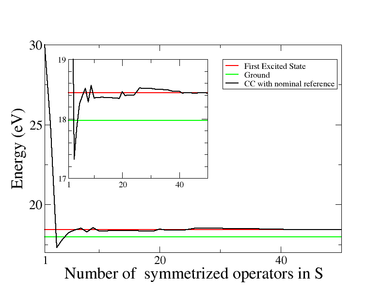
Figure 1: $CCM$ versus exact diagonalisation of the truncated Hilbert space space. For the $CCM$ method we apply an effective truncation by setting $U_{p}$ as high as $10^{2}eV$. The convergence of the $CCM$ energy is shown as a function of the number of symmetrized eccitations contained in the $S$ operator. The nominal reference generates the first excited state while the ground state has the symmetry of $\left|\hat{\Phi}_{0}\right>$, equation 25

We show in figure 1 the convergence of the $CCM$ energy as a function of the number of symmetrized eccitations contained in the $S$ operator when we take the nominal reference configuration as reference state The CCM energy converges, for the nominal reference, to the first excited eigenenergy, given by exact diagonalisation, above the ground state. We have analysed the ground and the first excited states that we obtain by exact diagonalisation. The largest component of the first excited state is found to be the nominal reference state. This explains why the CCM method, which takes this state as reference, converges to this eigen-state. The ground state, instead, has a different symmetry. We find that there are four components which have the largest factor and each of this component is obtained rotating the $e_{g}$ electron, on one of the four $Mn$ sites, from the $3z^{2}-r^{2}$ orbital to the $x^{2}-y^{2}$ one . More in details, the ground state has the same symmetry of the state $\left|\hat{\Phi}_{0}\right>$ given by

$$\left|\hat{\Phi}_{0}\right>=\sum_{i,j}(-1)^{i+j}d^{\dagger}_{{}_{x^{2}-y^{2},\sigma=1/2,2i,2j}}d_{{}_{3z^{2}-r^{2},\sigma=1/2,2i,2j}}\left|\hat{\Phi}_{0}\right>$$ (25)

This state cannot be obtained starting from the nominal reference with the $CC$ method because it has completely different symmetry properties. Notice for example that a $\pi/2$ rotation around the center of the cluster gives a factor $1$ if applied on the nominal reference but the same rotation gives a factor $-1$ when applied on $\left|\hat{\Phi}_{0}\right>$.

To force the $CC$ method to converge to such a symmetry state, a possible solution would be using the multi-reference $CC$ method. We have not implemented this method, which requires an a-priori knowledge of the solution, because our work is focussed on our Spectral Cluster Method that, as we will see in this section, is able to detect these states exploring selected spectral regions. To test further the capabilities of CCM to converge to the true ground state we have allowed a possible convergence to $\left|\hat{\Phi}_{0}\right>$ symmetry by using a reference state $\left|\bar{\Phi}_{0}\right>$ of lower symmetry :

$$\left|\bar{\Phi}_{0}\right>=d^{\dagger}_{{}_{x^{2}-y^{2},\sigma=1/2,0,0}}d_{{}_{3z^{2}-r^{2},\sigma=1/2,0,0}}\left|\Phi_{0}\right>$$ (26)

We show in figure 2 the convergence of the CCM energies for $U_{p}=5eV$ using two different choices of the reference state : the high symmetry state $\left|\Phi_{0}\right>$ and the lower symmetry $\left|\bar{\Phi}_{0}\right>$ . The CCM solution for reference state $\left|\bar{\Phi}_{0}\right>$ converges to a lower energy than the one obtained with the nominal reference state. We cannot compare this calculation, done with $U_{p}=5eV$, with the results of exact diagonalisation because the small value of $U_{p}$ gives access to a larger Hilbert space which is computationally more expensive. On the other hand for an high value of $U_{p}=10^{2}eV$, when comparaison with exact diagonalisation is possible, we have not been able to obtain the ground state starting from the low symmetry reference state $\left|\bar{\Phi}_{0}\right>$. We think that this difficulty can be explained in the following way : the lower energy of the $\left|\hat{\Phi}_{0}\right>$ symmetry state is due, in the $CCM$ equations, to a kind of bridges, made of operators which link the components of $\left|\hat{\Phi}_{0}\right>$ to each other. These bridges are created when an excitation operator, which composes $S$, is transformed by the Hausdorff commutation expansion into another excitation operator which will subsequently enter $S$, and so on. For the particular symmetry of $\left|\hat{\Phi}_{0}\right>$ to be obtained from $\left|\bar{\Phi}_{0}\right>$, these bridges must be long enough to transform one component into another. The problem of using a high value of $U_{p}$ is that for every pair of excitation operators which both create a hole on the same oxygen site, a new term coming from their product, will appear in the residue containing two holes that site. This will necessitate a new higher order excitation to be subsequently included in $S$ whose contributions will cancel the product of the two operators. This because the very high value of $U_{p}$ forbids double hole occupancies on oxygen sites. The need of accounting more operators requires more iterations. During these iteration the $\left|\hat{\Phi}_{0}\right>$ symmetry is non favorable and our procedure converges to higher eigenvalues. The CCM wavefunction corresponding to the true ground state becomes energetically favorable for a number of eccitation operators about $40$. The use of a multireference could have been used to force a particular symmetry. This procedure would have been feasible for the small system that we have treated in this work, because we can know the ground state symmetry from the exact solution. For larger systems, however, even if one could a-priori know the correct symmetry, the number of determinants in the multireference state grows exponentially with the size of the system. Moreover, the Newton method, used for solving the CCM equations, does not guarantee that the lowest energy solution will be found, because this method allows to follow just one solution which might be not the good one.

The spectral method that we present in this work allows instead to explore, focussing on selected spectral regions, a larger set of solutions which are observed as resonances.

We show in figure 3 the spectra for the first excited eigenvalue at $\epsilon_{p}=2eV$, $U_{p}=10^{2}eV$, considering a probe operator $D_{cf}$ which induces a crystal-field rotation in the $e_{g}$ space, on one $Mn$ site :

$$D_{cf}=d^{\dagger}_{{}_{x^{2}-y^{2},\sigma=1/2,0,0}}d_{{}_{3z^{2}-r^{2},\sigma=1/2,0,0}}$$ (27)

The SSCM equations reproduces well the exact diagonalisation results. The spectra shows a peak at negative energy. This is the ground state which was not accessible starting from the nominal reference state but it is visible as a resonance in the SCCM equations. The SCCM residues, to expand the $R$ operator, have been calculated fixing $\omega_{r}$ at zero because crystal field excitations are found at low energies. The SCCM spectra has been calculated with $N^{r}=10^{4}$.

Figure 4 shows the spectra for the same initial state, but for a probe operator which transfers charge from a oxygen site to a neighbouring manganese:

$$D_{cf}=d^{\dagger}_{{}_{x^{2}-y^{2},\sigma=+1/2,0,0}}p_{{}_{p_{x},\sigma=+\frac{1}{2},1,0}}$$ (28)

The SCCM spectra has been calculated considering two energy windows : one around the charge transfer peak using $\omega_{r}=3eV$,$N^{r}=8\times 10^{3}$ , and another window around the ground state, using $\omega_{r}=-0.5eV$,$N^{r}=10^{4}$.

Figure 5 show the same spectra calculated for a non-truncated Hilbert space, using $U_{p}=5eV$. Comparison to exact calculation is not possible in this case but we can see that the most important features are preserved, namely the charge transfer peak, the ground state peak and the peak due to the overlap with the initial state at zero absorbed energy. The convergence of the spectra in this case of low $U_{p}$ is easier and the spectra can be calculated with only one energy window, using $\omega_{r}=3eV$. The graph shows two curves, one calculated with $N^{r}=10^{3}$, where the charge transfer peak is already in place, and another done at a higher value of $N^{r}=7\times 10^{3}$ which is necessary to have a proper convergence on the ground state peak at $\simeq-0.7eV$. The different behaviour for the two peaks can be seen as a consequence of the non-locality of the ground state derived from $\left|\hat{\Phi}_{0}\right>$ symmetry. The non-locality implies a larger set of terms entering the resolvent sum.

5 Conclusions

We have applied CCM equations to a strongly correlated lattice in the case of strong departure from the reference state. We have developped the spectral coupled cluster equations, by finding an approximation to the resolvent operator, that gives the spectral response for the class of probes that are writable as products of creation operators

We have applied the method to a $MnO_{2}$ plane model for a parameters choice which makes the ground state particularly difficult to find with the CCM equations because of its peculiar symmetry which corresponds to a non-nominal reference state. We have shown that this state can be spectrally observed using SCCM equations by probing a CCM solution for the nominal reference state. In this case one observes a negative energy solution which corresponds to the true ground state. We think that CCM and SCCM equations have a strong potential, for strongly correlated lattices, not only for the study of the ground state but also for all those excitations that can be represented by a resolvent operator $R$ that can be written as the sum of localised terms.

6 Acknoweledgment

I dedicate this work to the memory of my father Paolo. I acknoweledge Javier Fernandez Rodrigues who helped me in setting up the exact diagonalization of the $MnO_{2}$ plane model during a post-doctoral stage financed by the Gobierno del Principado de Asturias in the frame of the Plan de Ciencia, Tecnologia e Innovacion PCTI de Asturias 2006-2009.. I thank Markus Holzmann for critically reading the paper.

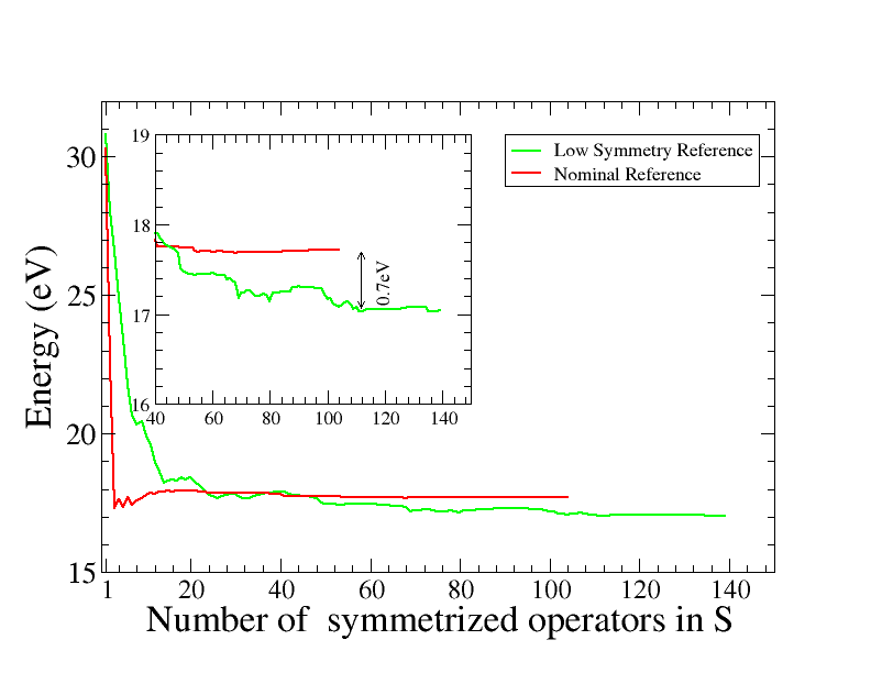
Figure 2: Convergence of the $CCM$ energies for a non-truncated Hilbert space ($U_{p}\simeq 5eV$). The nominal reference generates the first excited state while the lower symmetry reference state $\left|\bar{\Phi}_{0}\right>$ gives the ground state.

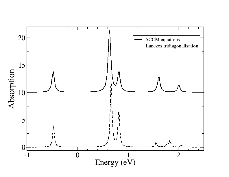
Figure 3: Spectra for the out-of-plane to in-plane probe $D_{cf}$ applied on the first excited eigenvalue, $U_{p}=10^{2}eV$ (truncated hilbert space)

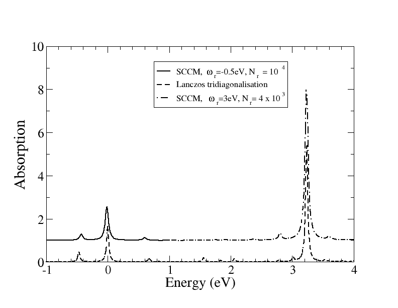
Figure 4: Spectra for the o charge transfer probe $D_{ch}$ applied on the first excited eigenvalue of the truncated problem ( $U_{p}=10^{2}eV$ )

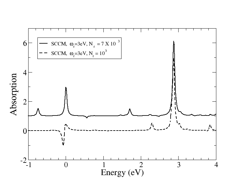
Figure 5: Spectra for the charge transfer probe $D_{ch}$ applied on the first excited eigenvalue of the non truncated problem ( $U_{p}=5eV$ ).

References

- [1] Hermann G. Kummel, A Biography of the Coupled Cluster Method, in Recent Progress in Many-body theories, Proceedings of the 11th International Conference Manchester, UK, 9 - 13 July 2001
- [2] Rodney J. Bartlett and Monika Musial, Rev. Mod. Phys. 79, 291–352 (2007)
- [3] R. F. Bishop and P. H. Y. Li, Phys. Rev. A 83, 042111 (2011)
- [4] F. Petit and M. Roger, Phys. Rev. B 49, 3453–3456 (1994)
- [5] Henrik Koch and Poul Jørgensen, J. Chem. Phys. 93, 3333 (1990)
- [6] Crawford, T. D. and Ruud, K. (2011), Coupled-Cluster Calculations of Vibrational Raman Optical Activity Spectra. ChemPhysChem, 12: 3442–3448
- [7] N. Govind et al., Chemical Physics Letters Volume 470, Issues 4–6, 5 March 2009, Pages 353–357
- [8] Sourav Pal, M. Dourga Prasad and Debashis Mukherjee Theoretica chimica Acta (1985) 68: 125-138
- [9] A. Mirone, S. S. Dhesi, and G. Van der Laan, Eur. Phys. J. B 53, 23 (2006).
- [10] J. Herrero-Martin, A. Mirone, J. Fernandez-Rodriguez et al. Phys. Rev. B 82, 075112 (2010)
- [11] Alessandro Mirone Hilbert++ Manual http://arxiv.org/abs/0706.4170