Agent-based Versus Macroscopic Modeling of Competition and Business Processes in Economics and Finance

Abstract

We present examples of agent-based and stochastic models of competition and business processes in economics and finance. We start from as simple as possible models, which have microscopic, agent-based, versions and macroscopic treatment in behavior. Microscopic and macroscopic versions of herding model proposed by Kirman and Bass new product diffusion are considered in this contribution as two basic ideas. Further we demonstrate that general herding behavior can be considered as a background of nonlinear stochastic model of financial fluctuations.

1 Introduction

Statistically reasonable models of social and economic systems, first of all stochastic and agent-based, are of great interest for a wide scientific community of interdisciplinary researchers dealing with diversity of complex systems [1, 2, 3, 4]. Computer modeling is one of the key aspects of modern science, be it physical or social or economic science, [5, 6]. In case of complex system modeling it serves as a technique in the quest for the understanding of the interrelation between microscopic interactions of individual agents and macroscopic, colective, dynamics of the whole complex system. Nevertheless, some general theories or methods that are well developed in the natural and physical sciences can be helpful in the development of consistent micro and macro modeling of complex systems [3, 4, 7, 8, 9].

As computer modeling is very prominent and important in modern science, we start this paper by discussing our online publishing and collaboration platform, see Section 3. The open-source applets made available online on the website “Physics of Risk”, see [10], allow to reproduce most of the results presented in this paper. This is very important as reproducibility of the results is one of the key demands in scientific society [5, 6].

From the Section 4 we start discussing various models applicable in economics and finance, which highlight the important correspondence between microscopic, agent-based, and macroscopic, stochastic, modeling. In the opening Section 4, we present Kirman’s agent-based model (see [11] for original paper) and derive its stochastic alternative, which was also done by Alfarano et al. in [12] using a more complex manner. In the Section 5 we show that modified, unidirectional, Kirman’s agent based model can be seen as microscopic alternative to the widely known Bass diffusion model [13]. Further, in Section 6, we apply the stochastic treatment of the Kirman’s model for financial markets and obtain stochastic model of absolute return similar to the CEV process [14] and earlier proposed model of $1/f$ noise [15, 16, 17]. In the Section 8 we show that Kirman’s model possesses multifractal features, which are seen as an important feature of many natural phenomena [18]. Section 9 closes presented discussion with some definitions and results regarding burst duration statistics generated by the class of nonlinear SDE and observable in the financial markets.

In the last section, Section 10, we sum up everything discussed in this paper and share some ideas on future developments of the discussed research.

2 Review of the related works

Current on-going financial economic crisis provoked many papers calling for a revolution of economical thought and emphasizing a need for a wider applications of statistical physics in the research of social complexity [3, 8, 9, 19, 20, 21, 22, 23, 24, 25]. Most of them pointing out that agent based models are very important if one wants to effectively understand what is going on in the complex social and economic systems and the physical intuition might provide the important bridging between the macroscopic and microscopic modeling. These ideas somewhat traceback to the thoughts put down by Waldrop and Axelrod in the 1990s (see [4, 7]).

In the recent decades there were many attempts to create an agent-based model for the financial markets, yet no model so far is realistic enough and tractable to be considered as an ideal model [26]. One of the best examples of realistic models is so-called Lux and Marchesi model [27], which is heavily based on the behavioral economics ideas mathematically put down as utility functions for the agents in the market, thus it is considered to be very reasonable and realistic [26]. Yet this model is too complex, namely it has many parameters and complex agent interaction mechanics, to be analytically tractable. Another example of a very complex agent-based model would be Bornholdt’s spin model [28, 29], which is based on a certain interpretation of the well-known Ising model (for the details on the original model see any handbook on statistical physics (ex., [30])).

Some might argue that agent-based models need not to be analytically tractable and in fact that agent-based models are best suited to model phenomena, which is too complex to be analytically described [31]. But the recent developments show that many groups attempt to build a bridge between microscopic and macroscopic models. Possibly one of the earliest attempts to do so started from not so realistic, nor tractable “El Farol bar problem” [32]. This simple model quickly became known as the Minority Game [33] and over few years received analytic treatment [34]. Another prominent simple agent-based model was created by Kirman [11], which gained broader attention only very recently [12, 35, 36, 37]. In [38] we have given this model and extended analytical treatment and have shown that this model coincides with some prominent macroscopic, namely stochastic, models of the financial markets (see Section 7 of this work for more details). Another interesting development was made by following the aforementioned Bornholdt’s spin model, which has recently received an analytical treatment via mean-field formalism [39].

Our work in the modeling of complex social and economic systems has begun from the applications of nonlinear stochastic differential equations (abbr. SDE) seeking reproduce statistics of financial market data. The proposed class of equations has power law statistics evidently very similar to the ones observed in the empirical data. As all of this work (for broad review see [16]) was done by relying on the macroscopic phenomenological reasoning, we are now motivated to find the microscopic reasoning for the proposed equations. The development of the macroscopic treatments for the well established agent-based models appears to be the most consistent approach, as the movement in the opposite direction seems to be very complex and ambiguitious task. Thus we decided that we should select the simple agent-based models, which would have an expected macroscopic description. In this contribution we present a few examples of the agent-based modeling, based on the Kirman’s model, in the business and finance while showing that the examples have useful and informative macroscopic treatments.

Kirman’s ant colony model [11] is an agent-based model used to explain the importance of herding inside the ant colonies and economic systems (see the later works by Kirman (ex. [40]) and other authors, which develop on this idea, [12, 35]). The analogy can be drawn as human crowd behavior is ideologically and statistically similar in many senses. On our website, [10], we have presented interactive realizations of the original Kirman’s agent-based model (see [41]), of its stochastic treatment by Alfarano et al. [12] (see [42]) and of its treatment in the financial market scenario done by our group [38] (see [43, 44]).

The diffusion of new products is one of the key problems in marketing research, and also one of the fields where we see that Kirman’s model might be applied. The Bass diffusion model is a very prominent model related to this problem. This model is formulated as an ordinary differential equation, which might be used to forecast the number of adopters of the new successful product or service [13]. There were suggestions that such basic macroscopic description in marketing research can be studied using the agent-based modeling as well [45]. Thus it is a great opportunity to explore the correspondence between the micro and macro descriptions looking for the conditions under which both approaches converge. The Bass Diffusion model is of great interest for us as representing very practical and widely accepted area of business modeling. Web based interactive models, presented on the site [46] serve as an additional research instrument available for very wide community. On our website we also provide an interactive applet for the Bass diffusion treatment in terms of the modified Kirman’s model [47] (for details on modification see Section 5 of this work).

Another interesting problem tackled in this work is related to the dynamics of the intermittent behavior. This kind of behavior is observed in many different complex systems ranging from the geology (ex., earthquakes [48]) and astronomy (ex., sunspots [49]) to the biology (ex., neuron activity [50]) and finance [51]. Great review of the universality of the bursty behavior is given by Karsai et al. [52] and Kleinberg [53]. In [52] the bursting behavior is considered as a point process with threshold mechanism. In this contribution we analyze the class of nonlinear SDE exhibiting power law statistics and bursting behavior, which was derived from the multiplicative point process [54, 55, 56] with applications for the modeling of trading activity in financial markets [57, 58]. This provides a very general, via hitting time formalism [14, 59, 60], approach to the modeling of bursty behavior of trading activity and absolute return in the financial markets [61].

3 Web platform

Our web site [10] was setup using WordPress webloging software [62]. The setup pays to be user-friendly, powerful and easily extensible web publishing platform, which with some effort can be adapted to the scientist’s needs. There is a wide choice of plugins, which enable convenient usage of equations (mostly using LaTeX). While during the setup we found that bibliography management plugins were lacking at the time.

To accommodate our needs for equations we have worked on improving WP-Latex plugin (available from [63]). Namely we have introduced a possibility to write equations in both inline and ordinary math modes. Implemented equation labeling, numbering and referencing. And finally fixed some noticeable problems with vertical placement of the inline mode equations.

Another important task was to implement bibliography management and citations. For this cause we have used the bibtexParse PHP code (available from [64]) to setup BiBTeX backend. From this point on we have written our own original PHP code to link between bibtexParse, our database and WordPress. By using this plugin we can now easily manage and present our own papers (ex. generate our own bibliographies), papers we have read (tag them with keywords, write our own comments and etc.) and also communicate with the visitors using numerous citations.

Interactive models themselves are independent from the publishing framework. Most of them were implemented using the Java applet technology. Some of the applets were created using multi-paradigm simulation software AnyLogic [65], while the others were programmed from scratch using Java programing language [66]. AnyLogic was used in the most of agent-based scenarios as it is a very convenient tool for agent-based modeling, while programing from scratch gave us more control over the applets behavior needed while doing stochastic modeling.

Either way by compiling appropriate files one obtains Java applets, which can be included in to the articles written using WordPress. This way articles become interactive - visitor can both theoretically familiarize himself with the model and test if the claims made in the post describing model were true. This happens in the same browser window, thus the transition between theory and modeling appears to be seamless. Due to the fact that models are implemented as Java applets all of the numerical evaluation occurs on client machine, while the visitor must have Java Runtime Environment installed, and server load stays minimal. The requirement for JRE might appear to be cumbersome, but the technology is somewhat popular and freely available from Oracle Corp.

One of the goals of developing these models on the web site was to provide theoretical background of Bass Diffusion model and discuss practical steps on how such computer simulations can be created even with limited IT knowledge and further applied for varying purposes (see [46]). Thus, we have targeted small and medium enterprises to encourage them to use modern computer simulation tools for business planning, sale forecasting and other purposes.

Consequently computer models and their corresponding descriptions published at the [46] provide a relatively easy starting point to get acquainted with computer simulation in business. The published content enables site visitors to familiarize themselves with these models interactively, running the applets directly in a browser window, changing the parameter values and observing results. This significantly increases accessibility and dissemination of these simulations.

Our web site also offers another level of reproducibility by including source code files inside the Java applet files. In this way any willing user may use modern archiver software (ex., 7Zip) to obtain the source code. After doing so one can analyze source code and more deeply understand the presented models and their implementations. This is a very important level of reproducibility in the modern scientific context [5, 6].

4 Extended macroscopic treatment of Kirman’s model

There is an interesting phenomenon concerning behavior of ant colony. It appears that if there are two identical food sources nearby, or two identical paths to the same food source (the experiment done by Pasteels and Deneubourg [67, 68]), ants exploit only one of them at a given time. Evidently the food source which will be used at a given time is not certain. It is so as switches between food sources occur, though the food sources, or paths, remain the same.

One could assume that those different food sources are different trading strategies or, if putting it simply, the actions available to traders. Thus, one could argue that speculative bubbles and crashes in the financial markets are of similar nature as the exploitation of the food sources in ant colonies - as quality of stock and quality of food in the ideal case can be assumed to be constant. Thus, model [11] was created using ideas obtained from the ecological experiments [67, 68] can be applied towards the financial market modeling.

Kirman, as an economist, actually developed this model as a general framework in context of economic modeling (see [11, 40] and his other works). Recently his framework was also used by other authors who are concerned with the financial market modeling (see [12, 35]). Thus basing ourselves on the main ideas of these authors and our previous results in stochastic modeling (see [16]) we introduce specific modifications of Kirman’s model providing a class of nonlinear stochastic differential equations [17] applicable for the financial variables.

Kirman’s one step transition probabilities might be expressed in the following form [11],

$$p(X\rightarrow X+1) = (N-X)\left(\sigma_{1}+hX\right)\Delta t,$$ (1)

$$p(X\rightarrow X-1) = X\left(\sigma_{2}+h[N-X]\right)\Delta t,$$ (2)

where $X$ is a number of agents exploiting the chosen trading strategy (the one used to describe system state), while $N$ is a total number of agents in the system (thus the other trading strategy is used by the $N-X$ agents). In the above the original Kirman’s approach was extended by introducing fixed event time scale $\Delta t$ by replacing the original models individual decision $\varepsilon_{i}\rightarrow\sigma_{i}\Delta t$ and herding $(1-\delta)\rightarrow h\Delta t$ parameters. Later we will need a more general assumption that parameters $\sigma$ and $h$ may depend on $X$ and $N$, but for now we omit it.

Note that the transition probabilities (1) and (2) describe a scenario where the interaction among agent groups depends on the overall number of agents in alternative state. Such a choice makes the transition rates non-extensive, the connectivity between agent groups increases with the number of agents $N$. The herding interactions have a global character. Opposite scenario - extensive one will be also used further in this paper.

The lack of memory of the agents is the crucial assumption to formalize the population dynamics as a Markov process. Furthermore to describe the aforementioned dynamics in a continuous time we will need to obtain the transition rates, transition probabilities per unit time, which for continuous $x=X/N$ may be expressed as

$$\pi^{+}(x) = (1-x)\left(\frac{\sigma_{1}}{N}+hx\right),$$ (3)

$$\pi^{-}(x) = x\left(\frac{\sigma_{2}}{N}+h[1-x]\right).$$ (4)

Here the large number of agents $N$ is assumed to ensure the continuity of variable $x$, which expresses the fraction of agents using the selected trading strategy, $X$. Relation between the discrete transition probabilities, (1) and (2), and continuous transition rates, (3) and (4), should be evident:

$$p(X\rightarrow X\pm 1)=N^{2}\pi^{\pm}(x)\Delta t.$$ (5)

One can compactly express the Master equation for the system state probability density function, $\omega(x,t)$, by using one step operators ${\bf E}$ and ${\bf E^{-1}}$ (see [69] for a details on this formalism) as

$$\partial_{t}\omega(x,t)= N^{2}\left\{({\bf E}-1)[\pi^{-}(x)\omega(x,t)]+({\bf E^{-1}}-1)[\pi^{+}(x)\omega(x,t)]\right\}.$$ (6)

By expanding ${\bf E}$ and ${\bf E^{-1}}$ using the Taylor expansion (up to the second term) we arrive at the approximation of the Master equation

$$\partial_{t}\omega(x,t)= -N\partial_{x}[\{\pi^{+}(x)-\pi^{-}(x)\}\omega(x,t)]+\frac{1}{2}\partial^{2}_{x}[\{\pi^{+}(x)+\pi^{-}(x)\}\omega(x,t)].$$ (7)

By introducing custom functions

$$A(x) = N\{\pi^{+}(x)-\pi^{-}(x)\}=\sigma_{1}(1-x)-\sigma_{2}x,$$ (8)

$$D(x) = \pi^{+}(x)+\pi^{-}(x)=2hx(1-x)+\frac{\sigma_{1}}{N}(1-x)+\frac{\sigma_{2}}{N}x,$$ (9)

one can make sure that the (6) is actually a Fokker-Planck equation:

$$\partial_{t}\omega(x,t)=-\partial_{x}[A(x)\omega(x,t)]+\frac{1}{2}\partial^{2}_{x}[D(x)\omega(x,t)].$$ (10)

Note that in the limit of large $N$ one can neglect individual behavior terms in the $D(x)$. The above Fokker-Planck equation was first derived in a slightly different manner in the [12].

It is known (for details see [59]) that the Fokker-Planck equation can be rewritten as Langevin equation, or in other words stochastic differential equation,

$$\mathrm{d}x = A(x)\mathrm{d}t+\sqrt{D(x)}\mathrm{d}W=[\sigma_{1}(1-x)-\sigma_{2}x]\mathrm{d}t+\sqrt{2hx(1-x)}\mathrm{d}W,$$ (11)

here $W$ stands for Wiener process. This step was also present in the [12].

In Fig. 1 we show that the statistical properties obtained from the agent-based model, defined by transition probabilities (1) and (2), match statistical properties of the solutions of (11). Thus the approximations done while deriving the Langevin equation for population fraction are valid. Interestingly enough we have obtained agreement with not so high number of agents - $N=100$.

(a)

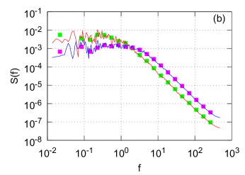
(b)

Figure 1: Agreement between statistical properties of population fraction, $x$, (a) probability density function and (b) power spectral density, obtained from stochastic (red and blue curves) and agent-based (green and magenta squares) models. Two qualitatively different model phases are shown: red curve and green squares correspond to herding dominant model phase ($\sigma_{1}=\sigma_{2}=0.2$, $h=5$), while blue curve and magenta squares correspond to individual behavior dominant model phase ($\sigma_{1}=\sigma_{2}=16$, $h=5$). Agent based model results obtained with $N=100$.

Note that the method used to derive Eq. (11) gives us an opportunity to consider parameters $\sigma_{1}$, $\sigma_{2}$, $h$ dependent on the variable $x$ and $N$. We will need this generalization in the further elaboration on various applications. From our point of view, the general form of SDE (11) derived from the very basic agent-based herding model provides a wide choice of opportunities in consistent micro and macro modeling of complex social systems.

5 Agent based model for the Bass Diffusion

The Bass Diffusion model is a tool to forecast the diffusion rate of new products or technologies [13]. Mathematically it is formulated as an ordinary differential equation

$$\partial_{t}X(t)=[N-X(t)]\left[\sigma+\frac{h}{N}X(t)\right],X(0)=0.$$ (12)

where $X(t)$ denotes the number of consumers at time $t$, $N$ can be seen as the market potential, being a starting number of the potential consumers (agents), $\sigma$ is the coefficient of innovation, the likelihood of an individual to adopt the product due to influence by the commercials or similar external sources, $h$ is the coefficient of imitation, a measure of likelihood that an individual will adopt the product due to influence by other people who already adopted the product. This nonlinear differential equation serves as a macroscopic description of new product adoption by customers widely used in business planning [45].

The agent-based approach to the same problem is related with modeling of product adoption by individual users, or agents. One can simulate diffusion process using computers, where individual decisions of adoption occur with specific adoption probability affected by the other individuals in the neighborhood. It is easy to show that Bass diffusion process is a unidirectional case of the Kirman’s herding model [11]. Indeed, let us define $x(t)$ in the same way as in previous section $x(t)=X(t)/N$, then the potential users will adopt the product at the same rate as in Kirman’s model agents switch from one state to another

$$\pi^{+}(x) = (1-x)\left(\frac{\sigma}{N}+\frac{h}{N}x\right).$$ (13)

$$\pi^{-}(x) = 0.$$ (14)

The form of (14) should be self explanatory - in case of the product diffusion agent should not be allow to withdraw from the consumer state, thus this transition probability should be forced to equal zero.

The mathematical form of (13) is not as evident, note that we have substituted $h$ with $\frac{h}{N}$ (compare with the original model transition probability (3)), and needs further discussion. Mathematically this substitution can be backed by the need for the stochastic term to become negligible in the limit of large $N$. In the modeled market terms this substitution means an introduction of the interaction locality - namely it is an assumption that each individual communicates only with his local partners (epidemic case).

One can compare the expression of the transition probability, (13), with the adoption probabilities of the Linear and GLM models of Bass Diffusion discussed in [70]. The match in expressions is clear in the small time step limit, $\Delta t\rightarrow 0$.

In case of the transition rates (13) and (14) the macroscopic description functions, namely drift, $A(x)$, and diffusion, $D(x)$, become

$$A(x) = N\pi^{+}(x)=(1-x)\left(\sigma+hx\right),$$ (15)

$$D(x) = \pi^{+}(x)=\frac{(1-x)}{N}\left(\sigma+hx\right).$$ (16)

In the large market potential limit, $N\gg 1$, $D(x)$ becomes negligible and thus one can consider the obtained equation to be equivalent to the Bass Diffusion ordinary differential equation (12) instead of the stochastic differential equation. This serves as a proof that Bass Diffusion is an unidirectional epidemic case of Kirman’s herding model. Though this simple relation looks straightforward, we derive it and confirm by numerical simulations in fairly original way.

In Figure 2 we demonstrate the correspondence between the Bass Diffusion model (macroscopic description) and unidirectional Kirman’s herding model (microscopic description). Both, agent-based and continuous, descriptions of the product adoption, $\Delta X$, converge while the market potential, $N$, or the selected observation time interval, $\tau$, become larger.

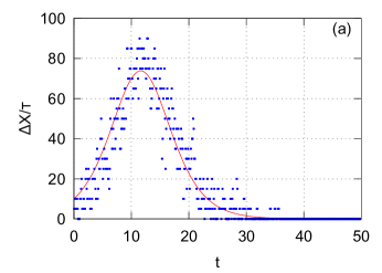
(a)

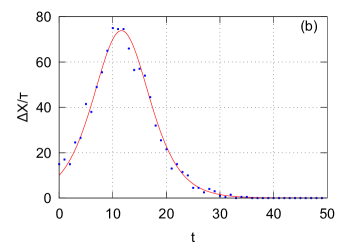
(b)

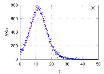
(c)

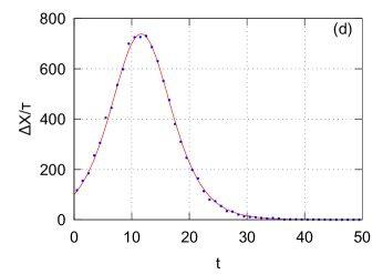
(d)

Figure 2: Comparison of the product adoption per observation interval, $\Delta X/\tau$ versus $t$, obtained from the macroscopic description by the Bass Diffusion model, (12), (red line) and the microscopic description using the unidirectional Kirman’s model, (13), (blue points). The models tend to converge when time window, $\tau$, or market potential, $N$, become larger: (a) $N=1000$, $\tau=0.1$; (b) $N=1000$, $\tau=1$; (c) $N=10000$, $\tau=0.1$; (d) $N=10000$, $\tau=1$. Other model parameters were the same for all subfigures and were as follows $\sigma=0.01$, $h=0.275$.

6 Nonlinear stochastic differential equation as a model of the financial markets

Earlier we have introduced a class of non-linear SDEs providing time series with power-law statistics, and most notably reproducing $1/f^{\beta}$ spectral density, [54, 55, 56]. The general form of the proposed class of Ito SDEs is

$$\mathrm{d}y=\left(\eta-\frac{\lambda}{2}\right)y^{2\eta-1}\mathrm{d}t_{s}+y^{\eta}\mathrm{d}W_{s},$$ (17)

here $y$ is the stochastic process exhibiting power-law statistics, $\eta$ is the power-law exponent of the multiplicative noise, while $\lambda$ defines the exponent of power-law probability density function (PDF), and $W$ is a Wiener process (the Brownian motion). Note that SDE (17) is defined in the scaled time, $t_{s}=\sigma_{t}^{2}t$, where $\sigma_{t}^{2}$ is the scaling parameter. Empirically we have determined that $\sigma_{t}^{2}=1/6\cdot 10^{-5}\mathrm{s}^{-1}$ is appropriate in terms of the return model proposed in [71].

From the SDE (17) follows that the stationary probability density function (PDF) of this stochastic process is power-law, $p_{0}(y)\sim y^{-\lambda}$, with the exponent $\lambda$ [59]. While in Refs. [72] and later more precisely in [17] it was shown that the time series obtained while solving SDE (17) have power-law spectral density

$$S(f)\sim\frac{1}{f^{\beta}},\qquad\beta=1+\frac{\lambda-3}{2(\eta-1)}.$$ (18)

Note that exponent of spectral density, $\beta$, is defined only for $\eta\neq 1$. In case of $\eta=1$ the SDE (17) becomes identical to the geometric Brownian motion.

Power law statistics of the signal $y$ obtained by solving SDE (17) and exponents $\lambda$, $\beta$ are defined for large $y$ values. Thus one has to introduce the diffusion restriction terms in the limit of small $y$ values when attempting to solve SDE (17) or applying it in a stochastic modeling. There is a wide choice of restriction mechanisms adjustable to the needs of real systems with negligible influence on the power law exponents. We have introduced a term of additive noise while attempting to model the absolute return [71]

$$\mathrm{d}y=\left(\eta-\frac{\lambda}{2}\right)(1+y^{2})^{\eta-1}y\mathrm{d}t_{s}+(1+y^{2})^{\frac{\eta}{2}}\mathrm{d}W_{s}.$$ (19)

In such case the stationary probability density function of the SDE (17) is a $q$-Gaussian (see [16, 71])

$$P_{\lambda}(y)=\frac{\Gamma(\lambda/2)}{\sqrt{\pi}\Gamma(\lambda/2-1/2)}\left(\frac{1}{1+y^{2}}\right)^{\frac{\lambda}{2}}.$$ (20)

While modeling the trading activity [58] we have used the exponential diffusion restriction for small values of variable $y\simeq y_{\mathrm{min}}$

$$\mathrm{d}y = \left[\eta-\frac{1}{2}\lambda+\frac{m}{2}\left(\frac{y_{\mathrm{min}}^{m}}{y^{m}}\right)\right]y^{2\eta-1}\mathrm{d}t+y^{\eta}\mathrm{d}W.$$ (21)

Equation (21) has a very general form, which includes the well known models applicable to financial markets such as the Cox-Ingersoll-Ross (CIR) process or the Constant Elasticity of Variance (CEV) process [14]

$$\mathrm{d}y=\mu y\mathrm{d}t+y^{\eta}\mathrm{d}W,$$ (22)

where $\mu=(\eta-1)y_{\mathrm{min}}^{2(\eta-1)}$, as a less general cases of the SDE (21).

The class of equations based on SDE (17) gives only a general idea how to model power-law statistics of trading activity and return in the financial markets. The problem is to determine the parameter set $\lambda$ and $\eta$ in a way giving the empirical values for the $\lambda$ and $\beta$. The task becomes even more complicated if one considers the more sophisticated behavior of the spectral density - power spectral densities have not one, but two power-law regions with different values of $\beta$. In the series of papers [71, 72, 58, 57] we have shown that trading activity and return can be modeled by a more sophisticated version of the SDE than (17) now including the two powers of the noise multiplicativity. In the case of return instead of Eq. (19) one should use

$$\mathrm{d}y = \left(\eta-\frac{\lambda}{2}\right)\frac{(1+y^{2})^{\eta-1}}{(\epsilon\sqrt{1+y^{2}}+1)^{2}}y\mathrm{d}t_{s}+\frac{(1+y^{2})^{\frac{\eta}{2}}}{\epsilon\sqrt{1+y^{2}}+1}\mathrm{d}W_{s},$$ (23)

here $\epsilon$ divides the area of diffusion into the two different noise multiplicativity regions to ensure the spectral density of $|y|$ with two power law exponents.

The proposed form of the SDE enables reproduction of the main statistical properties of the return observed in the financial markets. Similarly one can deal with a more sophisticated model for the trading activity [58]. This provides an approach to the financial markets with behavior dependent on the level of activity and exhibiting two stages: calm and excited. Equation (23) models the stochastic return $y$ with two power-law statistics, namely the probability density function and the power spectral density, reproducing the empirical power law exponents of the return in the financial markets.

7 Kirman’s model as a microscopic approach to the financial markets

The drawback of the stochastic models is a lack of direct insights into the microscopic nature of replicated dynamics. Bridging between microscopic and macroscopic approaches is needed for better grounding of stochastic modeling.

Top-down approach, namely starting from the stochastic modeling and moving towards the agent-based models, seems to be a very formidable task, as the macro-behavior of complex system can not be understood as a simple superposition of varying micro-behaviors. While in the case of sophisticated agent-based models [26] bottom-up approach provides too many opportunities. But there is selection of rather simple agent-based models (ex. [11]), whose stochastic treatment can be directly obtained from the microscopic description [12].

Here we consider an opportunity to generalize Kirman’s ant colony model [11] with the intention to modify its microscopic approach to the financial market modeling [12] reproducing the main stylized facts of this complex system. In the Section 4 we have already introduced Kirman’s ant colony model, proposed its generalization and derived stochastic model for the two state population dynamics.

As Kirman’s model considers the two available agent states one must define two types of agents acting inside the market in order to relate Kirman’s model to financial markets. Currently, the most common choice is assuming that agents can be either fundamentalists or noise traders [26].

Fundamentalists are assumed to have the fundamental knowledge about the market, which is assumed to be quantified by the so-called fundamental price, $P_{f}(t)$, of the traded stock. By having this knowledge they can make long term forecasts on a notion that infinitely long under-evaluation or over-evaluation of the stock is impossible - the market in some point in the future will have to set a fair price on the stock. Thus their excess demand, which is shaped by their long term expectations, is given by [12]

$$D_{f}(t)=N_{f}(t)\ln\frac{P_{f}(t)}{P(t)},$$ (24)

here $N_{f}(t)$ is a number of fundamentalists inside the market and $P(t)$ is a current market price. As long term investors fundamentalists assume that $P(t)$ will converge towards $P_{f}(t)$ at least in a long run. Therefore if $P_{f}(t)>P(t)$, fundamentalists will expect that $P(t)$ will grow in future and consequently they will buy the stock ($D_{f}(t)>0$). In the opposite case, $P_{f}(t)<P(t)$, they will expect decrease of $P(t)$ and for this reason they will sell the stock ($D_{f}(t)<0$).

The other group, the noise traders are investors who attempt estimate the stocks future price based on its recent movements. As there is a wide selection of technical trading strategies, which are used to analyze stocks price movements, one can simply assume that the average noise traders demand is based on their mood, $\xi(t)$, [12]

$$D_{c}(t)=r_{0}N_{c}(t)\xi(t),$$ (25)

here $D_{c}(t)$ is a total excess demand of noise trader group, $N_{c}(t)$ is a number of noise traders inside the market and $r_{0}$ can be seen as a relative noise trader impact factor.

Price and, later after a brief derivation, return can be introduced into the model by applying the Walrassian scenario. One can assume that trading in the market is cleared instantaneously to set a price, which would stabilize the market demand for a given moment. Thus the sum of all groups’ excess demands should equal zero:

$$D_{f}(t)+D_{c}(t) = N_{f}(t)\ln\frac{P_{f}(t)}{P(t)}+r_{0}N_{c}(t)\xi(t)=0,$$ (26)

$$P(t) = P_{f}(t)\exp\left[r_{0}\frac{N_{c}(t)}{N_{f}(t)}\xi(t)\right],$$ (27)

where without loosing generality one can assume that fundamental price remains constant, $P_{f}(t)=P_{f}$.

Consequently the return, which is defined as logarithmic change of price, in the selected time window $T$ is given by:

$$r(t) = \ln P(t)-\ln P(t-T)=r_{0}\left[\frac{x(t)}{1-x(t)}\xi(t)-\frac{x(t-T)}{1-x(t-T)}\xi(t-T)\right],$$ (28)

where we have set that $\frac{N_{c}(t)}{N}=x$ and $\frac{N_{f}(t)}{N}=1-x$ according to the notation introduced in Section 4. Alfarano et al. [12] simplified the above by assuming that $x(t)$ is significantly slower process than $\xi(t)$, obtaining adiabatic approximation of the return

$$r(t)=r_{0}\frac{x(t)}{1-x(t)}\zeta(t),$$ (29)

where $\zeta(t)=\xi(t)-\xi(t-T)$. If $\zeta(t)$ is modeled using spin-noise model, as in [12], then the middle term, $\frac{x(t)}{1-x(t)}$, can be seen as an absolute return.

Using Ito formula for variable substitution [59] in SDE (11) we obtain nonlinear SDE for the $y(t)=\frac{x(t)}{1-x(t)}$

$$\mathrm{d}y = (\sigma_{1}-y[\sigma_{2}-2h])(1+y)\mathrm{d}t+\sqrt{2hy}(1+y)\mathrm{d}W.$$ (30)

Agreement between the agent-based Kirman’s model applied towards financial markets using the ideas discussed above and the new stochastic model for $y$, (30), is demonstrated in Fig. 3.

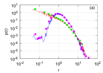
(a)

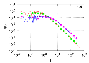
(b)

Figure 3: Agreement between statistical properties of $y$, (a) probability density function and (b) power spectral density, obtained from the stochastic (red and blue curves) and agent-based (green and magenta squares) models. Two qualitatively different model phases are shown: red curve and green squares correspond to herding dominant model phase ($\sigma_{1}=\sigma_{2}=0.2$, $h=5$), while blue curve and magenta squares correspond to individual behavior dominant model phase ($\sigma_{1}=\sigma_{2}=16$, $h=5$). Agent based model results obtained with $N=100$.

Note once again that the actual derivation, and thus, the final outcome, does not change even if $\sigma_{1}$, $\sigma_{2}$ or $h$ are the functions of either $x$ or $y$. Therefore, one can further study the possibilities of the obtained stochastic model, (30), by checking different scenarios of $\sigma_{1}$, $\sigma_{2}$ or $h$ being functions of either $x$ or $y$. Nevertheless, the most natural way is to introduce a custom function $\tau(y)$ to adjust the inter-event time according to the system state. From the financial market point of view this can be seen as introduction of variability of trading activity based on the return.

We have chosen the case when $h$ and $\sigma_{2}$ are functions of $y$, namely we make the substitutions, $\sigma_{2}\rightarrow\frac{\sigma_{2}}{\tau(y)}$ and $h\rightarrow\frac{h}{\tau(y)}$, in the Kirman’s model transition probabilities, (1) and (2), and stochastic model for $y$, (30). To further simplify the model we can introduce scaled time, $t_{s}=ht$, and make related model parameter transformations, $\varepsilon_{i}=\frac{\sigma_{i}}{h}$. By making these substitutions we arrive at

$$\mathrm{d}y = \left[\varepsilon_{1}+y\frac{2-\varepsilon_{2}}{\tau(y)}\right](1+y)\mathrm{d}t_{s}+\sqrt{\frac{2y}{\tau(y)}}(1+y)\mathrm{d}W_{s},$$ (31)

where $W_{s}$ is appropriately scaled Wiener process. Note that we left $\sigma_{1}$, and consequently $\varepsilon_{1}$, independent of $y$ on purpose as one could argue that individual behavior of fundamentalist trader should not depend on the observed returns as he is a long term investor uninterested in the momentary fluctuations of the market mood.

Note that absolute return, $y$, defined in Eqs. (30) and (31), serve as a measure of volatility in the financial markets. It is known that volatility has long-range memory and correlates with trading activity and has probability density function with power law tail [51]. We are particularly interested in the case of $\tau(y)=y^{-\alpha}$. This selection is defined by the fact that trading activity has positive correlation with volatility and the class of SDE (17) is invariant regarding power-law variable transformation, see [56]. In such case the obtained stochastic differential equation, Eq. (31), in the limit of $y\gg 1$ is very similar to the stochastic models discussed in the Section 6.

In the aforementioned limit of $y$, $y\gg 1$, we can consider only the highest powers in Eq. (31). In such case Eq. (31) is reduce to the

$$\mathrm{d}y=(2-\varepsilon_{2})y^{2+\alpha}\mathrm{d}t_{s}+\sqrt{2y^{3+\alpha}}\mathrm{d}W_{s}.$$ (32)

The direct comparison of Eqs. (17) and (32) yields:

$$\eta=\frac{3+\alpha}{2},\quad\lambda=\varepsilon_{2}+\alpha+1.$$ (33)

Consequently we expect that the stochastic process $y$ defined by Eq. (32) will have the power law stationary probability density function,

$$p(y)\sim y^{-\varepsilon_{2}-\alpha-1},$$ (34)

and also a power law spectral density,

$$S(f)\sim\frac{1}{f^{\beta}},\quad\beta=1+\frac{\varepsilon_{2}+\alpha-2}{1+\alpha},$$ (35)

where we have used the relation between model parameters, Eq. (33).

While if we linearize drift function of Eq. (30) with the respect to the absolute return, $y$, namely set $\varepsilon_{2}=2$, we would obtain a stochastic differential equation (once again in the limit $y\gg 1$)

$$\mathrm{d}y=\varepsilon_{1}y\mathrm{d}t_{s}+\sqrt{2y^{3+\alpha}}\mathrm{d}W_{s}.$$ (36)

similar to the generalized CEV process [14, 73], which was considered in [73],

$$\mathrm{d}y=ay\mathrm{d}t+by^{\eta}\mathrm{d}W.$$ (37)

In [56] the latter was noted to be a special case of Eq. (21) with exponential restriction of diffusion applied. The comparison with this special case is important on its own as this equation generalizes some stochastic models used in risk management. Theoretical prediction of PDF and spectral density for $y$ defined by Eq. (36), is given by [73]

$$p(y)\sim y^{-3-\alpha},$$ (38)

$$S(f)\sim\frac{1}{f^{\beta}},\quad\beta=1+\frac{\alpha}{1+\alpha},$$ (39)

where we have used the previously obtained relation between model parameters, Eq. (33).

In the Figure 4 we show that the theoretical predictions discussed in this section are valid and that they enable the reproduction of different spectral densities and probability density functions.

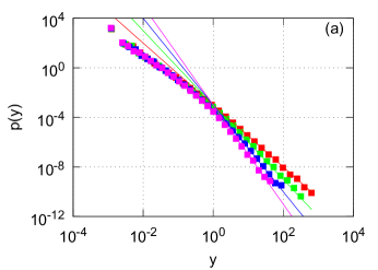
(a)

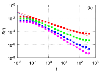
(b)

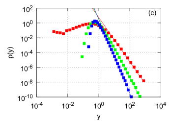
(c)

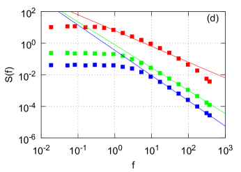
(d)

Figure 4: Statistical properties, (a) and (c) - probability density function, (b) and (d) - spectral density, of the time series obtained by solving Eq. (31) (colored squares). Fits are provided by the theoretical predictions made in this section, (a) and (b) are fitted by using (34) and (35), (c) and (d) are fitted by using (38) and (39), (curves of corresponding colors). Model parameters for the (a) and (b) were set as follows: $\alpha=1$, $\varepsilon_{1}=0$, $\varepsilon_{2}=0.5$ (red squares), $1$ (green squares), $1.5$ (blue squares) and $2$ (magenta squares). Model parameters for the (c) and (d) were set as follows: $\varepsilon_{1}=\varepsilon_{2}=2$, $\alpha=0$ (red squares), $1$ (green squares) and $2$ (blue squares).

Note that while the stochastic model based on herding behavior of agents appears to be too crude to reproduce statistical properties of financial markets in such details as the stochastic model driven by the Eq. (23), which is heavily based on the empirical research, it contains very important long range power law statistics of the absolute return. Obtained equations are very similar to some general stochastic models of the financial markets [17, 73] and thus, in future development might be able to serve as a microscopic justification for them and maybe for the more sophisticated model driven by the Eq. (23).

It is possible to extend agent-based model by introducing additional agent groups or splitting old ones. Let us assume that chartist agents may disagree in their expectations and thus divide into pessimists and optimists. Therefore it is natural to introduce three agent groups (see Fig. 5) interacting among themselves.

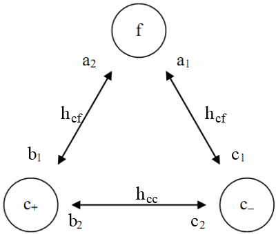
(a)

Figure 5: The general case of the three groups of interacting agents: $f$ - fundamentalists, $c_{+}$ - chartists optimists, $c_{-}$ - chartists pessimists. $h_{ij}$ are herding terms, while $a_{i}$, $b_{i}$ and $c_{i}$ stand for individual transitions in the direction of the arrow.

Our first attempts in this direction proves that in case of the three agent groups (as shown in Fig. 5), when the herding parameter $h_{cc}\gg h_{cf}$, might confirm the expectation of a more complex behavior exhibiting fractured power spectral density of absolute return. More detailed study of such approach in comparison with macroscopic modeling by SDE (23) is ongoing.

8 Multifractal behavior of return series

In the last few decades it was noted that many natural phenomena have very complex intrinsic structure, which has a very specific scaling properties. This notion was generalized as fractal framework [74]. Later it was also noted that the scaling properties of some processes exhibit even more complex scaling behavior - namely they appeared to have features of the multiple fractals. Few examples of such phenomena include geoelectrical processes [75], human heartbeat [76] and gait [77]. The financial market time series apparently are also of the multifractal nature [78, 79, 80].

There are few established methods to detect multifractal time series and two very prominent methods. One of them is generalized height-height correlation function method (GHHCF) and multifractal detrended analysis method (MF-DFA). In our previous approaches [81, 38] we have used the GHHCF method, so let us in this contribution to rely on the MF-DFA method.

To start with the multifractal analysis of the time series, $y_{k}$, we have to obtain the profile of the time series, $Y_{k}$:

$$Y_{k}=\sum_{j=1}^{k}(y_{k}-\langle y\rangle).$$ (40)

Next we have divide the $Y_{k}$ series into equally sized and non overlapping segments. Thus if our segments are of the size $s$, then we will have $N_{s}=\mathrm{int}(N/s)$ segments (here $N$ is the length the series, while $\mathrm{int}(\dots)$ is a function which takes an integer part of the argument). For the most of the segment sizes some of the data will be lost, in order to account for it one might want to take another set of segments, but now splitting from the end of the series.

Further, one has to determine the trends in the obtained segments. Generally this can be done using varying polynomial fits, but linear fits in the most cases are more than enough. After the trends, $\bar{Y}$, are known one has to evaluate how well the trend fits the actual series:

$$F^{2}_{\nu}(s) = \frac{1}{s}\sum_{i=1}^{s}\left[Y_{(\nu-1)s+i}-{\bar{Y}}_{\nu}(i)\right]^{2},$$ (41)

$$F^{2}_{\nu}(s) = \frac{1}{s}\sum_{i=1}^{s}\left[y_{N-(\nu-N_{s})s+i}-{\bar{y}}_{\nu}(i)\right]^{2}.$$ (42)

The Eq. (41) holds for segments $\nu=1,\ldots,N_{s}$, while the Eq. (42) should applied towards segments $\nu=N_{s}+1,\ldots,2N_{s}$. Finally one has to average over all segments using

$$F_{q}(s)=\left\{\frac{1}{2N_{s}}\sum_{\nu=1}^{2N_{s}}\left[F^{2}_{\nu}(s)\right]^{\frac{q}{2}}\right\}^{\frac{1}{q}},$$ (43)

here $q$ stands for generalized coefficient, which is the one enabling us to recover multifractal features – it is also the only difference from the original detrended fluctuation analysis (DFA) method [18]. Note that in case of $q=2$ the $F_{q}(s)$ is the same as the one in the original DFA method.

All that is left is to determine is the power law trend, $h(q)$, of the $F_{q}(s)$. These trends, $h(q)$, are also frequently named the generalized Hurst exponents. If the Hurst exponents are different for different $q$, which can be any real number, then the signal can be seen as multifractal. In the opposite case or if the variation is negligible, time series can be assumed as monofractal. For more details on the MF-DFA method see [18].

In Figure 6 we show that the stochastic differential equations obtained for the modeling of financial markets and derived from the Kirman’s agent-based model have broad multifractal spectra. The curves capture a region of the Brownian motion, $h(q)\approx 1.5$, and a region of long range memory, $h(q)\approx 1$. Note that in case of $\alpha=1$ and $\alpha=2$ (green and blue curves) $h(2)=1$, which can be seen as a proof that the obtained time series posses the long term correlated (have so-called long range memory) behavior, while for $\alpha=0$ interim behavior between the Brownian motion and long range memory is observed, $1<h(2)<1.5$.

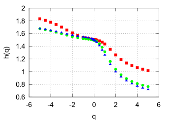
(a)

Figure 6: The broad spectra of Hurst exponents, $h(q)$, obtained from time series obtained by solving (31). The model parameters were set as follows: $\varepsilon_{1}=1$, $\varepsilon_{2}=2-\alpha$, $\alpha=0$ (red squares), $1$ (green circles) and $2$ (blue triangles).

9 Statistics of bursts generated by nonlinear SDE

In the Section 7 we have shown that the herding model of return in the financial markets leads to the class of stochastic differential equations, whose general form is given by SDE (17). This class of stochastic differential equations reproduces power law statistics, namely the probability density function and the spectral density, of return and trading activity in the financial markets. The burst statistics of the financial markets are also very important for the risk management and would serve as an additional criteria to determine the model consistency. In this section we provide some initial results of burst statistics generated by the SDE (17).

We define a burst as a part of the time series lying above the certain threshold, $h_{I}$. In Figure 7 we present an example burst of the simple bursty time series, $I(t)$. Evidently a burst as itself can be described by its duration, $T=t_{2}-t_{1}$, maximum value, $I_{max}$, and burst size, which we define as an area above the selected threshold yet bellow time series curve (highlighted by x pattern in the Fig. 7), $S$.

(a)

Figure 7: Time series exhibiting bursty behavior, $I(t)$. Here $h_{I}$ is the threshold value, above which bursts are detected, $t_{i}$ is the three visible threshold passage events, $I_{max}$ is the highlighted burst’s peak value. Burst duration we define as: $T=t_{2}-t_{1}$.

There is a well established passage, or alternatively hitting, time framework, which is frequently used to tackle practical problems in both mathematical finance [14] and physics [59, 60]. One can also apply this framework to understand the burst durations, $T$. Interestingly enough we can consider the first hitting time of the stochastic process starting infinitesimally near the hitting threshold as the burst duration itself, $T$.

Brownian motion, geometric Brownian motion and Bessel process are highly applicable models (for examples of the application in the mathematical finance, see [14]) for which hitting times statistics are known. The Bessel process,

$$\mathrm{d}R=\frac{N-1}{2}\frac{\mathrm{d}t_{s}}{R}+\mathrm{d}W_{s},$$ (44)

is one of the most interesting as some prominent mathematical finance models can be transformed to a similar form. In order to simplify further handling of the Bessel process it is convenient to introduce $\nu=\frac{N}{2}-1$, which is known as the index of the Bessel process. While $N$ is also frequently retained and mentioned as it bears an actual physical meaning - the Bessel process is an Euclidean norm, length of the vector, of $N$-dimensional Brownian motion, which starts at the origin. Note that for $N>1$, or alternatively $\nu>-0.5$, $R$ tends to diverge towards infinity.

In our case the Bessel process is of high interest as by using the Lamberti transform defined as

$$\ell:y\mapsto z(y)=\frac{1}{(\eta-1)y^{\eta-1}},$$ (45)

we can reduce a general class of SDE (17) to the Bessel process,

$$\mathrm{d}z=\left(\nu+\frac{1}{2}\right)\frac{\mathrm{d}t_{s}}{z}+\mathrm{d}W_{s},$$ (46)

with index $\nu=\frac{\lambda-2\eta+1}{2(\eta-1)}$. The corresponding dimension of the Brownian motion is given by $N=2(\nu+1)=\frac{\lambda-1}{\eta-1}$.

Let us assume that a burst starts at time $t_{0}$, with $y_{0}=y(t_{0})$ slightly exceeding the selected threshold, $h_{y}$. By definition the burst lasts until $y(t)$ crosses $h_{y}$ once again, but now from the above. Equivalently, in the terms of Bessel process the burst lasts until at a certain time, $t$, the $z$ process crosses the boundary $h_{z}=\ell(h_{y})$ from the below, while the starting position, $z_{0}=z(t_{0})$, which in the terms of Bessel process is below the threshold, $z_{0}=\ell(y_{0})<h_{z}$.

Consequently by choosing $z_{0}$ arbitrarily close yet below $h_{z}$, we can obtain an estimate for the burst duration, $T$, in terms of the hitting times of the Bessel process, $\tau^{(\nu)}_{z_{0},h_{z}}$,

$$T = \tau^{(\nu)}_{z_{0},h_{z}}=\inf_{t>t_{0}}\Big{\{}t,\>z(t)\geq h_{z}\Big{\}},0<h_{z}-z_{0}<\epsilon,$$ (47)

where $\epsilon$ is an arbitrary small positive constant. As given in [82], the following holds for $0<z_{0}<h_{z}$

$$\rho^{(\nu)}_{z_{0},h_{z}}(t) = \frac{h_{z}^{\nu-2}}{z_{0}^{\nu}}\sum_{k=1}^{\infty}\left[\frac{j_{\nu,k}J_{\nu}\left(\frac{z_{0}}{h_{z}}j_{\nu,k}\right)}{J_{\nu+1}(j_{\nu,k})}\exp\left(-\frac{j_{\nu,k}^{2}}{2h_{z}^{2}}t\right)\right],$$ (48)

where $\rho_{z_{0},h_{z}}^{(\nu)}(t)$ is a probability density function of the hitting times at level $h_{z}$ of Bessel process with index $\nu$ starting from $z_{0}$, $J_{\nu}$ is a Bessel function of the first kind of the order $\nu$, while $j_{\nu,k}$ is a $k$-th zero of $J_{\nu}$.

We have to replace $\rho^{(\nu)}_{z_{0},h_{z}}(t)$ by density function regarding $h_{z}$ to avoid the self-evident convergence of $\rho^{(\nu)}_{z_{0},h_{z}}(t)$ (for $t>0$) to zero, when $z_{0}\rightarrow h_{z}$. This is achieved introducing the probability density function $p_{h_{z}}^{(\nu)}(t)$ as a probability density function of the burst duration

$$p_{h_{z}}^{(\nu)}(t)=\lim_{z_{0}\rightarrow h_{z}}\frac{\rho^{(\nu)}_{z_{0},h_{z}}(t)}{h_{z}-z_{0}},$$ (49)

where we have selected the threshold at level $h_{z}$ and $\nu$ is the original model parameter. To evaluate this limit we have to expand $J_{\nu}\left(\frac{z_{0}}{h_{z}}j_{\nu,k}\right)$ near $\frac{z_{0}}{h_{z}}=1$:

$$J_{\nu}\left(\frac{z_{0}}{h_{z}}j_{\nu,k}\right) \approx J_{\nu}(j_{\nu,k})-\left(1-\frac{z_{0}}{h_{z}}\right)\left[\nu J_{\nu}(j_{\nu,k})-j_{\nu,k}J_{1+\nu}(j_{\nu,k})\right]=(1-\frac{z_{0}}{h_{z}})j_{\nu,k}J_{1+\nu}(j_{\nu,k}).$$ (50)

By using this expansion we can rewrite (49) as:

$$p_{h_{z}}^{(\nu)}(t)\approx C_{1}\sum_{k=1}^{\infty}j_{\nu,k}^{2}\exp\left(-\frac{j_{\nu,k}^{2}}{2h_{z}^{2}}t\right),$$ (51)

here $C_{1}$ is a normalization constant. By taking a note that $j_{\nu,k}$ are almost equally spaced, we can replace the sum by integration

$$p_{h_{z}}^{(\nu)}(t)\approx C_{2}\int_{j_{\nu,1}}^{\infty}x^{2}\exp\left(-\frac{x^{2}t}{2h_{z}^{2}}\right)\mathrm{d}x=C_{2}\left[\frac{h_{z}^{2}j_{\nu,1}\exp\left(-\frac{j_{\nu,1}^{2}t}{2h_{z}^{2}}\right)}{t}+\sqrt{\frac{\pi}{2}}\frac{h_{z}^{3}\mathrm{erfc}\left(\frac{j_{\nu,1}\sqrt{t}}{\sqrt{2}h_{z}}\right)}{t^{3/2}}\right].$$ (52)

From the expression above follows that the probability density of the burst durations in the time series obtained by solving SDE (17) can be approximated by a power law with exponential cut-off. Or mathematically

$$p_{h_{z}}^{(\nu)}(t)\sim t^{-3/2},\quad\textrm{for}\quad t\ll\frac{2h_{z}^{2}}{j_{\nu,1}^{2}},$$ (53)

$$p_{h_{z}}^{(\nu)}(t)\sim\frac{\exp\left(-\frac{j_{\nu,1}^{2}t}{2h_{z}^{2}}\right)}{t},\quad\textrm{for}\quad t\gg\frac{2h_{z}^{2}}{j_{\nu,1}^{2}}$$ (54)

This result is in agreement with a general property of one dimensional diffusion processes presented in [60], namely that the asymptotic behavior of first hitting times is a power law $t^{-3/2}$ irrespectively of the nature of stochastic one dimensional process or the actual mathematical expressions of the Langevin or the Fokker-Plank equations. The exponential cutoff for longer burst durations can be explained by the direction preference of the Bessel processes (note the positive drift term in case of $N>1$, or alternatively $\nu>-0.5$). The actual empirical data, as shown in Fig. 8 (b), also has the predicted asymptotic behavior, though the inconsistence in fitting is clearly higher than for the model’s probability density Fig. 8 (a).

(a)

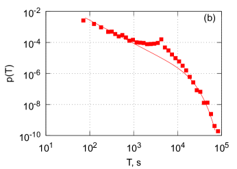
(b)

Figure 8: Numerical (a) and empirical (b) PDF of burst durations, $h_{y}=2$. In both subfigures numerical and empirical data is represented by filled shapes, while fits, (52), are represented by gray curves. Model, (17), parameters were set as follows: $\sigma_{t}^{2}=1/6\cdot 10^{-5}\mathrm{s}^{-1}$ (in all three cases), $\lambda=4$ (in all three cases), $\eta=2.5$ (red squares, $\nu=0$), $\eta=2$ (green circles, $\nu=0.5$) and $\eta=1.5$ (blue triangles, $\nu=2$). Empirical data fitted by assuming that $\nu=-0.2$.

Our empirical data set includes all trades made on NYSE, which were made from January, 2005 to March, 2007 and involved 24 different stocks, ABT, ADM, BMY, C, CVX, DOW, FNM, GE, GM, HD, IBM, JNJ, JPM, KO, LLY, MMM, MO, MOT, MRK, SLE, PFE, T, WMT, XOM. We have used one hour window moving average filter on empirical one minute return series. As we consider the model to be universal, i.e., applicable towards the modeling of varying financial markets and stocks, we can consider each stocks’ time series as a separate realization of the same stochastic process. Time series are first normalized and later averaged over the whole set. We back this approach by recalling that in [16] we have shown that the more sophisticated versions of (23) may be well used to model absolute return of different stocks from NYSE and Vilnius Stock Exchange.

There are numerous reasons for the observed inconsistence in fitting of empirical data Fig. 8 (b). Firstly, we were unable to remove intra-day pattern from the time series. But the main reason is that the simple stochastic model, driven by (17), is unable to reproduce the full complexity of empirically observed spectral density. In order to reproduce the correct, fractured, shape of the spectral density one must use double stochastic model, driven by a more sophisticated version SDE (23), [16]. Nevertheless, derived equations for the burst duration distribution (51) and (52) of the general process (17) are in agreement with empirical time series of return. This provides one more argument for the further development of stochastic models based on herding behavior of agents and nonlinear SDE (17).

10 Conclusions and future work

Reasoning of stochastic models of complex systems by the microscopic interactions of agents is still a challenge for researchers. Only very general models such as Kirman’s herding model in ant colony or Bass diffusion model for new product adoption have well established agent-based versions and can be described by stochastic or ordinary differential equations. There are many different attempts of microscopic modeling in more sophisticated systems, such as financial markets or other social systems, intended to reproduce the same empirically defined properties. The ambiguity of microscopic description in complex systems is an objective obstacle for quantitative modeling. Simple enough agent-based models with established or expected corresponding macroscopic description are indispensable in modeling of more sophisticated systems. In this contribution we discussed various extensions and applications of Kirman’s herding model.

First of all, we modify Kirman’s model introducing interevent time $\tau(y)$ or trading activity $1/\tau(y)$ as functions of driving return $y$. This produces the feedback from macroscopic variables on the rate of microscopic processes and strong nonlinearity in stochastic differential equations responsible for the long range power-law statics of financial variables. We do expect further development of this approach introducing the mood of chartists as independent agent-based process.

Nonlinear SDEs derived from the agent herding model generate multifractal time series. This gives more confidence in the modeling of multifractal series observed in financial markets. We derive PDF of burst duration for the basic form of nonlinear SDE (17). This is in agreement with empirical time series of return. Further investigation of burst statistics in financial markets in comparison with analytical results from nonlinear SDE is ongoing. This would serve as an independent method to adjust model parameters to the empirical data.

One more outcome of Kirman’s herding behavior of agents is one direction process - Bass diffusion. This simple example of correspondence between very well established microscopic and macroscopic modeling becomes valuable for further description of diffusion in social systems. Models presented on the interactive web site [10] have to facilitate further extensive use of computer modeling in economics, business and education.

References

- [1] V. Daniunas, V. Gontis, and A. Kononovicius, “Agent-based versus macroscopic modeling of competition and business processes in economics,” in ICCGI 2011, The Sixth International Multi-Conference on Computing in the Global Information Technology, Luxembourg, 2011, pp. 84–88.
- [2] D. Helbing, Managing Complexity: Insights, Concepts, Applications. Springer, 2008.
- [3] L. Pietronero, “Complexity ideas from condensed matter and statistical physics,” Europhysics news, vol. 39, pp. 26–29, 2008.
- [4] M. Waldrop, Complexity: The emerging order at the edge of order and chaos. New York: Simon and Schuster, 1992.
- [5] D. C. Ince, L. Hatton, and J. Graham-Cumming, “The case for open computer programs,” Nature, vol. 482, pp. 485–488, 2012.
- [6] K. Niemeyer, “If you want reproducible science, the software needs to be open source,” Nature Editorial, 2012. [Online]. Available: http://arstechnica.com/science/2012/02/science-code-should-be-open-source-according-to-editorial/ [Accessed: 2012-06-14]
- [7] R. Axelrod, “Advancing the art of simulation in the social sciences,” Complexity, vol. 3, no. 2, pp. 16–32, 1998.
- [8] D. Helbing, “Pluralistic modeling of complex systems,” Science and Culture, vol. 76, no. 2, p. 315, 2010.
- [9] J. H. Johnson, “The future of the social sciences and humanities in the science of complex systems,” The European Journal of Social Science Research, vol. 23, no. 2, pp. 115–134, 2010.
- [10] V. Gontis, A. Kononovicius, and V. Daniunas, “Physics of risk.” [Online]. Available: http://mokslasplius.lt/rizikos-fizika/en [Accessed: 2012-06-11]
- [11] A. P. Kirman, “Ants, rationality and recruitment,” Quarterly Journal of Economics, vol. 108, pp. 137–156, 1993.
- [12] S. Alfarano, T. Lux, and F. Wagner, “Estimation of agent-based models: The case of an asymmetric herding model,” Computational Economics, vol. 26, no. 1, pp. 19–49, 2005.
- [13] F. M. Bass, “A new product growth model for consumer durables,” Management Science, vol. 15, pp. 215–227, 1969.
- [14] M. Jeanblanc, M. Yor, and M. Chesney, Mathematical Methods for Financial Markets. Berlin: Springer, 2009.
- [15] B. Kaulakys and M. Alaburda, “Modeling scaled processes and noise using non-linear stochastic differential equations,” Journal of Statistical Mechanics, p. P02051, 2009.
- [16] V. Gontis, J. Ruseckas, and A. Kononovicius, “A non-linear stochastic model of return in financial markets,” in Stochastic Control, C. Myers, Ed. InTech, 2010.
- [17] J. Ruseckas and B. Kaulakys, “1/f noise from nonlinear stochastic differential equations,” Physical Review E, vol. 81, p. 031105, 2010.
- [18] J. W. Kantelhardt, S. A. Zschiegner, E. Koscielny-Bunde, S. Havlin, A. Bunde, and H. E. Stanley, “Multifractal detrended fluctuation analysis of nonstationary time series,” Physica A, vol. 316, pp. 87–114, 2002.
- [19] J. P. Bouchaud, “Economics need a scientific revolution,” Nature, vol. 455, p. 1181, 2008.
- [20] ——, “The (unfortunate) complexity of the economy,” Physics World, pp. 28–32, April 2009.
- [21] ——, “The Bachelier legacy: Why and how do asset prices move?” Siena, Italy, 2010, talk given at International School on Multidisciplinary Approaches to Economic and Social Complex Systems.
- [22] J. D. Farmer and D. Foley, “The economy needs agent-based modelling,” Nature, vol. 460, pp. 685–685, 2009.
- [23] T. Lux and F. Westerhoff, “Economic crysis,” Nature Physics, vol. 5, pp. 2–3, 2009.
- [24] M. E. J. Newman, “Complex systems: A survey,” American Journal of Physics, vol. 79, pp. 800–810, 2011.
- [25] C. Schinckus, “Econophysics and economics: Sister disciplines?” American Journal of Physics, vol. 78, no. 4, pp. 325–327, 2010.
- [26] M. Cristelli, L. Pietronero, and A. Zaccaria, “Critical overview of agent-based models for economics,” in Proceedings of the School of Physics ”E. Fermi”, course CLXXVI, Varenna, 2010.
- [27] T. Lux and M. Marchesi, “Scaling and criticality in a stochastic multi-agent model of a financial market,” Nature, vol. 397, pp. 498–500, 1999.
- [28] S. Bornholdt, “Expectation bubbles in a spin model of markets: Intermittency from frustration across scales,” International Journal of Modern Physics C, vol. 12, no. 5, pp. 667–674, 2001.
- [29] T. Kaizoji, S. Bornholdt, and Y. Fujiwara, “Dynamics of price and trading volume in a spin model of stock markets with heterogeneous agents,” Physica A, vol. 316, pp. 441–452, 2002.
- [30] J. P. Sethna, Statistical Mechanics: Entropy, Order Parameters and Complexity. Oxford: Clarendon Press, 2009.
- [31] E. Bonabeau, “Agent-based modeling: Methods and techniques for simulating human systems,” Proceedings of National Academy of Science USA, vol. 99, no. Suppl 3, pp. 7280–7287, 2002.
- [32] W. B. Arthur, “Inductive reasoning and bounded rationality,” American Economic Review, vol. 84, pp. 406–411, 1994.
- [33] D. Challet and Y.-C. Zhang, “Emergence of cooperation and organization in an evolutionary game,” Physica A, vol. 246, pp. 407–418, 1997.
- [34] D. Challet, M. Marsili, and R. Zecchina, “Statistical mechanics of systems with heterogeneous agents: Minority games,” Physical Review Lettets, vol. 84, pp. 1824–1827, 2000.
- [35] S. Alfarano, T. Lux, and F. Wagner, “Time variation of higher moments in a financial market with heterogeneous agents: An analytical approach,” Journal of Economic Dynamics and Control, vol. 32, pp. 101–136, 2008.
- [36] V. Alfi, M. Cristelli, L. Pietronero, and A. Zaccaria, “Minimal agent based model for financial markets i: Origin and self-organization of stylized facts,” European Physics Journal B, vol. 67, no. 3, pp. 385–397, 2009.
- [37] ——, “Minimal agent based model for financial markets ii: Statistical properties of the linear and multiplicative dynamics,” European Physics Journal B, vol. 67, no. 3, pp. 399–417, 2009.
- [38] A. Kononovicius and V. Gontis, “Agent based reasoning for the non-linear stochastic models of long-range memory,” Physica A, vol. 391, no. 4, pp. 1309–1314, 2012.
- [39] S. M. Krause, P. Bottcher, and S. Bornholdt, “Mean-field-like behavior of the generalized voter-model-class kinetic ising model,” Physical Review E, vol. 85, p. 031126, 2012.
- [40] A. Kirman and G. Teyssiere, “Microeconomic models for long memory in the volatility of financial time series,” Studies in Nonlinear Dynamics and Econometrics, vol. 5, no. 4, pp. 281–302, 2002.
- [41] A. Kononovicius and V. Gontis, “Kirman’s ant colony model.” [Online]. Available: http://mokslasplius.lt/rizikos-fizika/en/kirman-ants [Accessed: 2012-06-11]
- [42] ——, “Stochastic ant colony model.” [Online]. Available: http://mokslasplius.lt/rizikos-fizika/en/stochastic-ant-colony-model [Accessed: 2012-06-11]
- [43] ——, “Agent based herding model of financial markets.” [Online]. Available: http://mokslasplius.lt/rizikos-fizika/en/agent-based-herding-model-financial-markets [Accessed: 2012-06-15]
- [44] ——, “Multifractality of time series.” [Online]. Available: http://mokslasplius.lt/rizikos-fizika/en/multifractality-time-series [Accessed: 2012-06-15]
- [45] V. Mahajan, E. Muller, and F. M. Bass, “New-product diffusion models,” in Handbooks in Operations Research and Management Science, J. Eliashberg and G. L. Lilien, Eds. Amsterdam: North Holland, 1993, vol. 5, pp. 349–408.
- [46] V. Daniunas, “Verslo modeliai.” [Online]. Available: http://mokslasplius.lt/rizikos-fizika/category/business [Accessed: 2012-06-11]
- [47] A. Kononovicius and V. Gontis, “Unidirectional kirman’s model.” [Online]. Available: http://mokslasplius.lt/rizikos-fizika/en/unidirectional-kirman-model [Accessed: 2012-06-11]
- [48] A. Corral, “Long-term clustering, scaling, and universality in the temporal occurrence of earthquakes,” Physical Review Letters, vol. 92, p. 108501, 2004.
- [49] M. S. Wheatland and P. A. Sturrock, “The waiting-time distribution of solar flare hard x-ray bursts,” Astrophysics Journal, vol. 509, p. 448, 1998.
- [50] T. Kemuriyama, H. Ohta, Y. Sato, S. Maruyama, and M. Tandai-Hiruma, “A power-law distribution of inter-spike intervals in renal sympathetic nerve activity in salt-sensitive hypertension-induced chronic heart failure,” BioSystems, vol. 144–147, p. 101, 2010.
- [51] R. Cont, “Empirical properties of asset returns: Stylized facts and statistical issues,” Quantitative Finance, vol. 1, pp. 1–14, 2001.
- [52] M. Karsai, K. Kaski, A. L. Barabasi, and J. Kertesz, “Universal features of correlated bursty behaviour,” NIH Scientific Reports, vol. 2, p. 397, 2012.
- [53] J. Kleinberg, “Bursty and hierarchical structure in streams,” Data Mining and Knowledge Discovery, vol. 7, pp. 373–397, 2003.
- [54] V. Gontis and B. Kaulakys, “Multiplicative point process as a model of trading activity,” Physica A, vol. 343, pp. 505–514, 2004.
- [55] B. Kaulakys, V. Gontis, and M. Alaburda, “Point process model of 1/f noise vs a sum of lorentzians,” Physical Review E, vol. 71, no. 051105, pp. 1–11, 2005.
- [56] J. Ruseckas, B. Kaulakys, and V. Gontis, “Herding model and 1/f noise,” EPL, vol. 96, p. 60007, 2011.
- [57] V. Gontis and B. Kaulakys, “Long-range memory model of trading activity and volatility,” Journal of Statistical Mechanics, vol. P10016, pp. 1–11, 2006.
- [58] V. Gontis, B. Kaulakys, and J. Ruseckas, “Trading activity as driven poisson process: comparison with empirical data,” Physica A, vol. 387, pp. 3891–3896, 2008.
- [59] C. W. Gardiner, Handbook of stochastic methods. Berlin: Springer, 1997.
- [60] S. Redner, A guide to first-passage processes. Cambridge University Press, 2001.
- [61] V. Gontis, A. Kononovicius, and S. Reimann, “Nonlinear stochastic modeling as a background for the bursty behavior in financial markets,” 2012.
- [62] [Online]. Available: http://wordpress.org [Accessed: 2012-06-15]
- [63] [Online]. Available: http://wordpress.org/extend/plugins/wp-latex/ [Accessed: 2012-06-11]
- [64] [Online]. Available: http://sourceforge.net/projects/bibliophile/files/bibtexParse/ [Accessed: 2012-06-11]
- [65] [Online]. Available: http://www.xjtek.com/anylogic [Accessed: 2012-06-11]
- [66] [Online]. Available: http://www.java.com/en/ [Accessed: 2012-06-11]
- [67] J. M. Pasteels, J. L. Deneubourg, and S. Goss, “Self-organization mechanisms in ant societies (i): Trail recruitment to newly discovered food sources,” in From Individual to Collective Behaviour in Social Insects, J. M. Pasteels and J. L. Deneubourg, Eds. Basel: Birkhauser, 1987, pp. 155–175.
- [68] ——, “Self-organization mechanisms in ant societies (ii): Learning in foraging and division of labor,” in From Individual to Collective Behaviour in Social Insects, J. M. Pasteels and J. L. Deneubourg, Eds. Basel: Birkhauser, 1987, pp. 177–196.
- [69] N. G. van Kampen, Stochastic process in Physics and Chemistry. Amsterdam: North Holland, 1992.
- [70] G. Fibich, R. Gibori, and E. Muller, “A comparison of stochastic cellular automata diffusion with the bass diffusion model,” NYU Stern School of Business, Tech. Rep., 2010.
- [71] V. Gontis, J. Ruseckas, and A. Kononovicius, “A long-range memory stochastic model of the return in financial markets,” Physica A, vol. 389, pp. 100–106, 2010.
- [72] B. Kaulakys, J. Ruseckas, V. Gontis, and M. Alaburda, “Nonlinear stochastic models of 1/f noise and power-law distributions,” Physica A, vol. 365, pp. 217–221, 2006.
- [73] S. Reimann, V. Gontis, and M. Alaburda, “Interplay between positive feedback in the generalized cev process,” Physica A, vol. 390, no. 8, pp. 1393–1401, 2011.
- [74] J. Feder, Fractals. New York: Plenum Press, 1988.
- [75] L. Telesca, V. Lapenna, and M. Macchiato, “Multifractal fluctuations in earthquake-related geoelectrical signals,” New Journal of Physics, vol. 7, p. 214, 2005.
- [76] P. C. Ivanov, L. A. N. Amaral, A. L. Goldberger, S. Havlin, M. B. Rosenblum, Z. Struzik, and H. E. Stanley, “Multifractality in healthy heartbeat dynamics,” Nature, vol. 399, pp. 461–465, 1999.
- [77] B. J. West and N. Scafetta, “Nonlinear dynamical model of human gait,” Physical Review E, vol. 67, p. 051917, 2003.
- [78] M. Ausloos and K. Ivanova, “Multifractal nature of stock exchange prices,” Computer Physics Communications, vol. 147, pp. 582–585, 2002.
- [79] E. E. Peters, Fractal market analysis: applying chaos theory to investment and economics. John Wiley and Sons, 1994.
- [80] J. Kwapien, P. Oswiecimka, and S. Drozdz, “Components of multifractality in high-frequency stock returns,” Physica A, vol. 350, pp. 466–474, 2005.
- [81] B. Kaulakys, M. Alaburda, V. Gontis, and T. Meskauskas, Multifractality of the Multiplicative Autogressive Point Processes. World Scientific, 2006, pp. 277–286.
- [82] A. N. Borodin and P. Salminen, Handbook of Brownian Motion, 2nd ed. Basel, Switzerland: Birkhauser, 2002.