Cosmological Evolution of Supermassive Black Holes. II. Evidence for Downsizing of Spin Evolution

Abstract

The spin is an important but poorly constrained parameter for describing supermassive black holes (SMBHs). Using the continuity equation of SMBH number density, we explicitly obtain the mass-dependent cosmological evolution of the radiative efficiency for accretion, which serves as a proxy for SMBH spin. Our calculations make use of the SMBH mass function of active and inactive galaxies (derived in the first paper of this series), the bolometric luminosity function of active galactic nuclei (AGNs), corrected for the contribution from Compton-thick sources, and the observed Eddington ratio distribution. We find that the radiative efficiency generally increases with increasing black hole mass at high redshifts ($z\gtrsim 1$), roughly as $\eta\propto M_{\bullet}^{0.5}$, while the trend reverses at lower redshifts, such that the highest efficiencies are attained by the lowest mass black holes. Black holes with $M_{\bullet}\gtrsim 10^{8.5}\,M_{\odot}$ maintain radiative efficiencies as high as $\eta\approx 0.3-0.4$ at high redshifts, near the maximum for rapidly spinning systems, but their efficiencies drop dramatically (by an order of magnitude) by $z\approx 0$. The pattern for lower mass holes is somewhat more complicated but qualitatively similar. Assuming that the standard accretion disk model applies, we suggest that the accretion history of SMBHs and their accompanying spins evolve in two distinct regimes: an early phase of prolonged accretion, plausibly driven by major mergers, during which the black hole spins up, then switching to a period of random, episodic accretion, governed by minor mergers and internal secular processes, during which the hole spins down. The transition epoch depends on mass, mirroring other evidence for “cosmic downsizing” in the AGN population; it occurs at $z\approx 2$ for high-mass black holes, and somewhat later, at $z\approx 1$, for lower-mass systems.

1. Introduction

It has been realized since the pioneering work of Sołtan (1982) that supermassive black holes (SMBHs) located at the centers of galaxies assemble their mass predominantly through accretion, an inference that has been further reinforced from considerations of the cosmic X-ray background (Fabian & Iwasawa 1999; Elvis et al. 2002; Marconi et al. 2004). However, how SMBHs are fueled remains an outstanding unsolved issue.

The spin of SMBHs traces the angular momentum of the accreted material. As such, it can serve as a powerful cosmic probe of SMBH feeding. However, spin is highly elusive to measure since its general relativistic effects emerge in the very vicinity of the horizon (typically within a few tens gravitational radii). According to standard accretion disk theory, the radiative efficiency of energy conversion is closely linked to black hole spin through the marginally stable orbit, which is a function of the spin. The binding energy of the material in the accretion disk is locally radiated, and, after crossing the marginally stable orbit, the material freely falls into the hole without losing further energy due to the torque-free condition there. As a result, the total amount of energy converted into radiation is the binding energy between the marginally stable orbit and infinity (Thorne 1974). Specifically, the radiative efficiency increases monotonically with black hole spin (e.g., see Figure 1 of Martínez-Sansigre & Rawlings 2011a). This link allows us to analyze the net angular momentum of the accreted gas by quantifying the radiative efficiency, and hence obtain clues on how SMBHs are fed. By presuming a fixed radiative efficiency, Sołtan (1982) connected the mass growth rate of SMBHs with the luminosity function (LF) of active galactic nuclei (AGNs). Subsequent studies explored the cosmic growth of SMBHs by comparing the local SMBH mass density with the integrated energy density of AGNs across time (e.g., Chokshi & Turner 1992; Small & Blandford 1992; Yu & Tremaine 2002; Marconi et al. 2004; Shankar et al. 2004; Cao & Li 2008; Cao 2010; see also a review of Shankar 2009). These studies found that an average radiative efficiency of $\eta\approx 0.1$ yields a local mass density consistent with observational constraints. From the theoretical point of view, if the angular momentum of the accreted material stays aligned with the spin axis of of the black hole and the direction remains unchanged, the black hole will be rapidly spun up to a maximally rotating system and attain a radiative efficiency of $\eta\approx 0.42$ (Thorne 1974). The inconsistency between this estimate of $\eta$ and that based on Sołtan’s argument potentially intimates that episodic transitions of angular momentum of accreted material during the active phases of black holes (i.e. random accretion) may play an important role in the cosmological evolution of SMBHs (e.g., King et al. 2008; Wang et al. 2009). It is thus expected that the spin of SMBHs, and hence their radiative efficiency, evolves with redshift.

Wang et al. (2009) constructed a formalism to determine the evolution of the radiative efficiency, which depends completely on observables. When applying this formalism to survey data, they found that SMBHs are spinning down with cosmic time since $z\leq 2$. Such an evolutionary trend of spins suggests that SMBH growth is driven by episodic random accretion. Since different SMBH populations may undergo different accretion histories, it is important to verify whether the spin evolution depends on black hole mass. This can give further insights into how SMBH activity is triggered and how the angular momentum of the accreted material ultimately influences SMBH spin.

Deep surveys in the X-rays and in other bands have established that AGN activity exhibits cosmic downsizing (e.g., Ueda et al. 2003; Bongiorno et al. 2007; Hopkins et al. 2007; Cirasuolo et al. 2010). Generally, the space density of AGNs with low luminosity peaks at lower redshift than that of AGNs with high luminosity. Two distinct scenarios can result in such luminosity evolution. If black holes are accreting at near-Eddington luminosity once they become active, downsizing can be caused by activity shifting toward low-mass black holes at low redshift (e.g., Heckman et al. 2004; Shankar 2009; Schulze & Wisotzki 2010). Alternatively, downsizing can result from a decrease of the average accretion rate onto black holes at low redshift (Babić et al. 2007); in other words, the entire black hole population shines with high Eddington ratio at high redshift and then slowly fades out over time. These two scenarios can be tested using information on black hole demographics. Studies of local AGN samples unambiguously find that local active black holes are typically an order of magnitude less massive than the typical inactive black holes residing in normal galaxies (Heckman et al. 2004; Greene & Ho 2007). Using the virial method to measure the black hole masses of SDSS quasars out to redshift $z\approx 4$, Labita et al. (2009a, b) show that the maximum mass of the active black hole population notably increases with redshift. These observations seem to suggest that cosmic downsizing arises from activity shifting over mass. Recalling that the angular momentum carried into the black hole along with mass accretion changes the black hole spin, we may expect that the spin evolution of black holes would follow a behavior similar to that of the redshift evolution of AGN activity.

Assuming that SMBHs grow mainly through accretion, we extend the study of Wang et al. (2009) to explicitly show the mass-dependent behavior of the cosmic evolution of SMBH spin. In Section 2, we construct a generalized equation that expresses the radiative efficiency as a function of black hole mass and redshift. Section 3 shows the Eddington ratio distribution used in our calculations, and Section 4 derives the SMBH mass function of AGNs, including Compton-thick sources. We then present the results for SMBH growth in Section 5 and SMBH spin evolution in Section 6. The implications of our results on accretion scenarios are discussed in Section 7. Conclusions are summarized in Section 8.

Throughout the paper, we adopt a cosmological model with $\Omega_{\rm M}=0.3$, $\Omega_{\Lambda}=0.7$, and $H_{0}=70\,{\rm km~{}s^{-1}~{}Mpc^{-1}}$.

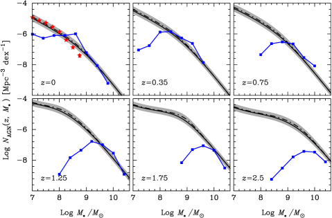
Figure 1.— SMBH mass function of AGNs. Solid and dot-dashed lines are the calculated mass function using Equation (10) with a log-normal and power-law distribution of Eddington ratios, respectively. The shaded areas represent a typical error of $\Delta\log N_{\rm AGN}\approx\pm 0.2$ dex from the AGN bolometric LF of Hopkins et al. (2007). Asterisks in the $z=0$ bin are from Greene & Ho (2007), and squares are from Vestergaard & Osmer (2009), who also compiled the SMBH mass function at $0.025<z<0.5$ from the Bright Quasar Survey. For the sake of a comparison, we superpose it in the $z=0$ bin. Note that the turnover toward the low-mass end of the mass function of Vestergaard & Osmer is due to high survey incompleteness (Kelly et al. 2010).

2. The Continuity Equation of Black Holes

Let $N(t,{M_{\bullet}})$ be the SMBH mass function, including both active and inactive black holes, which specifies the number of black holes per unit comoving volume and per unit mass at cosmic time $t$. Its evolution is described by a continuity equation (e.g., Small & Blandford 1992)

$$\frac{\partial N(t,{M_{\bullet}})}{\partial t}+\frac{\partial}{\partial{M_{\bullet}}}\left[N(t,{M_{\bullet}})\langle\dot{M}_{\bullet}\rangle\right]=S(t,{M_{\bullet}}),$$ (1)

where $\langle\dot{M}_{\bullet}\rangle$ is the mean mass accretion rate for inactive and active SMBHs with mass ${M_{\bullet}}$ at time $t$, and $S(t,{M_{\bullet}})$ is the source term that accounts for black hole mergers. As in most previous works (e.g., Small & Blandford 1992; Yu & Tremaine 2002; Marconi et al. 2004), we neglect black hole mergers, setting $S(t,{M_{\bullet}})=0$. Shankar et al. (2009, 2010) investigated the importance of black hole mergers on the evolution of the SMBH mass function and concluded that the effect of mergers is minor compared with mass accretion. Numerical simulations by Volonteri et al. (2005) and Berti & Volonteri (2008) also verified that mass accretion dominates over mergers in determining the mass growth and spin distribution of black holes.

The radiation power of a SMBH with mass accretion rate $\dot{M}_{\rm acc}$ is $L=\eta\dot{M}_{\rm acc}c^{2}$. Because of radiative losses, the mass growth rate of the SMBH is $\dot{M}_{\bullet}=(1-\eta)\dot{M}_{\rm acc}$, yielding $\dot{M}_{\bullet}=(1-\eta)\lambda L_{\rm Edd}/\eta c^{2}$. Here the Eddington ratio is defined as $\lambda=L/L_{\rm Edd}$, where $L_{\rm Edd}=4\pi G{M_{\bullet}}m_{p}c/\sigma_{\rm T}$, $G$ is the gravitational constant, $m_{p}$ is the proton mass, $c$ is the light speed, and $\sigma_{\rm T}$ is the Thomson electron scattering cross section. With the help of the duty cycle of SMBHs, $\delta(t,{M_{\bullet}})$, the mean mass accretion rate can be written as

$$\langle\dot{M}_{\bullet}\rangle=\delta(t,{M_{\bullet}})\dot{M}_{\bullet}=\delta(t,{M_{\bullet}})\frac{1-\eta}{\eta}\frac{{\bar{\lambda}}(t,{M_{\bullet}})L_{\rm Edd}}{c^{2}},$$ (2)

where $\bar{\lambda}(t,{M_{\bullet}})$ is the mean Eddington ratio determined from observations (see Equation 12 below). The duty cycle is usually defined as

$$\delta(t,{M_{\bullet}})=\frac{N_{\rm AGN}(t,{M_{\bullet}})}{N_{\rm G}(t,{M_{\bullet}})+N_{\rm AGN}(t,{M_{\bullet}})},$$ (3)

where $N_{\rm G}(t,{M_{\bullet}})$ and $N_{\rm AGN}(t,{M_{\bullet}})$ are the SMBH mass functions of galaxies and AGNs, respectively, and, accordingly

$$N(t,{M_{\bullet}})=N_{\rm G}(t,{M_{\bullet}})+N_{\rm AGN}(t,{M_{\bullet}}).$$ (4)

Combining the above equations, we rewrite the continuity equation

$$\frac{\partial N(z,{M_{\bullet}})}{\partial z}=-\frac{{d}t}{{d}z}\frac{\partial}{\partial{M_{\bullet}}}\left[\frac{1-\eta}{\eta}\frac{\bar{\lambda}(z,{M_{\bullet}})L_{\rm Edd}N_{\rm AGN}(z,{M_{\bullet}})}{c^{2}}\right],$$ (5)

where and hereinafter we substitute the cosmic time $t$ with the corresponding redshift $z$. Integrating Equation (5) over $M_{\bullet}^{\prime}$ from ${M_{\bullet}}$ to $\infty$, we obtain the radiative efficiency

$$\eta^{-1}(z,{M_{\bullet}})=1+\frac{c^{2}}{\dot{u}(z,{M_{\bullet}})}\left(\frac{{d}t}{{d}z}\right)^{-1}\frac{\partial}{\partial z}\int^{\infty}_{{M_{\bullet}}}N(z,M_{\bullet}^{\prime}){d}{M_{\bullet}^{\prime}},$$ (6)

where the AGN luminosity density is

$$\dot{u}(z,{M_{\bullet}})=\bar{\lambda}(z,{M_{\bullet}})L_{\rm Edd}N_{\rm AGN}(z,{M_{\bullet}}),$$ (7)

and we use the boundary condition $\dot{u}(z,{M_{\bullet}}\rightarrow\infty)=0$. Equation (6) is the generalized $\eta-$equation of Wang et al. (2009). The underlying rationale of this generalized $\eta-$equation lies in the assumption that mass accretion only increases the SMBH mass, but keeps the SMBH number density conserved. Subsequently, variations of the SMBH number density in the interval $[{M_{\bullet}},\infty]$ should come from the “inflow” of SMBHs through the boundary $M_{\bullet}^{\prime}={M_{\bullet}}$ due to mass accretion. As a result, we obtain the radiative efficiency for SMBHs with any given mass of ${M_{\bullet}}$ from the AGN luminosity density.

To solve Equation (6), it is imperative to obtain three ingredients that appear on the right-hand side: the SMBH mass functions of normal galaxies and AGNs, and the Eddington ratio distribution. In the first paper of this series (Li et al. 2011, Paper I), we have derived the SMBH mass function of normal galaxies out to $z\approx 2$ using the latest galaxy luminosity and stellar mass functions. In what follows, we show in detail how to obtain the SMBH mass function of AGNs from the observed Eddington ratio distribution.

Figure 2.— Mean Eddington ratio as a function of (top) black hole mass and (bottom) redshift.

Figure 3.— Duty cycle as a function of (top) black hole mass and (bottom) redshift.

3. Eddington ratio distributions

Observations thus far have not yet reached a consensus on the observed Eddington ratio distribution, especially at high redshifts. The challenges arise from systematic uncertainties in measuring black hole mass using the virial relation and the flux limit of surveys. However, among earlier studies, two types of Eddington ratio distributions are preferred. Generally, the observed Eddington ratios derived from the bright AGN (quasar) samples exhibit a log-normal distribution (Kollmeier et al. 2006; Shen et al. 2008; Kauffmann & Heckman 2009; Kelly et al. 2010). By contrast, those derived from samples that include fainter sources or low-luminosity AGNs display a power-law distribution and/or an additional log-normal component in the high-Eddington ratio regime (Heckman et al. 2004; Yu et al. 2005; Hopkins & Hernquist 2009; Kauffmann & Heckman 2009; Schulze & Wisotzki 2010). In particular, the peak and dispersion of the log-normal distribution are found to be almost independent of luminosity and redshift (Kollmeier et al. 2006; Shen et al. 2008). Through analysis of the properties of the host galaxies selected from SDSS, Kauffmann & Heckman (2009) argued that in the log-normal regime black holes self-regulate their growth in environments with a plentiful supply of cold gas, so that the Eddington ratio is retained at a universal rate independent of luminosity (black hole mass) and the properties of the host galaxies. By contrast, in the power-law regime the gas has run out and the central black holes are probably being fueled by mass loss from stars in the bulges, thereby appearing as low-luminosity AGNs (Ho, 2009a, b).

With the above lines of observations, we employ two types of Eddington ratio distribution in our calculations. We express the log-normal distribution as

$$P(\lambda)d\log\lambda=\frac{1}{\sqrt{2\pi}\sigma}\exp\left[-\frac{(\log\lambda-\mu)^{2}}{2\sigma^{2}}\right]d\log\lambda,$$ (8)

where $\mu$ is the logarithm of the peak Eddington ratio and $\sigma$ is the dispersion. Below we will show how to determine $\mu$. The dispersion $\sigma$ is found to be inessential to our results, and we set $\sigma=0.3$ (Kollmeier et al. 2006). The power-law distribution is given by

$$P(\lambda)d\log\lambda=C_{0}\left(\frac{\lambda}{\lambda_{0}}\right)^{-\kappa}\exp\left(-\frac{\lambda}{\lambda_{0}}\right)d\log\lambda~{}~{}~{}~{}~{}~{}~{}\lambda>\lambda_{\rm min},$$ (9)

where $C_{0}$ is the normalization, $\lambda_{0}$ is the characteristic ratio, $\kappa$ is the power-law index, and $\lambda_{\rm min}$ is the lower cut-off (Hopkins & Hernquist 2009; see also Cao 2010). According to their feedback-regulated model, Hopkins & Hernquist (2009) suggest typical values of $\lambda_{0}\approx 0.2-0.4$ and $\kappa\approx 0.3-0.8$. In our calculations, we set $\lambda_{0}=0.3$ and $\kappa=0.6$ as fiducial values. Note that for the power-law distribution, a lower cut-off $\lambda_{\rm min}$ is required to completely determine the normalization $C_{0}$. We adjust the values of $\lambda_{\rm min}$ so that the calculated SMBH mass function of AGNs matches the observed one.

Cao & Li (2008) derived the mean Eddington ratio for a given black hole mass and redshift from the observed Eddington ratio distribution. For clarity, we present the details here. The SMBH mass function of AGNs is calculated by combining the observed Eddington ratio distribution and the AGN bolometric LF as

$$N_{\rm AGN}(z,{M_{\bullet}})=\int\Phi(z,L_{\rm bol})\frac{{d}\log L_{\rm bol}}{{d}\log{M_{\bullet}}}P(\lambda){d}\log\lambda,$$ (10)

where $\Phi(z,L_{\rm bol})$ is the AGN bolometric LF. Applying Bayes’ theorem, the Eddington ratio distribution for a given black hole mass ${M_{\bullet}}$ is

$$\omega(z,\lambda|{M_{\bullet}})=\frac{\Phi(z,L_{\rm bol})P(\lambda)}{N_{\rm AGN}(z,{M_{\bullet}})}.$$ (11)

The mean Eddington ratio of AGNs with ${M_{\bullet}}$ at redshift $z$ is

$$\bar{\lambda}(z,{M_{\bullet}})=\int\lambda\omega(z,\lambda|{M_{\bullet}}){d}\log\lambda,$$ (12)

where $\int\omega(z,\lambda|{M_{\bullet}}){d}\log\lambda=1$.

In Figure 1, we compare with observations the SMBH mass function of AGNs calculated by Equation (10) using two types of Eddington distributions. To delineate the evolution of the AGN populations, we adopt Hopkins et al.’s (2007) bolometric LF, which combines a large set of AGN LF measurements in the rest-frame optical, soft and hard X-ray, and near-IR and mid-IR bands, spanning a range of bolometric luminosities from $\sim 10^{42}$ to $10^{49}~{}{\rm erg~{}s^{-1}}$. Greene & Ho (2007) measured the local SMBH mass function of broad-line AGNs from SDSS using standard virial relations. Based on the same method, Vestergaard & Osmer (2009) compiled the SMBH mass function of broad-line AGN samples drawn from the Large Bright Quasar Survey, the Bright Quasar Survey, and SDSS, covering a range of redshift from the local epoch up to $z=5$. Note that the turnover toward the low-mass end of the mass function of Vestergaard & Osmer is due to the incompleteness of the surveys. Kelly et al. (2010) carefully estimated the incompleteness of the SDSS sample of Vestergaard & Osmer and found that it is highly incomplete for ${M_{\bullet}}\lesssim 10^{9}\,M_{\odot}$ at $z>1$. Since these measurements just cover the unobscured population of AGNs, a correction factor has to be applied to Equation (10) to account for such a selection bias before performing this comparison (see Section 4 below). By fine tuning the value of $\mu$ for the log-normal distribution of Eddington ratio, we find that $\mu=-0.6$ produces an AGN SMBH mass function that is in excellent agreement with the observed ones, particularly for the data of Greene & Ho (2007) at $z=0$, as shown in Figure 1. Similarly, a value of $\lambda_{\rm min}=0.1$ for the power-law distribution also gives an almost identical mass function. However, it is probably unphysical that the Eddington ratio for the power-law distribution is cut off at $\lambda_{\rm min}=0.1$. Nevertheless, whichever type of Eddington ratio distribution is used has very little influence on the final results in the sense that the resultant AGN SMBH mass functions are very insensitive to the actual choice (see Figure 1). Hereafter, we only use the log-normal distribution in our calculations.

Figure 2 shows the dependence of the mean Eddington ratio on black hole mass and redshift. We find that the mean Eddington ratio roughly spans values in the range $\sim 0.1-0.3$, slightly increasing with redshift and decreasing with black hole mass. These trends between the mean Eddington ratio and black hole mass and redshift are due to the power-law shape of the AGN LF and the redshift evolution of the slope of the power law. At the same time, we know that nearby massive active galaxies generally contain black holes accreting at an Eddington ratio substantially below unity (e.g., Ho 2008, 2009a). This does not conflict with the present results, considering that local luminous AGNs are quite rare. Moreover, we here focus on efficient accretion phases with high Eddington ratios, during which black hole growth predominately happens (e.g., Hopkins et al. 2006; Xu & Cao 2010).

Figure 4.— Luminosity density $\dot{u}$ (see Equation 7) as a function of redshift, for different black hole masses.

4. Accounting for Compton-thick AGNs

Given the Eddington ratio distribution and AGN bolometric LF, it is trivial to calculate the SMBH mass function for AGNs using Equation (10). However, it is important to note that different bands are subject to different selection biases. Optical LFs miss obscured AGNs (e.g., Bongiorno et al. 2007), while hard X-ray surveys ($\sim 2-10$ keV) can trace only AGNs that are not completely Compton-thick (e.g., Hasinger 2008), namely sources with column densities $N_{\rm H}\lesssim 10^{24}$ cm^-2. Treister et al. (2010) recently presented an evolution model for AGNs hosted by galaxies undergoing major mergers and find that Compton-thick sources play an important role in the mass growth of SMBHs. Meanwhile, evidence is mounting from deep X-ray surveys, in combination with IR surveys, that the population of Compton-thick AGNs with intermediate luminosities is of the same order as that of Compton-thin AGNs (sources with $N_{\rm H}\approx 10^{22}-10^{24}{\rm~{}cm^{-2}}$; e.g., Daddi et al. 2007; Alexander et al. 2008; Fiore et al. 2009; Treister et al. 2009). Population synthesis models of the cosmic X-ray background also predict the existence of a large number of Compton-thick AGNs (e.g., Gilli et al. 2007; Draper & Ballantyne 2009).

How the fraction of Compton-thick AGNs evolves with redshift is not well known. Even the overall evolution of Compton-thin AGNs is in debate. After correcting for selection bias in their hard X-ray-selected AGN sample spanning the redshift range $z=0-4$, Treister & Urry (2006) find that the fraction of obscured AGNs increases with redshift as $(1+z)^{\alpha}$, with $\alpha\approx 0.3-0.5$. Ballantyne et al. (2006), modeling the X-ray background, also report a similar evolution trend of $(1+z)^{0.3}$. However, other studies cast doubt on the redshift evolution of the obscured AGN fraction (Ueda et al. 2003; Dwelly & Page 2006; Gilli et al. 2007; Lamastra et al. 2008). Based on their AGN population model, Gilli et al. (2010) argue that by including a proper $K-$correction an intrinsically constant obscured AGN fraction can also represent the data.

Motivated by the above results, we parameterize the redshift dependence of the fraction of Compton-thick for all AGNs as

$$f_{\rm C}=f_{\rm C,0}(1+z)^{\alpha},$$ (13)

with $f_{\rm C,0}\approx 0.3$ and $\alpha\approx 0.3$. Here we determine $f_{\rm C,0}$ by assuming that the local fraction of obscured (Compton-thin and Compton-thick) to unobscured AGNs is $\sim 3:1$ (Treister & Urry 2006), and that there is an equal abundance of Compton-thin and Compton-thick sources. As described later, our final results are quite insensitive to the value of $\alpha$; therefore, we set $\alpha=0.3$, consistent with Treister & Urry (2006) and Ballantyne et al. (2006). On the other hand, it is well established that the obscured fraction of Compton-thin AGNs decreases with luminosity (Ueda et al. 2003; La France et al. 2005; Hasinger 2008). The dependence of obscuration on luminosity for Compton-thick AGNs, however, is still poorly understood. We neglect this effect, but we discuss the implications in Section 6.2.3.

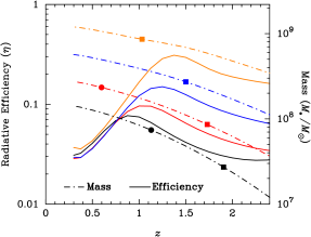
Figure 5.— Evolution of black hole mass (dot-dashed lines) and associated radiative efficiency (solid lines) as a function of redshift. The initial masses are set to $10^{7}$, $10^{7.5}$, $10^{8}$, and $10^{8.5}$ $M_{\odot}$ at redshift $z_{0}=2.5$. The symbols, squares and circles, indicate when the black hole mass has $e$-folded once and twice, respectively.

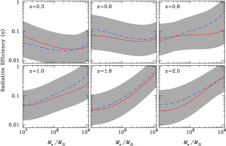
Figure 6.— Radiative efficiency as a function of black hole mass at different redshifts. Solid lines and dot-dashed lines are the efficiency using the SMBH mass function derived from the galaxy luminosity and stellar mass function, respectively. Shaded areas denote typical errors of $\Delta\log\eta=\pm$0.5 dex from SMBH mass function and AGN LF.

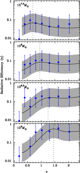
Figure 7.— Radiative efficiency evolution for different black hole masses. Solid lines and data points are the efficiency using the SMBH mass function derived from the galaxy luminosity and stellar mass function, respectively. Shaded areas and error bars denote typical errors of $\Delta\log\eta=\pm$0.5 dex from the SMBH mass function and AGN LF. Vertical dotted lines represent the redshift below which the efficiency begins to decline.

5. Episodes of SMBH Growth

With the AGN SMBH mass function determined from the previous sections, we can calculate the AGN duty cycle, as shown in Figure 3. At low redshifts, the duty cycle decreases with increasing black hole mass, indicating that the fraction of galaxies that are active also declines with mass (Greene & Ho 2007; Shankar 2009). Conversely, as a consequence of the cosmic downsizing of AGN activity, at high redshifts the duty cycle reverses trend and increases with black hole mass. Duty cycles for $10^{7}\,M_{\odot}$ and $10^{9}\,M_{\odot}$ black hole are $\delta\approx 4\times 10^{-3}$ and $\sim 8\times 10^{-4}$ at $z=0$, respectively, but rise up to $\sim 0.06$ and $\sim 0.5$ by $z=2$. As shown in the bottom panel of Figure 3, the active fraction of all black holes increases significantly from $\sim 10^{-3}$ at $z=0$ to $\sim 0.1$ at $z=2$, in concert with the feature of AGN LF that displays a rapid rise up till $z=2$ (see also Wang et al. 2006).

With the duty cycle determined, the active time of AGNs is simply given by $\tau(z,{M_{\bullet}})=\delta(z,{M_{\bullet}})H(z)^{-1}$, where $H(z)$ is the Hubble parameter at redshift $z$ (Peacock 1999). As a result, the active time of AGNs is of the order of $\sim 10^{7}$ yr in the local Universe and $\sim 10^{8}$ yr at $z=2$. This is consistent with the observational estimates from other methods (see Martini 2004 for a review).

Figure 4 illustrates the AGN luminosity density $\dot{u}(z,{M_{\bullet}})$, defined by Equation (7), and its variation with redshift for different black hole masses. Since the mean Eddington ratio is approximately constant over black hole mass and redshift, $\dot{u}(z,{M_{\bullet}})$ just reflects the evolution of the AGN SMBH mass function. Again, the behavior of cosmic downsizing is evident: more massive active black holes reach their maximum number density earlier than less massive ones.

With the mean accretion rate $\langle\dot{M}_{\bullet}\rangle$, we can trace the SMBH growth history since redshift $z_{0}$ as

$${M_{\bullet}}(z)=M_{0}+\int_{z_{0}}^{z}\left\langle\dot{M}_{\bullet}\left[z^{\prime},{M_{\bullet}}(z^{\prime})\right]\right\rangle\frac{dt}{dz^{\prime}}dz^{\prime},$$ (14)

where $M_{0}$ is the initial black hole mass at redshift $z_{0}$. Figure 5 plots the growth history of black holes with initial masses $10^{7}$, $10^{7.5}$, $10^{8}$, and $10^{8.5}$ $M_{\odot}$ at $z_{0}=2.5$. The symbols (squares and circles) indicate when the black hole mass has $e$-folded once and twice. For a hole with an initial mass of $10^{7}\,M_{\odot}$, it grows to $\sim 1.5\times 10^{8}\,M_{\odot}$ at $z\approx 0.3$, $e$-folding roughly 3 times. A $10^{8.5}\,M_{\odot}$ hole grows just to $\sim 1.0\times 10^{9}\,M_{\odot}$ at $z\approx 0.3$, $e$-folding only once. Recall that the $e$-folding time is quantified by the Salpeter (1964) time

$$t_{\rm Sal}=\frac{\eta}{(1-\eta)\bar{\lambda}}\frac{c\sigma_{\rm T}}{4\pi Gm_{p}}=2.3\times 10^{8}\left(\frac{10\eta}{1-\eta}\right)\left(\frac{\bar{\lambda}}{0.2}\right)^{-1}{~{}\rm yr}.$$ (15)

It is obvious that the $e$-folding time scales in proportion to the radiative efficiency. The decline of radiative efficiency makes black hole growth possible, especially for low-mass black holes at low redshift, considering that the AGN life time is of the order of $10^{7}$ yr at that epoch (see also the discussions of King & Pringle 2006; Netzer & Trakhtenbrot 2007; Netzer et al. 2007).

An intriguing issue that has attracted much attention over the years is what is the mass range of seed black holes and how they grow to present-day SMBHs (e.g., Volonteri et al. 2008; Wang et al. 2008). In principle, an extrapolation of the present approach to much higher redshifts, say $z\gtrsim 10$, may be helpful to place constraints on the properties of seed black holes. This is beyond the scope of the present paper, and we defer this investigation to future work.

6. SMBH Spins

6.1. Evolution of the Radiative Efficiency

In Figure 6 we present the radiative efficiency, calculated using Equation (6), as a function of SMBH mass, using the SMBH mass function derived from both the galaxy LF and the galaxy stellar mass function. Shaded areas represent typical errors of $\Delta\log\eta=\pm 0.5$ dex from the SMBH mass function ($\sim 0.3$ dex) and AGN LF ($\sim 0.2$ dex). We find that at low redshifts (e.g., $z\approx 0.3$) SMBH of all masses are accreting material with a relatively low radiative efficiency. At high redshifts (e.g., $z\approx 1-2$), although the uncertainties are large, the radiative efficiency generally increases with black hole mass. A rough correlation is $\eta\propto M_{\bullet}^{\gamma}$, with $\gamma\approx 0.5$. Indeed, Cao & Li (2008) argued on the basis of the Sołtan argument that the radiative efficiency should increase with black hole mass so as to guarantee that the mass function of local relic SMBHs matches the mass function of galaxies. Previous studies, assuming a fixed radiative efficiency over black hole mass and redshift, concluded that $\eta\approx 0.1$ (e.g., Yu & Tremaine 2002; Marconi et al. 2004). The values of the radiative efficiency we obtain here are consistent with this average value.

The redshift dependence of the radiative efficiency is plotted in Figure 7 for different black hole masses. Solid lines show the results obtained using the SMBH mass function derived from the galaxy LF, while the superposed data points make use of the SMBH mass function derived from the galaxy stellar mass function, computed for specific redshift bins. Again, shaded areas and error bars represent typical errors of $\Delta\log\eta=\pm 0.5$ dex. For high-mass black holes ($M_{\bullet}\gtrsim 10^{8.5}\,M_{\odot}$), the radiative efficiency maintains a high value of $\eta\approx 0.3$ at $z\approx 2$, but then strongly declines toward lower redshifts. The radiative efficiency for ${M_{\bullet}}\approx 10^{9}\,M_{\odot}$ at $z\approx 2$ marginally exceeds the maximum efficiency of $\eta\approx 0.4$ allowed for extreme Kerr black holes. This may arise from the unrealistic treatment of the mean Eddington ratio distribution beyond a black hole mass of $10^{9}\,M_{\odot}$. Another cause may be an overestimate of the correction factor for Compton-thick AGNs in Equation (13), if the factor is generally anti-correlated with luminosity. For low-mass black holes, the evolution is more complicated. The radiative efficiency appears to plateau at $z\approx 1-2$ and then decreases dramatically toward $z=0$. Recently, Wang et al. (2009) obtained the average radiative efficiency for black hole masses $M_{\bullet}\gtrsim 10^{8.2}\,M_{\odot}$ with redshift $z<2$. They found a similarly rapid decrease of $\eta$ from $z\approx 2$ to the local epoch (see their Figure 2a).

Figure 5 shows how the black hole mass and the associated radiative efficiency evolve over time. Interestingly, there exists a peak in the efficiency curve: for a given initial mass at redshift $z=2.5$, the efficiency gently rises to a local maximum, and then sharply falls off. The rise of the efficiency during black hole growth is due to the positive correlation between efficiency and mass, as shown in Figure 6, while the subsequent decline is due to the systematic decrease of the efficiency toward low redshifts. It seems that the efficiency evolution can be characterized by two regimes, one during which the efficiency increases and another during which it decreases.

6.2. Evolution of SMBH Spins

If the standard accretion disk model applies to the AGNs under consideration, we can elucidate their spin evolution through the radiative efficiency obtained above (e.g., Thorne 1974). Since black holes gain their mass predominately during their quasar phase (e.g., Hopkins et al. 2006; Xu & Cao 2010), the standard accretion disk model is quite a reasonable approximation. From Figure 6, it is apparent that at high redshifts ($z\gtrsim 1$) black hole spin increases with mass. At low redshifts the dependence of spin on mass seems reversed, although large uncertainties prohibit us from reaching a firm conclusion. Volonteri et al. (2007) have drawn a connection between black hole spin and galactic morphology and argued that SMBHs in elliptical galaxies possess higher spins than those in spiral galaxies. Such a morphology-related spin distribution has been used to explain the observed radio-loudness bimodality in nearby AGNs (e.g., Sikora et al. 2007). Our results at $z\approx 0.3-0.6$ are not qualitatively consistent with this scenario. One possible explanation for this inconsistency is that radio-loud galaxies comprise only a tiny fraction of the galaxy population, whereas our results pertain to a global average of all galaxies. Moreover, our current approach is unable to constrain the dispersion of the spin distribution at any given redshift or mass.

Most importantly, Figure 7 shows that high-mass black holes begin to spin down earlier than low-mass black holes. To guide the eye, the vertical dotted lines in the figure mark the redshift below which the efficiency begins to decline. Recalling the cosmic downsizing of AGN activity, there appears to be a connection between black hole spin and accretion. Indeed, if random accretion plays a role in black hole growth, spin evolution inevitably follows cosmic downsizing just as AGN activity does, since high-mass black holes become active earlier and hence are spun down earlier by random accretion. However, we observe two regimes in the evolution of the radiative efficiency: SMBHs first spin up, and then down. This indicates that more complex accretion scenarios need to be explored. We return to this point in Section 7.

6.3. Influence of Uncertainties

We explore the reliability of the radiative efficiencies in light of some of the assumptions used in our calculations.

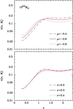
Figure 8.— Influences of the observed Eddington ratio distribution on radiative efficiency for black holes with mass ${M_{\bullet}}=10^{8.5}\,M_{\odot}$. The dependence on the mean ($\mu$) and dispersion ($\sigma$) of the distribution is illustrated in the top and bottom panels, respectively.

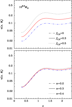
Figure 9.— Influences of the fraction of Compton-thick AGNs on radiative efficiency for black holes with mass ${M_{\bullet}}=10^{8.5}\,M_{\odot}$. The dependence on the normalization ($f_{\rm C,0}$) and redshift dependence ($\alpha$) of the Compton-thick fraction (see Equation 13) is illustrated in the top and bottom panels, respectively.

6.3.1 SMBH Mass Function of Galaxies

The SMBH mass function is a crucial input because it determines the mass growth rate in Equation (6). In Paper I, we derived the SMBH mass function of galaxies out to redshift $z\approx 2$ using the latest luminosity and stellar mass functions of field galaxies to constrain the masses of their spheroids. SMBH masses were inferred through a locally calibrated empirical correlation between black hole mass and spheroid mass. The SMBH mass functions derived from the galaxy luminosity and stellar mass functions show very good agreement, both in shape and in normalization, testifying to the robustness of our results. After carefully examining various sources of uncertainties, we found that the total uncertainties on the SMBH mass function are generally within $\sim 0.3$ dex, and possibly even smaller for lower mass black holes (see Paper I for details). As a consequence, uncertainties in the SMBH mass function introduce an uncertainty less than $\sim 0.3$ dex to the resultant radiative efficiency.

6.3.2 Eddington Ratio Distributions

The observed distribution of Eddington ratios is described as log-normal, independent of luminosity and redshift (e.g., Kollmeier et al. 2006; Shen et al. 2008). Such a distribution may be realistic in the context of a self-regulation model for accretion of black holes embedded in a gas-rich environment (Kauffmann & Heckman 2009). To assess its impact on our results, we calculate the radiative efficiency for three values of the mean Eddington ratio (logarithmic values $\mu=-0.4,-0.6,$ and $-0.8$) and its dispersion ($\sigma$ = 0.2, 0.3, and 0.4) for ${M_{\bullet}}=10^{8.5}\,M_{\odot}$ (Figure 8). We find that $\mu$ does have a mild impact on the redshift position where black hole spin begins to decline: smaller $\mu$ results in a later decrease of spin. However, in comparison with Figure 7, the adopted uncertainty of $\Delta\mu=\pm 0.2$ does not alter the overall cosmic downsizing behavior for the spin evolution. Future systematic studies should try to directly constrain the intrinsic Eddington ratio distribution for a given black hole mass, instead of inferring it from the observed Eddington ratio distribution combined with the AGN LF. The dispersion of the log-normal distribution $\sigma$ has only a very minor influence on the radiative efficiency.

6.3.3 Compton-thick AGNs

We adopt a simple, redshift-dependent correction factor to account for the selection bias of Compton-thick AGNs in Hopkins et al.’s (2007) bolometric LFs (Equation 13). Its possible dependence on luminosity is neglected. From Equation (6), it is apparent that a higher correction factor would enhance the energy density and therefore lead to a larger radiative efficiency (see also Martínez-Sansigre & Taylor 2009). By analogy, if obscuration anti-correlates with luminosity, the radiative efficiency of low-mass black holes will be reduced. This will influence the relation between spin and mass obtained in Figure 6. Unfortunately, the overall luminosity dependence of the fraction of Compton-thick AGNs remains unsettled still (e.g., see Gilli et al. 2010), precluding us from applying a rigorous treatment. Figure 9 shows the influence of the correction for Compton-thick AGNs on the radiative efficiency for $10^{8.5}\,M_{\odot}$ holes. The results are significantly affected by the normalization factor $f_{\rm C,0}$, but they are quite insensitive to the redshift parameter $\alpha$. In any case, the overall evolution trend of radiative efficiency is qualitatively preserved.

6.3.4 SMBH Mergers

As in most previous works, we neglect the term for black hole mergers in the continuity equation and, motivated by Sołtan’s argument, assume that black hole growth is mainly driven by baryon accretion. As mentioned above, previous studies show that mass accretion dominates over mergers in determining the mass growth and spin distribution of black holes (Berti & Volonteri 2008; King et al. 2008). Shankar et al. (2009, 2010), using theoretically predicted merger rates from hierarchical structure formation models, also conclude that the effect of mergers is minor compared with mass accretion. However, based on a semi-analytic model of hierarchical galaxy formation and evolution incorporating black hole growth, Fanidakis et al. (2011b) recently showed that mergers do contribute significantly to the final black hole mass for high-mass black holes (e.g., ${M_{\bullet}}\gtrsim 10^{9}\,M_{\odot}$). Both of these calculations are subject to the uncertainties of the adopted recipes for merger rates of black holes, which are not well understood yet.

6.4. Comparison with Previous Results

Several recent parallel studies have attempted to observationally estimate SMBH radiative efficiency or spin. Directly starting from the definition of radiative efficiency, Davis & Laor (2011) obtained the efficiencies of individual sources in a sample of 80 Palomar-Green quasars using the bolometric luminosity and the accretion rate determined from accretion disk model spectral fits. They found an average $\eta\approx 0.1$ and a trend of increasing efficiency with increasing black hole mass (see also Raimundo et al. 2011). The redshift range of their sample is confined to $z\leq 0.5$. The correlation of the radiative efficiency with black hole mass found by Davis & Laor (2011) is not completely compatible with our results (i.e. redshift bins $z=0.3$ and $0.6$ in Figure 6), although both calculations suffer from large uncertainties.

Another common but highly model-dependent way to constrain SMBH spin is through the jet/radio power of radio-loud AGNs. In a series of works, Daly (2009a, b, 2011) analyzed the radio beam power using large samples of extended radio sources and then determined the black hole spin with the aid of a correlation between the beam power and spin. Their results generally suggest that black hole spin in radio sources decreases moderately from redshift $z\approx 2$ to the local Universe. Conversely, assuming that the efficiency of jet production is uniquely dependent on black hole spin, Martínez-Sansigre & Rawlings (2011a) inferred the spin distribution by modeling the radio luminosity function of radio sources with high- and low-excitation narrow emission lines. They found that the best-fit spins show a bimodal distribution, whose peaks correspond to the high- and low-excitation radio sources, respectively. In particular, their model favors a trend in which the typical black hole spin increases slowly toward low redshift since $z\approx 3$. A follow-up study by Martínez-Sansigre & Rawlings (2011b), based on a similar method, gave an even steeper evolutionary trend of black hole spin from $z\approx 1$ to $z\approx 0$. In terms of spin evolution, our results obtained here are qualitatively consistent with those of Daly (2009a, b, 2011). However, the stark differences between the results of Daly and Martínez-Sansigre & Rawlings suggest that approaches that rely on the radio power to deduce black hole spin should be treated with caution.

A number of semi-analytic models of galaxy formation have attempted to incorporate the growth of black holes and track their spin evolution. Although the prescriptions for implementing gas fueling from large to small scales are uncertain and differ from study to study, there is broad consensus that the final black hole spin strongly depends on the assumed configuration of the angular momentum of the accreted gas (Volonteri et al. 2005; Berti & Volonteri 2008; Lagos et al. 2009; Fanidakis et al. 2011a, b). The models of Lagos et al. (2009) and Fanidakis et al. (2011a) predict that the average black hole spin increases with mass. At first glance, this is qualitatively consistent with our results at high redshifts. However, they ascribe their results to the major mergers of black holes, which exclusively produce remnant holes with high spin (Hughes & Blandford 2003). Our calculations, by contrast, explicitly neglect black hole mergers and assume that mass accretion dominates black hole growth. We contend that this is a reasonable assumption. Indeed, many recent studies cast doubt on the importance of the role played by major mergers in the evolution of galaxies in general (e.g., Naab et al. 2009; Taylor et al. 2010; Williams et al. 2011, and references therein), and active galaxies in particular (e.g., Cisternas et al. 2011; Rosario et al. 2011, and references therein), especially for redshifts below $z\approx 2$.

7. Implications on Accretion Scenarios

Two possible accretion scenarios affect black hole spins (e.g., King & Pringle 2006; Berti & Volonteri 2008; King et al. 2008; Martínez-Sansigre & Taylor 2009). (1) SMBHs grow through prolonged accretion episodes, during which the holes are quickly spun up to their maximum rate by capturing material with constant angular momentum (Thorne 1974). (2) SMBHs grow via many short-lived and random accretion episodes, acquiring gas with initially random orientations with respect to the rotation axis of the hole, which efficiently cancels out the net angular momentum and leads to moderately rotating holes (King et al. 2008; Wang et al. 2009; Li et al. 2010). As in Wang et al. 2009, we appeal to episodic, short-lived random accretion as the driving mechanism to explain the intense decline of black hole spins since $z\approx 1-2$. The situation may be fundamentally different at higher redshifts ($z\gtrsim 2$), when galaxies are characteristically more gas-rich and major mergers are more prevalent. At these earlier epochs, it is natural to expect black hole growth to be more dominated by episodes of prolonged accretion, leading to high spins and high radiative efficiencies, particularly for high-mass systems. We propose that this is the fundamental explanation for the two regimes of spin evolution seen in our analysis (Figure 5): black holes spin up by prolonged accretion, possibly aided by major mergers, up to $z\approx 2$, and thereafter spin down by episodic accretion driven by minor mergers and internal secular processes.

Random accretion inevitably leaves the accretion disk misaligned with respect to the spin axis of the black hole. In this case, the presence of viscosity combined with Lense-Thirring precession will induce the inner portion of the disk to align or anti-align its orbital angular momentum with that of the black hole out to a transition radius, beyond which the disk retains its initial inclination (so-called Bardeen-Petterson effect; Bardeen & Petterson 1975). The characteristic extension of the transition radius and the time scale for alignment or anti-alignment depend on the black hole mass and spin (e.g., Pringle 1992; King et al. 2005). The Bardeen-Petterson effect may exert a vital influence on the spin evolution of the black hole (e.g., see also Perego et al. 2009). We defer a complete study of the relation between spin and mass during multiple episodes of black hole growth to a third paper of this series (Y.-R. Li et al. 2012, in preparation).

8. Conclusions

We derive the mass-dependent cosmological evolution of the radiative efficiency for mass accretion, which, according to the standard model of accretion disks, can be used as a surrogate to estimate the black hole spin. The calculated radiative efficiency generally increases with black hole mass, roughly as $\eta\propto M_{\bullet}^{0.5}$ at high redshifts ($z\gtrsim 1$), but the trend reverses at low redshifts, such that $\eta$ increases with decreasing $M_{\bullet}$. High-mass black holes ($M_{\bullet}\gtrsim 10^{8.5}\,M_{\odot}$) maintain a high efficiency ($\eta\approx 0.3$) at $z\approx 2$, which then declines strongly toward lower redshifts. The evolutionary pattern for lower mass black holes is somewhat more complicated, but it is generally consistent with the radiative efficiency decreasing since $z\approx 1$ in like manner. Most importantly, we find that the efficiency of high-mass black holes begins to decline earlier than that of low-mass black holes, qualitatively similar to the cosmic downsizing of AGN activity. Assuming that the radiative efficiency provides an effective indirect measure of the black hole spin, we propose the following picture for the spin evolution of SMBHs:

• The evolution of the spin of the black hole tracks the growth history of its mass and can be characterized by two regimes: an initial phase of mass accumulation from prolonged accretion that spins up the hole, followed by a period of random, episodic accretion that spins down the hole toward lower redshifts.

• The evolution of the spin, like the global pattern of AGN activity, exhibits “cosmic downsizing”. Relative to lower mass black holes, high-mass systems gain their masses earlier, reach the peak of their AGN activity earlier, and begin to spin down earlier. Random accretion dominates their evolution below $z\approx 2$, whereas lower mass holes transition to this phase later, at $z\approx 1$.

Finally, it is worth listing the principal assumptions used in our calculations, on which better observational constraints would be welcomed: (1) the scaling relation between SMBH mass and the mass of the bulge of the host galaxy applies over the redshift range $0<z<2$, so that the SMBH mass function can be inferred from the galaxy luminosity and stellar mass functions; (2) black holes gain their mass through baryon accretion and black hole mergers are negligible; (3) black hole growth mainly occurs during quasar phases characterized by universal Eddington ratio distribution; (4) the number of Compton-thick AGNs is comparable to that of Compton-thin AGNs, and they both have a similar Eddington ratio distribution as that of unobscured sources. Future deep multiwavelength surveys are awaited to test and refine these assumptions.

References

- Alexander et al. [2008] Alexander, D. M., Chary, R.-R., Pope, A., et al. 2008, ApJ, 687, 835
- Babić et al. [2007] Babić, A., Miller, L., Jarvis, M. J., et al. 2007, A&A, 474, 755
- Ballantyne et al. [2006] Ballantyne, D. R., Everett, J. E. & Murray, N. 2006, ApJ, 639, 740
- Bardeen & Petterson [1975] Bardeen, J. M., & Petterson, J. A. 1975, ApJ, 195, L65
- Berti & Volonteri [2008] Berti, E., & Volonteri, M. 2008, ApJ, 684, 822
- Bongiorno et al. [2007] Bongiorno, A., Zamorani, G., Gavignaud, I., et al. 2007, A&A, 472, 443
- Cao [2010] Cao, X. 2010, ApJ, 725, 388
- Cao & Li [2008] Cao, X.-W., & Li, F. 2008, MNRAS, 390, 561
- Chokshi & Turner [1992] Chokshi, A., & Turner, E. 1992, MNRAS, 259, 421
- Cirasuolo et al. [2010] Cirasuolo, M., McLure, R. J., Dunlop, J. S., et al. 2010, MNRAS, 401, 1166
- Cisternas et al. [2011] Cisternas, M., Jahnke, K., Inskip, K. J., et al. 2011, ApJ, 726, 57
- Daddi et al. [2007] Daddi, E., Alexander, D. M., Dickinson, M., et al. 2007, ApJ, 670, 173
- Daly [2011] Daly, R. A. 2011, MNRAS, 395
- Daly [2009a] Daly, R. A. 2009a, ApJ, 691, L72
- Daly [2009b] Daly, R. A. 2009b, ApJ, 696, L32
- Davis & Laor [2011] Davis, S. W., & Laor, A. 2011, ApJ, 728, 98
- Draper & Ballantyne [2009] Draper, A. R., & Ballantyne, D. R. 2009, ApJ, 707, 778
- Dwelly & Page [2006] Dwelly, T., & Page, M. J. 2006, MNRAS, 372, 1755
- Elvis et al. [2002] Elvis, M., Risaliti, G., & Zamorani, G. 2002, ApJ, 565, L75
- Fabian & Iwasawa [1999] Fabian, A. C., & Iwasawa, K. 1999, MNRAS, 303, L34
- Fanidakis et al. [2011a] Fanidakis, N., Baugh, C. M., Benson, A. J., et al. 2011a, MNRAS, 410, 53
- Fanidakis et al. [2011b] Fanidakis, N., Baugh, C. M., Benson, A. J., et al. 2011b, MNRAS, 419, 2979
- Fiore et al. [2009] Fiore, F., Puccetti, S., Brusa, M., et al. 2009, ApJ, 693, 447
- Gilli et al. [2007] Gilli, R., Comastri, A., & Hasinger, G. 2007, A&A, 463, 79
- Gilli et al. [2010] Gilli, R., Comastri, A., Vignali, C., Ranalli, P., & Iwasawa, K. 2010, in AIP Conf. Proc., X-ray Astronomy 2009: Present Status, Multiwavelength Approach and Future Perspectives, ed. A. Comastri, M. Cappi, & L. Angelini (Melville, NY: AIP), arXiv:1004.2412
- Greene & Ho [2007] Greene, J. E., & Ho, L. C. 2007, ApJ, 667, 131
- Hasinger [2008] Hasinger, G. 2008, A&A, 490, 905
- Heckman et al. [2004] Heckman, T. M., Kauffmann, G., Brinchmann, J., et al. 2004, ApJ, 613, 109
- Ho [2008] Ho, L. C. 2008, ARA&A, 46, 475
- Ho [2009a] Ho, L. C. 2009a, ApJ, 699, 626
- Ho [2009b] Ho, L. C. 2009b, ApJ, 699, 638
- Hopkins & Hernquist [2009] Hopkins, P. F., & Hernquist, L. 2009, ApJ, 698, 1550
- Hopkins et al. [2006] Hopkins, P. F., Narayan, R., & Hernquist, L. 2006, ApJ, 643, 641
- Hopkins et al. [2007] Hopkins, P. F., Richards, G. T., & Hernquist, L. 2007, ApJ, 654, 731
- Hughes & Blandford [2003] Hughes, S. C. & Blandford, R. D. 2003, ApJ, 585, L101
- Kauffmann & Heckman [2009] Kauffmann, G., & Heckman, T. M. 2009, MNRAS, 397, 135
- Kelly et al. [2010] Kelly, B. C., Vestergaard, M., Fan, X., et al. 2010, ApJ, 719, 1315
- King et al. [2005] King, A. R., Lubow, S. H., Ogilvie, G. I., & Pringle, J. E. 2005, MNRAS, 363, 49
- King & Pringle [2006] King, A. R., & Pringle, J. E. 2006, MNRAS, 373, L90
- King et al. [2008] King, A. R., Pringle, J. E., & Hofmann, J. A. 2008, MNRAS, 385, 1621
- Kollmeier et al. [2006] Kollmeier, J. A., Onken, C. A., Kochanek, C. S., et al. 2006, ApJ, 648, 128
- Labita et al. [2009a] Labita, M., Decarli, R., Treves, A., & Falomo, R. 2009a, MNRAS, 396, 1537
- Labita et al. [2009b] Labita, M., Decarli, R., Treves, A., & Falomo, R. 2009b, MNRAS, 399, 2099
- La France et al. [2005] La Franca, F., Fiore, F., Comastri, A., et al. 2005, ApJ, 635, 864
- Lagos et al. [2009] Lagos, C. D. P., Padilla, N. D., & Cora, S. A. 2009, MNRAS, 395, 625
- Lamastra et al. [2008] Lamastra, A., Perola, G. C., & Matt, G. 2008, A&A, 487, 109
- Li et al. [2011] Li, Y.-R., Ho, L. C., & Wang, J.-M. 2011, ApJ, 742, 33 (Paper I)
- Li et al. [2010] Li, Y.-R., Wang, J.-M., Yuan, Y.-F., Hu, C., & Zhang, S. 2010, ApJ, 710, 878
- Marconi et al. [2004] Marconi, A., Risaliti, G., Gilli, R., Hunt, L. K., Maiolino, R., & Salvati, M. 2004, MNRAS, 351, 169
- Martínez-Sansigre & Rawlings [2011a] Martínez-Sansigre, A., & Rawlings, S. 2011a, MNRAS, 414, 1937
- Martínez-Sansigre & Rawlings [2011b] Martínez-Sansigre, A., & Rawlings, S. 2011b, MNRAS, 418, L84
- Martínez-Sansigre & Taylor [2009] Martínez-Sansigre, A., & Taylor, A. M. 2009, 692, 964
- Martini [2004] Martini, P. 2004, in Carnegie Observatories Astrophysics Series, Vol. 1: Coevolution of Black Holes and Galaxies, ed. L. C. Ho (Cambridge: Cambridge Univ. Press), 169
- Merloni & Heinz [2008] Merloni, A., & Heinz, S. 2008, MNRAS, 388, 1011
- Naab et al. [2009] Naab, T., Johansson, P. H., & Ostriker, J. P. 2009, ApJ, 699, L178
- Netzer et al. [2007] Netzer, H., Lira, P., Trakhtenbrot, B., Shemmer, O., & Cury, I. 2007, ApJ, 671, 1256
- Netzer & Trakhtenbrot [2007] Netzer, H., & Trakhtenbrot, B. 2007, ApJ, 654, 754
- Peacock [1999] Peacock, J. A. 1999, Cosmological Physics (Cambridge: Cambridge Univ. Press)
- Perego et al. [2009] Perego, A., Dotti, M., Colpi, M., & Volonteri, M. 2009, MNRAS, 399, 2249
- Pringle [1992] Pringle, J. E. 1992, MNRAS, 258, 811
- Raimundo et al. [2011] Raimundo, S. I., Fabian, A. C., Vasudevan, R. V., Gandhi, P., & Wu, J. 2011, MNRAS, 419, 2529
- Rosario et al. [2011] Rosario, D. J., Mozena, M., Wuyts, S., et al. 2011, ApJ, in press (arXiv:1110.3816)
- Salpeter [1964] Salpeter, E. E. 1964, ApJ, 140, 796
- Schulze & Wisotzki [2010] Schulze, A., & Wisotzki, L. 2010, A&A, 516, A87
- Shankar [2009] Shankar, F. 2009, New Astron. Rev., 53, 57
- Shankar et al. [2010] Shankar, F., Crocce, M., Miralda-Escudé, J., Fosalba, P., & Weinberg, D. H. 2010, ApJ, 718, 231
- Shankar et al. [2004] Shankar, F., Salucci, P., Granato, G. L., De Zotti, G., & Danese, L. 2004, MNRAS, 354, 1020
- Shankar et al. [2009] Shankar, F., Weinberg, D. H., & Miralda-Escudé, J. 2009, ApJ, 690, 20
- Shapiro [2005] Shapiro, S. L. 2005, ApJ, 620, 59
- Shen et al. [2008] Shen, Y., Greene, J. E., Strauss, M. A., Richards, G. T., & Schneider, D. P. 2008, ApJ, 680, 169
- Sikora et al. [2007] Sikora, M., Stawarz, L., & Lasota, J.-P. 2007, ApJ, 658, 815
- Small & Blandford [1992] Small, T. A., & Blandford, R. D. 1992, MNRAS, 259, 725
- Sołtan [1982] Sołtan, A. 1982, MNRAS, 200, 115
- Taylor et al. [2010] Taylor, E. N., Franx, M., Glazebrook, K., et al. 2010, ApJ, 720, 723
- Thorne [1974] Thorne, K. S. 1974, ApJ, 191, 507
- Treister et al. [2010] Treister, E., Natarajan, P., Sanders, D. B., Urry, C. M., Schawinski, K., & Kartaltepe, J. 2010, Science, 328, 600
- Treister & Urry [2006] Treister, E., & Urry, C. M. 2006, ApJ, 652, L79
- Treister et al. [2009] Treister, E., Cardamone, C. N., Schawinski, K., et al. 2009, ApJ, 706, 535
- Ueda et al. [2003] Ueda, Y., Akiyama, M., Ohta, K., & Miyaji, T. 2003, ApJ, 589, 886
- Wang et al. [2008] Wang, J.-M., Chen, Y.-M., Yan, C.-S., & Hu, C. 2008, ApJ, 673, L9
- Wang et al. [2006] Wang, J.-M., Chen, Y.-M., & Zhang, F. 2006, ApJ, 647, L17
- Wang et al. [2009] Wang, J.-M., Hu, C., Li, Y.-R., et al. 2009, ApJ, 697, L141
- Williams et al. [2011] Williams, R. J., Quadri, R. F., & Franx, M. 2011, ApJ, 738, L25
- Vestergaard & Osmer [2009] Vestergaard, M., & Osmer, P. S. 2009, ApJ, 699, 800
- Volonteri et al. [2008] Volonteri, M., Lodato, G., & Natarajan, P. 2008, MNRAS, 383, 1079
- Volonteri et al. [2005] Volonteri, M., Madau, P., Quataert, E., & Rees, M. J. 2005, ApJ, 667, 704
- Volonteri et al. [2007] Volonteri, M., Sikora, M., & Lasota, J.-P. 2007, ApJ, 667, 704
- Xu & Cao [2010] Xu, Y.-D., & Cao, X. 2010, ApJ, 716, 1423
- Yu et al. [2005] Yu, Q., Lu, Y., & Kauffmann, G. 2005, ApJ, 634, 901
- Yu & Tremaine [2002] Yu, Q., & Tremaine, S. 2002, MNRAS, 335, 965