Condensate deformation and quantum depletion of Bose-Einstein condensates in external potentials

Abstract

The one-body density matrix of weakly interacting, condensed bosons in external potentials is calculated using inhomogeneous Bogoliubov theory. We determine the condensate deformation caused by weak external potentials on the mean-field level. The momentum distribution of quantum fluctuations around the deformed ground state is obtained analytically, and finally the resulting quantum depletion is calculated. The depletion due to the external potential, or potential depletion for short, is a small correction to the homogeneous depletion, validating our inhomogeneous Bogoliubov theory. Analytical results are derived for weak lattices and spatially correlated random potentials, with simple, universal results in the Thomas-Fermi limit of very smooth potentials.

1 Penrose-Onsager criterion and Bogoliubov theory for inhomogeneous condensates

The phenomenon of Bose-Einstein condensation (BEC) plays a pivotal role in condensed-matter physics. In recent years, the unique experimental possibilities offered by dilute ultracold atomic gases have triggered a renewed interest in Bose-Einstein condensates. These are loaded into external potentials of a large variety, ranging from simple harmonic traps to increasingly complicated optical lattices, all the way to random potentials [1, 2, 3]. The more complicated the confining potentials are, the greater is the challenge to tell the condensate from the excitations, both quantum and thermal. Yet, to be able to distinguish precisely between condensate and excitations under different circumstances is not only interesting from a conceptual point of view. It is also important in order to understand the precise causal link between inhomogeneous BEC and certain physical properties, such as superfluidity.

A criterion for BEC that applies to interacting as well as inhomogeneous systems was proposed in 1956 by Penrose and Onsager [4] and has remained in vigor until today: BEC occurs whenever the one-body density matrix (OBDM)

$$\rho(\bi{r},\bi{r}^{\prime})=\langle\hat{\Psi}^{\dagger}(\bi{r})\hat{\Psi}(\bi{r}^{\prime})\rangle$$ (1)

has (at least) one macroscopically occupied eigenmode. As stated very clearly by Penrose and Onsager in their original paper, only if the system is completely homogeneous (i.e. translation invariant under periodic boundary conditions), then condensation occurs into a single momentum component, namely the state with wave vector $\bi{k}=0$ in the condensate rest frame. Conversely, unless the additional assumption of spatial homogeneity is met, the zero-momentum occupation must not be used to determine the condensate fraction. Recently, Astrakharchik and Krutiksky [5] have devised a quantum Monte Carlo scheme of computing the OBDM and condensate mode in external potentials, and Buchhold et al. have studied collapse and revival of condensates under quenches of inhomogeneous lattices [6]. In the present article, we employ analytical Bogoliubov theory, applicable to weakly interacting condensates at low temperature, and calculate the condensate fraction and quantum depletion of inhomogeneous Bose gases.

Bogoliubov theory describes quantum fluctuations around a mean-field condensate by splitting the quantum field

$$\hat{\Psi}(\bi{r})=\Phi(\bi{r})+\delta\hat{\Psi}(\bi{r})$$ (2)

into a (large) mean-field condensate $\Phi(\bi{r})$ and (small) quantum fluctuations $\delta\hat{\Psi}(\bi{r})$. In the symmetry-breaking picture, the condensate $\Phi(\bi{r})=\left\langle\smash{\hat{\Psi}(\bi{r})}\right\rangle$ is the expectation value of the quantum field. By consequence, $\left\langle\smash{\delta\hat{\Psi}(\bi{r})}\right\rangle=0$, and the OBDM (1) splits into the sum of a condensed and non-condensed contribution,

$$\rho(\bi{r},\bi{r}^{\prime})=\Phi^{*}(\bi{r})\Phi(\bi{r}^{\prime})+\left\langle\smash{\delta\hat{\Psi}^{\dagger}(\bi{r})\delta\hat{\Psi}(\bi{r}^{\prime})}\right\rangle.$$ (3)

This form of the OBDM complies with the third version of the Penrose-Onsager criterion [4], often quoted in a shortened manner. In full, this criterion reads as follows: If

$$|\rho(\bi{r},\bi{r}^{\prime})-\Phi^{*}(\bi{r})\Phi(\bi{r}^{\prime})|\leq n\gamma(|\bi{r}-\bi{r}^{\prime}|)$$ (4)

with a function $\gamma(s)$ that is independent of the density $n=N/L^{d}$ and goes to zero at infinity, and if $\Phi(\bi{r})$ contains order $N$ particles, then BEC occurs, and $\Phi(\bi{r})$ is a good approximation to the condensate wave function. An OBDM with the asymptotic form (4) is said to possess off-diagonal long-range order. Bogoliubov’s ansatz holds whenever the condensed component is large, and then the non-condensed component of the OBDM (3) can be bounded as required by (4) [7].

For further analysis, it is convenient to consider the bulk-averaged OBDM

$$\rho(\bi{s})=L^{-d}\int\rmd^{d}r\left\langle\smash{\hat{\Psi}^{\dagger}(\bi{r})\hat{\Psi}(\bi{r}+\bi{s})}\right\rangle=L^{-d}\sum{k}\rme^{\rmi\bi{k}\cdot\bi{s}}n{k}$$ (5)

that depends only on a single vector $\bi{s}$. It is the (inverse) Fourier transform of the single-particle momentum distribution $n{k}=\left\langle\smash{\hat{\Psi}{k}^{\dagger}\hat{\Psi}{k}}\right\rangle$, where $\hat{\Psi}{k}=L^{-d/2}\int\rmd^{d}r\rme^{-\rmi\bi{k}\cdot\bi{r}}\hat{\Psi}(\bi{r})$ is the particle annihilator in momentum representation. Under the Bogoliubov ansatz (2), also the momentum distribution splits into a condensed and non-condensed component:

$$n{k}=|\Phi{k}|^{2}+\left\langle\smash{\delta\hat{\Psi}^{\dagger}{k}\delta\hat{\Psi}{k}}\right\rangle\equiv n_{{\rm c}\bi{k}}+\delta n{k}.$$ (6)

Starting from these well-known concepts, we investigate in the following the condensate deformation caused by weak external potentials, calculate the corresponding fluctuation momentum distribution, and finally determine the resulting quantum depletion. We apply our analytical theory to lattice potentials and spatially correlated random potentials. The paper is structured as follows. In Sec. 2, we recall the momentum distribution and OBDM of the mean-field condensate in presence of a weak external potential. In Sec. 3, we draw on the inhomogeneous Bogoliubov theory developed in [8] and derive the momentum distribution of fluctuations in external potentials of arbitrary form. Notably, we discover a universal momentum distribution in the Thomas-Fermi regime of smoothly varying potentials. In Sec. 4, we compute the resulting quantum depletion. The depletion caused by the external potential is found to be a small correction proportional to the depletion of the homogeneous Bose condensate, thus validating the Bogoliubov theory of inhomogeneous condensates. Section 5 concludes.

2 Condensate deformation

2.1 Gross-Pitaevskii theory

Within the Gross-Pitaevskii (GP) approach, the quantum fluctuations in Eq. (2) are neglected, and it is relatively simple to calculate the deformation of the condensate amplitude $\Phi(\bi{r})$ caused by an external potential $V(\bi{r})$. One has to solve the stationary GP equation [7]

$$\left[(-\hbar^{2}\nabla^{2}/2m)+V(\bi{r})+g|\Phi(\bi{r})|^{2}\right]\Phi(\bi{r})=\mu\Phi(\bi{r})$$ (7)

at given chemical potential $\mu$. Numerically, the solution $\Phi(\bi{r})$ can be computed rather efficiently by imaginary-time propagation of the time-dependent GP equation [9].

2.2 Condensate deformation by a weak potential

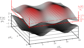
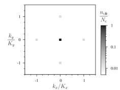
Figure 1: (a) Condensate density $n_{\rm c}(\bi{r})/n_{\rm c}$, perturbatively calculated via (8) and (9), in a square lattice potential $V(\bi{r})=V_{x}\cos(K_{x}x)+V_{y}\cos(K_{y}y)$ with $V_{x}=V_{y}=0.75gn_{c}$ and $K_{x}\xi=K_{y}\xi=1$. The condensate adapts a deformed configuation in the external potential by avoiding peaks and accumulating in wells. Due to the finite value of $K_{j}\xi$, the condensate profile is much smoother than the Thomas-Fermi profile $n_{\rm TF}(\bi{r})=n_{\rm c}-V(\bi{r})/g$, which falls to zero around $\bi{r}=0$ modulo the lattice period. (b) Corresponding condensate momentum distribution $n_{{\rm c}\bi{k}}/N_{c}$, Eq. (11), showing $1/16\approx 6\%$ of the total population in the $k$-components imprinted by the lattice.

When the external potential is weak, it is straightforward to solve the GP equation perturbatively to the desired order in powers of $V$ [10, 11]: $\Phi=\Phi^{(0)}+\Phi^{(1)}+\Phi^{(2)}+\dots$. In the following we work at fixed average condensate density $n_{\rm c}=L^{-d}\int\rmd^{d}r|\Phi(\bi{r})|^{2}$ and adjust the chemical potential accordingly [8]. In momentum representation, the homogeneous condensate $\Phi^{(0)}{k}=N_{\rm c}^{1/2}\delta_{\bi{k},0}$ receives the lowest-order deformations

$$\Phi{k}^{(1)} =-N_{\rm c}^{1/2}\tilde{V}{k},$$ (8)

$$\Phi^{(2)}{k} =\frac{N_{\rm c}^{1/2}}{2gn_{\rm c}+\epsilon^{0}_{k}}\sum{q}\tilde{V}_{\bi{k}-\bi{q}}\tilde{V}_{\bi{q}}\left[(1-\delta_{\bi{k}0})\epsilon^{0}_{q}-gn_{\rm c}\right].$$ (9)

The set of small parameters of this expansion are the reduced matrix elements

$$\tilde{V}{k}=\frac{1-\delta_{\bi{k},0}}{\epsilon^{0}_{k}+2gn_{\rm c}}V{k},$$ (10)

with $V{k}=L^{-d}\int\rmd^{d}r\rme^{-\rmi\bi{k}\cdot\bi{r}}V(\bi{r})$ the bare potential matrix element, $\epsilon^{0}_{k}=\hbar^{2}k^{2}/2m$ the bare kinetic energy, and $gn_{\rm c}=\mu^{(0)}$ the chemical potential in absence of the external potential. The condensate deformation follows the external potential only for $\epsilon^{0}_{k}\ll gn_{\rm c}$, or equivalently for wave vectors $k\xi\ll 1$ in terms of the healing length $\xi=\hbar/\sqrt{2mgn_{\rm c}}$. Consequently, the condensate momentum distribution up to order $V^{2}$ becomes

$$n_{{\rm c}\bi{k}}=|\Phi{k}|^{2}=N_{\rm c}\left[(1-V_{2})\delta_{\bi{k}0}+|\tilde{V}{k}|^{2}\right].$$ (11)

Most particles in this distribution still have zero momentum, but a small fraction

$$V_{2}\equiv\sum{k}|\tilde{V}{k}|^{2}\ll 1,$$ (12)

of them have been promoted to finite momenta by the weak external potential.

As an illustration, Fig. 1 shows the condensate density $n_{c}(\bi{r})$ and its momentum distribution $n_{\mathrm{c}\bi{k}}$, Eq. (11), in presence of a simple square lattice potential whose parameters are such that $V_{2}=1/16=6.25\%$. The external potential deforms the condensate, which tends to avoid potential peaks and accumulates in potential wells. The deformation is periodic in real space, Fig. 1(a). In $k$-space, the lattice shifts some population to the lattice momenta, Fig. 1(b). To higher order in the external potential, also higher-order components would become visible in the momentum distribution (cf. Fig. 2 in [12]).

2.3 Condensate deformation does not reduce mean-field condensate fraction

Condensate deformation is clearly a mean-field effect. The condensed part of the OBDM follows by inserting (11) into (5):

$$\rho_{\rm c}(\bi{s})=n_{\rm c}(1-V_{2})+n_{\rm c}\sum{k}\rme^{\rmi\bi{k}\cdot\bi{s}}|\tilde{V}{k}|^{2}.$$ (13)

By construction, $\rho_{\rm c}(0)=n_{\rm c}$ is the total density of condensed particles, which is kept fixed by adjusting the chemical potential. Consequently, constant potential offsets have no effect, and thus $\tilde{V}_{0}=0$ as implied by (10). Since $\tilde{V}_{0}=0$, one could be tempted to think that the fluctuating part in (13) tends to zero in the limit $s\to\infty$, which would imply that it does not contribute to the off-diagonal long-range order. However, this reasoning is erroneous, as becomes quite evident in the case of a general lattice potential

$$V(\bi{r})=\sum_{j=1}^{d}V_{j}\cos(\bi{K}_{j}\cdot\bi{r}).$$ (14)

By consequence of the lattice periodicity, also the OBDM deformation is periodic in $\bi{s}$,

$$\sum{k}\rme^{\rmi\bi{k}\cdot\bi{s}}|\tilde{V}{k}|^{2}=\frac{1}{2}\sum_{j=1}^{d}\tilde{V}_{j}^{2}\cos(\bi{K}_{j}\cdot\bi{s}),$$ (15)

with finite amplitudes $\tilde{V}_{j}=V_{j}/(\epsilon^{0}_{K_{j}}+2gn_{\rm c})$. But a periodic deformation cannot be bounded by a function $\gamma(s)$ that tends to zero, and so it is the full momentum distribution (9) that describes the condensate, in agreement with the Penrose-Onsager criterion. Indeed, the (wrong) conclusion that only part of the field $\Phi(\bi{r})$ constitutes the condensate would contradict the mean-field ansatz used to calculate it in the first place.

If one performs additional configuration averages, then one accesses no longer the full condensate fraction, but only its $\bi{k}=0$ component. As an example, consider the 2D lattice potential (14) of figure 1, and compute the angle-averaged OBDM $\overline{\rho}(s)=(2\pi)^{-1}\int\rmd\theta\rho(\bi{s})$ [5]. The inhomogeneous mean-field contribution (15) then averages to $\frac{1}{2}\sum_{j}\tilde{V}_{j}^{2}J_{0}(K_{j}s)$, with $J_{0}(.)$ the Bessel function. This function indeed goes to zero as $s\to\infty$ and thus yields, by construction, the translation-invariant component as a result. But working with an configuration-averaged OBDM does not prove that the zero-momentum component is a good indicator for BEC, since the argument would be circular. Within mean-field theory, the condensate fraction is unity, regardless of the specific form of the condensate mode $\Phi(\bi{r})$.

The same argument applies whenever an ensemble-average over a random potential distribution is performed. In fact, the supposed disorder-depleted density calculated in references [13, 14] really is the averaged condensate deformation $n_{c}\overline{V_{2}}$ that follows from (12) for a white-noise disorder potential.

Summarizing the mean-field discussion, we reiterate that Bose-Einstein condensates form in many different spatial shapes and with different momentum distributions, determined by the competition of kinetic, interaction, and potential energy. In a trap or any spatially inhomogeneous potential, the zero-momentum eigenstate relevant to free space has no reason to determine the condensation into a single-particle orbital. In short, the population of momentum $\bi{k}=0$ is not a good indicator for BEC in inhomogeneous systems.

As a consequence, the population of momenta $\bi{k}\neq 0$ does not measure the depletion of inhomogeneous condensates, contrary to what has been suggested, unfortunately, in the groundbreaking work of Huang and Meng [13], followed in this respect by numerous others [15, 14, 16, 17, 18, 19, 20, 21]. Within the Huang–Meng approximation scheme, one cannot calculate the condensate depletion induced by the external potential; this is achieved, for the first time to our knowledge, in Sec. 4 below. To this end, we require a theory for the fluctuations of inhomogeneous condensates.

3 Momentum distribution of quantum fluctuations

In this section, the momentum distribution $\delta n{k}$ of fluctuations, as defined by (6), is determined via Bogoliubov theory as a function of the external potential. For a weak potential, a perturbative, but fully analytical, expression is obtained.

3.1 Bogoliubov excitations of an inhomogeneous condensate

Fluctuations around the inhomogeneous ground state $\Phi(\bi{r})$ are best described using the density-phase representation: $\delta\hat{\Psi}(\bi{r})=\exp\{\rmi\delta\hat{\varphi}(\bi{r})\}[\Phi(\bi{r})^{2}+\delta\hat{n}(\bi{r})]^{1/2}-\Phi(\bi{r})$ develops as

$$\delta\hat{\Psi}(\bi{r})=\frac{1}{2n_{\rm c}}\check{\Phi}(\bi{r})\delta\hat{n}(\bi{r})+\rmi\Phi(\bi{r})\delta\hat{\varphi}(\bi{r})+\dots$$ (16)

Here, the inverse condensate amplitude $\check{\Phi}(\bi{r})=n_{\rm c}/\Phi(\bi{r})$ is well defined because weak external potentials do not fragment the condensate. Likewise, highly excited states such as vortices are not considered, and so $\Phi(\bi{r})>0$ holds everywhere.

Fluctuations define Bogoliubov quasi-particles, or “bogolons”. Mathematically, these are obtained by the canonical transformation [14]

$$\hat{\gamma}_{\bi{p}}=\delta\hat{n}{p}/(2a_{p}n_{\rm c}^{1/2})+\rmi a_{p}n_{\rm c}^{1/2}\delta\hat{\varphi}{p}.$$ (17)

Here, $a_{p}=(\epsilon^{0}_{p}/\epsilon_{p})^{1/2}$ for all $\bi{p}\neq 0$ is the traditional Bogoliubov transformation parameter, given by the ratio of free-particle dispersion $\epsilon^{0}_{p}=\hbar^{2}p^{2}/2m$ to the Bogoliubov dispersion $\epsilon_{p}=[\epsilon^{0}_{p}(\epsilon^{0}_{p}+2gn_{\rm c})]^{1/2}$. For the zero mode, it is appropriate to define $a_{0}=1$, as discussed in A. Importantly, the fluctuations $\delta\hat{n}{p}$ and $\delta\hat{\varphi}{p}$ are the Fourier components of density and phase deviations away from the deformed mean-field ground state $\Phi(\bi{r})$—and not from the homogeneous background $n_{\rm c}^{1/2}$ since then the deformation effect of the potential would be missed. By consequence of (17), the fluctuation (16) is expressed via bogolons as

$$\delta\hat{\Psi}{k}=\sum{p}\left(u_{\bi{k}\bi{p}}\hat{\gamma}_{\bi{p}}-v_{\bi{k}\bi{p}}\hat{\gamma}^{\dagger}_{-\bi{p}}\right),$$ (18)

where the inhomogeneous Bogoliubov transformation matrices

$$u_{\bi{k}\bi{p}} =\frac{1}{2\sqrt{N_{\rm c}}}\left[a_{p}^{-1}\Phi_{\bi{k}-\bi{p}}+a_{p}\check{\Phi}_{\bi{k}-\bi{p}}\right],$$ (19)

$$v_{\bi{k}\bi{p}} =\frac{1}{2\sqrt{N_{\rm c}}}\left[a_{p}^{-1}\Phi_{\bi{k}-\bi{p}}-a_{p}\check{\Phi}_{\bi{k}-\bi{p}}\right],$$ (20)

contain the Fourier coefficients of the condensate amplitude, $\Phi{k}=L^{-d/2}\int\rmd^{d}r\rme^{-\rmi\bi{k}\cdot\bi{r}}\Phi(\bi{r})$, and its inverse, $\check{\Phi}{k}=[n_{\rm c}/\Phi]{k}$. Some useful properties of this transformation to Bogoliubov quasiparticles are discussed in A.

Inserting (18) and its Hermitian conjugate into $\delta n{k}=\left\langle\smash{\delta\hat{\Psi}^{\dagger}{k}\delta\hat{\Psi}{k}}\right\rangle$ brings the fluctuation momentum distribution in the form

$$\delta n{k}=\sum_{\bi{p},\bi{p}^{\prime}}\left\{\delta_{\bi{p}\bi{p}^{\prime}}|v_{\bi{k}\bi{p}}|^{2}+\left(u_{\bi{k}\bi{p}}^{*}u_{\bi{k}\bi{p}^{\prime}}+v_{\bi{k}\bi{p}}^{*}v_{\bi{k}\bi{p}^{\prime}}\right)\left\langle\smash{\hat{\gamma}^{\dagger}_{\bi{p}}\hat{\gamma}_{\bi{p}^{\prime}}}\right\rangle-(u_{\bi{k}\bi{p}}^{*}v_{\bi{k}\bi{p}^{\prime}}\left\langle\smash{\hat{\gamma}^{\dagger}_{\bi{p}}\hat{\gamma}^{\dagger}_{-\bi{p}^{\prime}}}\right\rangle+c.c.)\right\}.$$ (21)

This equation holds to arbitrary order in potential strength $V$, as long as expansion (16) is valid, namely for a non-vanishing condensate amplitude $\Phi(\bi{r})$ and negligible higher-order fluctuations. In order to compute the expectation values $\left\langle\smash{\hat{\gamma}^{\dagger}_{\bi{p}}\hat{\gamma}_{\bi{p}^{\prime}}}\right\rangle$ and $\left\langle\smash{\hat{\gamma}^{\dagger}_{\bi{p}}\hat{\gamma}^{\dagger}_{-\bi{p}^{\prime}}}\right\rangle$, we need to specify the Hamiltonian of inhomogeneous Bogoliubov fluctuations.

3.2 Inhomogeneous Bogoliubov Hamiltonian

The quadratic Hamiltonian for the Bogoliubov excitations of an inhomogeneous Bose gas was derived in [8, 22] by a saddle-point expansion of the many-body Hamiltonian around the deformed ground-state solution $\Phi(\bi{r})$:

$$\hat{H}=\sum_{\bi{k}}\epsilon_{k}\hat{\Gamma}_{\bi{k}}^{\dagger}\hat{\Gamma}_{\bi{k}}+\sum_{\bi{k},\bi{k}^{\prime}}\hat{\Gamma}^{\dagger}_{\bi{k}}\mathcal{V}_{\bi{k}\bi{k}^{\prime}}\hat{\Gamma}_{\bi{k}^{\prime}}.$$ (22)

The Bogoliubov-Nambu (BN) pseudo spinor $\hat{\Gamma}_{\bi{k}}^{\dagger}=(\hat{\gamma}^{\dagger}_{\bi{k}},\hat{\gamma}_{-\bi{k}})/\sqrt{2}$ allows for a rather compact notation. The only approximation in the derivation of the Hamiltonian is the neglect of third and fourth order terms in the fluctuations. In contrast, (22) is still exact in the external potential strength and has the structure $\hat{H}=\hat{H}^{(0)}+\hat{H}^{(V)}$. The price to be paid for spatial inhomogeneity is the appearance of the effective scattering vertex

$$\mathcal{V}_{\bi{k}\bi{k}^{\prime}}=\left(\begin{array}[]{cc}W_{\bi{k}\bi{k}^{\prime}}&Y_{\bi{k}\bi{k}^{\prime}}\\ Y_{\bi{k}\bi{k}^{\prime}}&W_{\bi{k}\bi{k}^{\prime}}\end{array}\right).$$ (23)

Its matrix elements,

$$W_{\bi{k}\bi{k}^{\prime}} =\frac{1}{4}\left[a_{k}a_{k^{\prime}}R_{\bi{k}\bi{k}^{\prime}}+a_{k}^{-1}a_{k^{\prime}}^{-1}S_{\bi{k}\bi{k}^{\prime}}\right],$$ (24)

$$Y_{\bi{k}\bi{k}^{\prime}} =\frac{1}{4}\left[a_{k}a_{k^{\prime}}R_{\bi{k}\bi{k}^{\prime}}-a_{k}^{-1}a_{k^{\prime}}^{-1}S_{\bi{k}\bi{k}^{\prime}}\right],$$ (25)

are entirely determined by mean-field amplitudes $\Phi{k}$ and $\check{\Phi}{k}$ via

$$S_{\bi{k}\bi{k}^{\prime}} =\frac{2g}{L^{d}}\xi^{2}\bi{k}\cdot\bi{k}^{\prime}(1-\delta_{\bi{k}\bi{k}^{\prime}})\sum{p}\Phi_{\bi{k}-\bi{p}}\Phi_{\bi{p}-\bi{k}^{\prime}},$$ (26)

$$R_{\bi{k}\bi{k}^{\prime}} =\frac{2g}{L^{d}}\xi^{2}\sum{p}\left[\bi{k}\cdot\bi{k}^{\prime}+(\bi{k}+\bi{k}^{\prime}-2\bi{p})^{2}\right]\check{\Phi}_{\bi{k}-\bi{p}}\check{\Phi}_{\bi{p}-\bi{k}^{\prime}}-2\epsilon^{0}_{k}\delta_{\bi{k}\bi{k}^{\prime}}.$$ (27)

Here, we have dropped the superscripts $S^{(V)}$ and $R^{(V)}$ used in [8].

3.3 Bogolon populations

It is in principle possible to diagonalize the Hamiltonian (22) numerically, for each realization of the external potential, after having solved the nonlinear GP equation (7). However, for the purpose of analytical calculations in weak external potentials, a more economic strategy is to calculate the bogolon populations required in (21) perturbatively. We assume an equilibrium state at finite temperature $T$. The normal expectation value can be expressed via the single-quasiparticle Matsubara-Green (MG) function:

$$\left\langle\smash{\hat{\gamma}^{\dagger}_{\bi{p}^{\prime}}\hat{\gamma}_{\bi{p}}}\right\rangle=-\lim_{\tau\to 0^{-}}G_{\bi{p}\bi{p}^{\prime}}(\tau)=-\frac{1}{\beta}\sum_{n\in\mathbbm{Z}}G_{\bi{p}\bi{p}^{\prime}}(i\omega_{n})$$ (28)

where $\omega_{n}=2\pi n/\beta$ are the bosonic Matsubara frequencies related to the inverse temperature $\beta=1/k_{\mathrm{B}}T$. Similarly, the anomalous expectation value

$$\left\langle\smash{\hat{\gamma}^{\dagger}_{\bi{p}^{\prime}}\hat{\gamma}^{\dagger}_{-\bi{p}}}\right\rangle=-\frac{1}{\beta}\sum_{n\in\mathbbm{Z}}F_{\bi{p}\bi{p}^{\prime}}(i\omega_{n})$$ (29)

is expressed in terms of the anomalous MG function $F(z)$. Together, the normal and anomalous MG function enter the Nambu-MG matrix $\mathcal{G}=\footnotesize\left(\begin{array}[]{cc}G&F^{\dagger}\\ F&G^{\dagger}\end{array}\right)$ which expands as $\mathcal{G}=\mathcal{G}_{0}+\mathcal{G}_{0}\mathcal{V}\mathcal{G}_{0}+\mathcal{G}_{0}\mathcal{V}\mathcal{G}_{0}\mathcal{V}\mathcal{G}_{0}+\dots$ The free propagator is diagonal in Nambu space and momentum representation, $\mathcal{G}_{0\bi{p}}(i\omega_{n})=\mathrm{diag}(G_{0\bi{p}}(i\omega_{n}),G_{0\bi{p}}(-i\omega_{n}))$ with $G_{0\bi{p}}(z)=[z-\epsilon_{p}]^{-1}$. Matsubara sums like (28) and (29) are carried out using textbook recipes such as (11.58) in [23]; each simple pole with energy $\epsilon_{p}$ contributes one Bose-Einstein occupation number

$$\nu:=\nu(\beta\epsilon_{p})=[\exp(\beta\epsilon_{p})-1]^{-1}.$$ (30)

The expectation values (28), (29) are then straightforward to calculate. For brevity, we present here only the diagonal result for $\bi{p}^{\prime}=\bi{p}$, i.e. the bogolon population $\nu{p}\equiv\left\langle\smash{\hat{\gamma}^{\dagger}_{\bi{p}}\hat{\gamma}_{\bi{p}}}\right\rangle$, up to order $\mathcal{V}^{2}$:

$$\nu{p}=\nu+\frac{\partial\nu}{\partial\epsilon}W_{\bi{p}\bi{p}}+\sum_{\bi{p}^{\prime}} \left\{\frac{1}{\epsilon-\epsilon^{\prime}}\left(\frac{\partial\nu}{\partial\epsilon}-\frac{\nu^{\prime}-\nu}{\epsilon^{\prime}-\epsilon}\right)W_{\bi{p}\bi{p}^{\prime}}W_{\bi{p}^{\prime}\bi{p}}\right.$$ (31)

$$-\left.\frac{1}{\epsilon+\epsilon^{\prime}}\left(\frac{\partial\nu}{\partial\epsilon}-\frac{1+\nu^{\prime}+\nu}{\epsilon^{\prime}+\epsilon}\right)Y_{\bi{p}\bi{p}^{\prime}}Y_{\bi{p}^{\prime}\bi{p}}\right\}.$$

Here the short-hand notations $\epsilon=\epsilon_{p}$, $\epsilon^{\prime}=\epsilon_{p^{\prime}}$, and $\nu^{\prime}=\nu(\beta\epsilon^{\prime})$ are used. At temperature $T=0$ when all occupation numbers and their derivatives vanish, there is only a single finite contribution to the normal bogolon population due to the external potential, to order $\mathcal{V}^{2}$:

$$\nu_{\bi{p}}=\sum_{\bi{p}^{\prime}}\frac{1}{(\epsilon+\epsilon^{\prime})^{2}}Y_{\bi{p}\bi{p}^{\prime}}Y_{\bi{p}^{\prime}\bi{p}}.$$ (32)

The bogolon quasi-particles are populated by the random potential even at zero temperature because the full Hamiltonian (22) is not diagonal in the basis that diagonalizes $H^{(0)}$.

Similarly, the anomalous population $\pi{p}=-\left\langle\smash{\hat{\gamma}^{\dagger}_{\bi{p}}\hat{\gamma}^{\dagger}_{-\bi{p}}}\right\rangle$ reads, to order $\mathcal{V}^{2}$,

$$\pi{p}=\frac{1+2\nu}{2\epsilon}Y_{\bi{p}\bi{p}}-\frac{1}{\epsilon}\sum_{\bi{p}^{\prime}}\frac{\epsilon-\epsilon^{\prime}+2(\epsilon\nu^{\prime}-\epsilon^{\prime}\nu)}{(\epsilon-\epsilon^{\prime})(\epsilon+\epsilon^{\prime})}Y_{\bi{p}\bi{p}^{\prime}}W_{\bi{p}^{\prime}\bi{p}}.$$ (33)

At $T=0$, the result simplifies slightly:

$$\pi_{\bi{p}}=\frac{1}{2\epsilon}Y_{\bi{p}\bi{p}}-\frac{1}{\epsilon}\sum_{\bi{p}^{\prime}}\frac{1}{\epsilon+\epsilon^{\prime}}Y_{\bi{p}\bi{p}^{\prime}}W_{\bi{p}^{\prime}\bi{p}}.$$ (34)

With this, everything is in place to calculate the full momentum distribution (21), or equivalently the OBDM (5). In the following, we pursue a fully analytical calculation by a perturbative expansion up to order $V^{2}$ in the bare external potential. In the upcoming section 3.4 the Bogoliubov transformation matrices (19) and (20) are determined together with the scattering matrix elements (24) and (25). In Sec. 3.5 the results are collected into a compact expression for the momentum distribution.

3.4 Weak-potential expansion

The perturbation expansion (8)–(9) of the condensate amplitude $\Phi{k}$ in powers of $V$ implies a similar expansion for the Bogoliubov transformation matrices (19) and (20):

$$u_{\bi{k}\bi{p}}=u_{\bi{k}\bi{p}}^{(0)}+u_{\bi{k}\bi{p}}^{(1)}+u_{\bi{k}\bi{p}}^{(2)}+\dots,$$ (35)

$$v_{\bi{k}\bi{p}}=v_{\bi{k}\bi{p}}^{(0)}+v_{\bi{k}\bi{p}}^{(1)}+v_{\bi{k}\bi{p}}^{(2)}+\dots$$ (36)

To zeroth order in the external potential, the transformation matrices are diagonal in momentum, as required by translation invariance, and the traditional Bogoliubov amplitudes are recovered:

$$u_{\bi{k}\bi{p}}^{(0)}=\frac{1}{2}(a_{p}^{-1}+a_{p})\delta_{\bi{k}\bi{p}}\equiv u_{p}\delta_{\bi{k}\bi{p}},$$ (37)

$$v_{\bi{k}\bi{p}}^{(0)}=\frac{1}{2}(a_{p}^{-1}-a_{p})\delta_{\bi{k}\bi{p}}\equiv v_{p}\delta_{\bi{k}\bi{p}}.$$ (38)

To first order, the matrix elements are proportional to the potential matrix element (10):

$$u_{\bi{k}\bi{p}}^{(1)}=-v_{p}\tilde{V}_{\bi{k}-\bi{p}},\qquad v_{\bi{k}\bi{p}}^{(1)}=-u_{p}\tilde{V}_{\bi{k}-\bi{p}}.$$ (39)

For the second-order matrices, only the diagonal matrix elements will be required:

$$u_{\bi{k}\bi{k}}^{(2)}=\frac{u_{k}-2v_{k}}{2}V_{2},\qquad v_{\bi{k}\bi{k}}^{(2)}=\frac{v_{k}-2u_{k}}{2}V_{2},$$ (40)

where $V_{2}$ of Eq. (12) is second order in $V$.

As spelled out in [8], also the BN scattering potential (23) admits the expansion $\mathcal{V}=\mathcal{V}^{(1)}+\mathcal{V}^{(2)}+\dots$. Also here, the first-order scattering amplitudes

$$W^{(1)}_{\bi{k}\bi{p}}=gn_{\rm c}\tilde{w}^{(1)}_{\bi{k}\bi{p}}\tilde{V}_{\bi{k}-\bi{p}},\qquad Y^{(1)}_{\bi{k}\bi{p}}=gn_{\rm c}\tilde{y}^{(1)}_{\bi{k}\bi{p}}\tilde{V}_{\bi{k}-\bi{p}}$$ (41)

are proportional to (10), with

$$\tilde{w}^{(1)}_{\bi{k}\bi{p}} =\xi^{2}\left[a_{k}a_{p}(k^{2}+p^{2}-\bi{k}\cdot\bi{p})-{a_{k}^{-1}a_{p}^{-1}}\bi{k}\cdot\bi{p}\right]$$ (42)

$$=\xi^{2}\left[(u_{k}-v_{k})(u_{p}-v_{p})(k^{2}+p^{2})-2(u_{k}u_{p}+v_{k}v_{p})\bi{k}\cdot\bi{p}\right],$$

$$\tilde{y}^{(1)}_{\bi{k}\bi{p}} =\xi^{2}\left[a_{k}a_{p}(k^{2}+p^{2}-\bi{k}\cdot\bi{p})+a_{k}^{-1}a_{p}^{-1}\bi{k}\cdot\bi{p}\right]$$ (43)

$$=\xi^{2}\left[(u_{k}-v_{k})(u_{p}-v_{p})(k^{2}+p^{2})+2(u_{k}v_{p}+v_{k}u_{p})\bi{k}\cdot\bi{p}\right].$$

Second-order scattering amplitudes are later only needed for $\bi{k}=\bi{p}$:

$$W^{(2)}_{\bi{k}\bi{k}}=Y^{(2)}_{\bi{k}\bi{k}}=gn_{\rm c}\sum_{\bi{p}}\tilde{y}^{(2)}_{\bi{k}\bi{p}}|\tilde{V}_{\bi{k}-\bi{p}}|^{2}$$ (44)

with

$$\tilde{y}^{(2)}_{\bi{k}\bi{p}}=2a_{k}^{2}\xi^{2}[k^{2}+(\bi{k}-\bi{p})^{2}].$$ (45)

3.5 Momentum distribution

Collecting all results up to order $V^{2}$, the single-particle fluctuation momentum distribution (21) reads

$$\delta n{k}=\left\langle\smash{\delta\hat{\Psi}^{\dagger}{k}\delta\hat{\Psi}{k}}\right\rangle=\delta n{k}^{(0)}+\delta n{k}^{(2)},$$ (46)

where the superscript indicates the order in the external potential strength $V$. To zeroth order, i.e. for the homogeneous system, we recover the well known zero-temperature momentum distribution [7]

$$\delta n{k}^{(0)}=v_{k}^{2}=\frac{(a_{k}-a_{k}^{-1})^{2}}{4}=\frac{(\epsilon_{k}-\epsilon^{0}_{k})^{2}}{4\epsilon_{k}\epsilon^{0}_{k}}=\frac{1+(k\xi)^{2}}{2k\xi\sqrt{2+(k\xi)^{2}}}-\frac{1}{2}$$ (47)

as a consequence of the two-body contact interaction. The first-order term vanishes by momentum conservation, $\delta n{k}^{(1)}=0$. The external potential induces the second-order shift

$$\delta n{k}^{(2)}=\sum{p}\tilde{M}^{(2)}_{\bi{k}\bi{p}}|\tilde{V}_{\bi{k}-\bi{p}}|^{2},$$ (48)

whose kernel is defined in terms of (42), (43), and (45):

$$\tilde{M}^{(2)}_{\bi{k}\bi{p}} =(v_{k}^{2}-2u_{k}v_{k}+u_{p}^{2})-2(u_{k}u_{p}+v_{k}v_{p})\frac{gn_{\rm c}\tilde{y}^{(1)}_{\bi{k}\bi{p}}}{\epsilon_{k}+\epsilon_{p}}$$ (49)

$$+(u_{k}^{2}+v_{k}^{2})\frac{(gn_{\rm c}\tilde{y}^{(1)}_{\bi{k}\bi{p}})^{2}}{(\epsilon_{k}+\epsilon_{p})^{2}}+\frac{gn_{\rm c}u_{k}v_{k}}{\epsilon_{k}}\left\{\tilde{y}^{(2)}_{\bi{k}\bi{p}}-\frac{2gn_{\rm c}}{\epsilon_{k}+\epsilon_{p}}\tilde{y}^{(1)}_{\bi{k}\bi{p}}\tilde{w}^{(1)}_{\bi{k}\bi{p}}\right\}.$$

This expression, together with the preceding general form (21), constitutes the main result of this calculation. From here on, we explore its consequences by studying two generic examples of external potentials: a weak lattice potential on the one hand, and a random potential on the other.

3.5.1 Lattice potential –

A pure lattice potential like (14) has only the Fourier components $V{k}=\frac{1}{2}\sum_{j=1}^{d}V_{j}\left(\delta_{\bi{k},\bi{K}_{j}}+\delta_{\bi{k},-\bi{K}_{j}}\right)$, such that

$$|V{k}|^{2}=\frac{1}{4}\sum_{j=1}^{d}V_{j}^{2}\left(\delta_{\bi{k},\bi{K}_{j}}+\delta_{\bi{k},-\bi{K}_{j}}\right).$$ (50)

Thus, the momentum distribution shift (48) is given by

$$\delta n{k}^{(2)}=\frac{1}{4}\sum_{j=1}^{d}\frac{(V_{j}/gn_{\rm c})^{2}}{[2+(K_{j}\xi)^{2}]^{2}}\left(\tilde{M}^{(2)}_{\bi{k}\,\bi{k}+\bi{K}_{j}}+\tilde{M}^{(2)}_{\bi{k}\,\bi{k}-\bi{K}_{j}}\right).$$ (51)

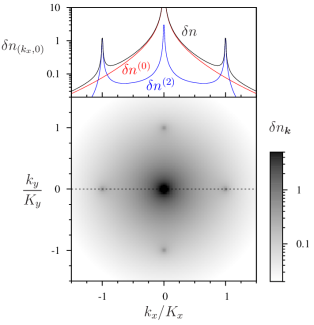
Figure 2: Zero-temperature momentum distribution $\delta n{k}$ of quantum fluctuations, Eq. (46), in the square lattice potential of Fig. 1. The upper panel shows a cut along $k_{y}=0$. The main contribution stems from the isotropic background $\delta n^{(0)}{k}$, Eq. (47). The potential-induced distribution $\delta n^{(2)}{k}$, Eq. (51), reflects the lattice structure.

Figure 2 shows the momentum distribution (46) in the square lattice potential of Fig. 1. The top panel shows a cut through the distribution at $k_{y}=0$, together with the separate contributions of the homogeneous and potential-induced distribution. Compared to the mean-field figure 1, the quantum fluctuations broaden the momentum distribution substantially.

In formula (51), the product $K_{j}\xi$ compares the characteristic length scale of the potential, $K_{j}^{-1}$, with the condensate healing length $\xi$. For not-too-low densities and typical interaction strengths achievable with ultracold atoms, one easily reaches $K_{j}\xi\ll 1$, known as the Thomas-Fermi (TF) regime. The healing length is the characteristic scale also for the entire kernel (49). In the deep TF regime $K_{j}\xi\to 0$, and for finite momenta $k>K_{j}$, this complicated kernel can be approximated by the diagonal term $\tilde{M}_{\bi{k}\bi{k}}^{(2)}=[(k\xi)^{2}-1]/\{k\xi[2+(k\xi)^{2}]^{5/2}\}$. The potential-induced change of momentum distribution then takes the simple isotropic form

$$\delta n_{\bi{k}\mathrm{TF}}^{(2)}=\frac{v^{2}}{4}\frac{(k\xi)^{2}-1}{k\xi[2+(k\xi)^{2}]^{5/2}}.$$ (52)

Here, $v^{2}=\frac{1}{2}\sum_{j}(V_{j}/gn_{\rm c})^{2}$ measures the potential variance in units of the mean-field interaction energy. In the TF regime (52), the external potential is found to shift population from low momenta $k\xi<1$ to high momenta $k\xi>1$, and this independently of the detailed form of the potential.

3.5.2 Random potential –

A random potential can be seen as a superposition of many lattices with a random distribution of Fourier components $V{k}$, specified by the ensemble averages $\overline{V{k}}$, $\overline{V{k}V{p}}$, etc. Here, we assume without loss of generality that the potential is centred, $\overline{V(\bi{r})}=0$ or $V_{0}=0$. All we need at order $V^{2}$ then is the pair correlator

$$\overline{V{q}V_{-\bi{q}^{\prime}}}=L^{-d}\delta_{\bi{q}\bi{q}^{\prime}}V^{2}\sigma^{d}C_{d}(\bi{q}\sigma).$$ (53)

The dimensionless function $C_{d}(\bi{q}\sigma)$ characterizes the potential correlation on the length scale $\sigma$; the normalization is chosen such that $(\sigma/L)^{d}\sum{q}C_{d}(\bi{q}\sigma)=1$ in the thermodynamic limit. Using (53), the ensemble-averaged change of the single-particle momentum distribution (48) takes the form

$$\overline{\delta n}^{(2)}_{\bi{k}}=v^{2}\frac{\sigma^{d}}{L^{d}}\sum{q}\tilde{M}^{(2)}_{\bi{k}\,\bi{k}-\bi{q}}\frac{C_{d}(\bi{q}\sigma)}{[2+(q\xi)^{2}]^{2}}$$ (54)

where $v^{2}=(V/gn_{\rm c})^{2}$ is the potential variance in units of mean-field interaction energy.

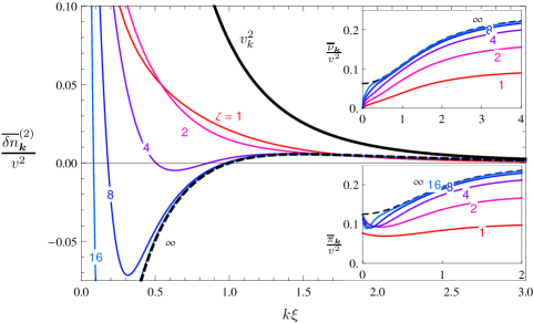
Figure 3: Quantum-fluctuation momentum distribution shift (54) induced by a 2D random potential of reduced variance $v^{2}=V^{2}/(gn_{\rm c})^{2}$ and Gaussian correlation, (55), for different values of the correlation length relative to the condensate healing length, $\zeta=\sigma/\xi$. For comparison, also the momentum distribution $\delta n^{(0)}_{k}=v_{k}^{2}$, Eq. (47), of the homogeneous fluctuations is shown. The insets show the normal and anomalous populations of Bogoliubov excitations, (56) and (57), respectively, also as function of $k\xi$. In the TF limit $\zeta\to\infty$, all distributions converge towards the universal expressions (52), (58), and (59), respectively, shown in dashed black.

Figure 3 shows the ensemble-averaged, isotropic, momentum distribution (54) that is induced by a random potential with Gaussian correlation

$$C_{d}(q\sigma)=(2\pi)^{d/2}\exp\{-q^{2}\sigma^{2}/2\}$$ (55)

in $d=2$ dimensions as function of $|\bi{k}|\xi$. Different curves correspond to different values of the correlation parameter $\zeta=\sigma/\xi$, namely the correlation length relative to the condensate healing length. Just as for the lattice, also here things simplify considerably in the TF regime $\sigma\gg\xi$ where the disorder correlation length is much longer than the condensate healing length. Then, the potential correlator tends to a $\delta$-distribution, and (54) reduces to (52), plotted in dashed black. Clearly, the momentum distribution of quantum fluctuations is given by the universal form (52) in any external potential that is sufficiently smooth to yield a Thomas-Fermi condensate profile.

The insets of Fig. 3 show the ensemble-averaged, normal and anomalous bogolon populations $\nu{k}=\left\langle\smash{\hat{\gamma}^{\dagger}_{\bi{k}}\hat{\gamma}_{\bi{k}}}\right\rangle$ and $\pi{k}=-\left\langle\smash{\hat{\gamma}^{\dagger}_{\bi{k}}\hat{\gamma}^{\dagger}_{-\bi{k}}}\right\rangle$ at zero temperature. These populations, (32) and (34), are given by

$$\overline{\nu}_{\bi{k}} =V^{2}\frac{\sigma^{d}}{L^{d}}\sum{q}\frac{(\tilde{y}^{(1)}_{\bi{k}\,\bi{k}-\bi{q}})^{2}}{(\epsilon_{\bi{k}}+\epsilon_{\bi{k}-\bi{q}})^{2}}\frac{C_{d}(\bi{q}\sigma)}{[2+(q\xi)^{2}]^{2}},$$ (56)

$$\overline{\pi}_{\bi{k}} =V^{2}\frac{\sigma^{d}}{L^{d}}\sum{q}\left\{\frac{\tilde{y}^{(2)}_{\bi{k}\,\bi{k}-\bi{q}}}{2gn_{\rm c}\epsilon_{\bi{k}}}-\frac{\tilde{y}^{(1)}_{\bi{k}\,\bi{k}-\bi{q}}\tilde{w}^{(1)}_{\bi{k}\,\bi{k}-\bi{q}}}{\epsilon_{\bi{k}}(\epsilon_{\bi{k}}+\epsilon_{\bi{k}-\bi{q}})}\right\}\frac{C_{d}(\bi{q}\sigma)}{[2+(q\xi)^{2}]^{2}},$$ (57)

in terms of the envelopes (42), (43), and (45). In the TF regime, they tend toward the universal limiting expressions (dashed black in the insets of Fig. 3)

$$\overline{\nu}_{\bi{k}\mathrm{TF}}=\frac{v^{2}}{4}\frac{[1+(k\xi)^{2}]^{2}}{[2+(k\xi)^{2}]^{2}},$$ (58)

$$\overline{\pi}_{\bi{k}\mathrm{TF}}=\frac{v^{2}}{4}\frac{2+4(k\xi)^{2}+(k\xi)^{4}}{[2+(k\xi)^{2}]^{2}},$$ (59)

and this independently of the potential details.

4 Quantum depletion of the condensate

The total particle density $\rho(0)=n=n_{\rm c}+\delta n$ is the sum of condensate density $n_{\rm c}$ and non-condensed density $\delta n$. The condensate fraction is $n_{\rm c}/n=1-\delta n/n$. Within Bogoliubov theory, the existence of a finite non-condensed fraction $\delta n/n$ at temperature $T=0$ is called “quantum depletion”, because it arises from quantum fluctuations around the mean-field approximation to the true condensate. From a many-body point of view, the non-condensed fraction is of course not more quantum than the condensed one, or perhaps even rather less. Here, we follow the established nomenclature and continue to speak of quantum depletion, at zero temperature, as opposed to the thermal depletion at finite temperature.

From definitions (5) and (6) it follows that the depleted density $\delta n=n-n_{\rm c}$ is the integral of the fluctuation momentum distribution,

$$\delta n=L^{-d}\sum{k}\delta n{k}.$$ (60)

4.1 Homogeneous system

Let us first recall the homogeneous case $V=0$ [7]. Since condensation occurs in the $\bi{k}=0$ mode, the depleted density simply contains all particles with finite momenta, and the zero-temperature momentum distribution (47) implies

$$\delta n^{(0)}=L^{-d}\sum_{\bi{k}\neq 0}v_{k}^{2}.$$ (61)

In $d=3$, Eq. (61) evaluates to the depleted density $\delta n^{(0)}=[6\sqrt{2}\pi^{2}\xi^{3}]^{-1}$ in the thermodynamic limit. Equivalently, the relative depletion reads $\delta n^{(0)}/n=8(na_{s}^{3})^{1/2}/3\pi^{1/2}$ because $g=4\pi\hbar^{2}a_{s}/m$ in terms of the s-wave scattering length $a_{s}$ and $\xi^{2}=\hbar^{2}/(2mgn)$ (to leading order, we can identify $n_{\rm c}\approx n$ in all perturbative results). The Bogoliubov ansatz is justified whenever the fractional depletion is small, $\delta n^{(0)}\ll n$ or equivalently $n\xi^{d}\gg 1$. This is the case whenever the so-called gas parameter $na_{s}^{3}$ is small, i.e., for low enough density or weak scattering.

In $d=2$, one finds $\delta n^{(0)}=[8\pi\xi^{2}]^{-1}$, which is also the result of diagrammatic theory for hard-core bosons [24]. The quantum depletion $\delta n^{(0)}/n$ is roughly independent of density, and requires weak scattering.

In $d=1$, the infrared $k^{-1}$-divergence of $v_{k}$ under the integral prevents the existence of a homogeneous 1D condensate. In small enough systems, however, and at very low temperature, phase fluctuations remain small, and quasi-condensates have all the attributes of a true condensate [25, 26, 27, 28, 29]. Presently, we are interested in the effect of an external potential on the homogeneous situation. So we resort to cutting off the 1D-integral at some value $\alpha=\xi k_{\mathrm{IR}}\ll 1$, with $k_{\mathrm{IR}}$ of the order of the inverse system size, and find $\delta n^{(0)}=(2\ln 2-2-\ln\alpha)/(2\sqrt{2}\pi\xi)$, up to order $\alpha$. Bogoliubov theory then is valid whenever $n\xi\gg 1$, i.e., requires high enough density in order for the mean-field picture to apply in the first place.

So in all relevant dimensionalities, there is a window of validity for Bogoliubov theory, and the depleted density can be written $\delta n^{(0)}=c_{d}\xi^{-d}$, with a $d$-dependent numerical constant $c_{d}$ of order unity or smaller.

4.2 Potential depletion

In an inhomogeneous system, the quantum depletion cannot be calculated by counting all particles with finite momentum, as argued in Sec. (2) above. Instead, the depleted density (60) is the integral of the fluctuation momentum distribution (21), which splits into two contributions: the quantum depletion of the homogeneous system plus the potential-induced depletion properly speaking. The external potential can change the condensate fraction because it modifies the local particle density. This change in particle density changes the local interaction energy, which in turn changes the depletion. Since the interacting system has a nonlinear response, even in a purely sinusoidal lattice potential the high-density regions will deplete more condensate than the low-density regions can gain back. At the end, the presence of the potential causes a net additional depletion of the condensate, an effect that we propose to call “potential depletion”.

To our knowledge, the potential depletion, beyond the mean-field deformation of the condensate, has never been calculated analytically. In approaches very similar to ours, Singh and Rokhsar [30] arrived at numerical results for the potential depletion; Lee and Gunn [31] estimated a different depletion. Within our inhomogeneous Bogoliubov theory, computing the potential depletion is straightforward: Using the perturbative result (48) in (60), we find for the potential-depleted density

$$\delta n^{(2)}=L^{-d}\sum_{\bi{k},\bi{q}}\tilde{M}^{(2)}_{\bi{k}\,\bi{k}-\bi{q}}|\tilde{V}{q}|^{2}=\frac{1}{\xi^{d}(gn_{\rm c})^{2}}\sum_{\bi{q}}M_{d}(q\xi)|V{q}|^{2}.$$ (62)

The sum over $\bi{k}$ can be carried out without touching the potential, whence the second equality, which defines the isotropic depletion kernel for the bare potential,

$$M_{d}(q\xi)=\frac{(\xi/L)^{d}}{[2+(q\xi)^{2}]^{2}}\sum{k}\tilde{M}^{(2)}_{\bi{k}\,\bi{k}-\bi{q}}.$$ (63)

Prefactors are chosen such that in the thermodynamic limit $M_{d}(q\xi)$ is a dimensionless function of $q\xi$ only.

4.2.1 Lattice potential –

For the lattice potential (50), the potential depletion (62) reads

$$\delta n^{(2)}=\frac{1}{2\xi^{d}(gn_{\rm c})^{2}}\sum_{j=1}^{d}V_{j}^{2}M_{d}(K_{j}\xi).$$ (64)

For the 2D lattice potential of Figs. 1 and 2, one finds $\delta n^{(2)}=M_{2}(K\xi)V^{2}/(\xi gn_{\rm c})^{2}\approx 0.141\,\delta n^{(0)}$; for these parameters, the potential depletion amounts to only 14% of the homogeneous depletion. These results hold for weak lattices. In much deeper lattices, a tight-binding description becomes more appropriate [32, 33, 34].

Let us furthermore check (64) against the QMC results of Astrakharchik and Krutitsky [5], who investigated two different interaction strengths in a square lattice, such that $K\xi=6.275$, and $K\xi=1.984$, respectively. For these values, (64) predicts a potential depletion of $\delta n^{(2)}=1.05\,\delta n^{(0)}$, and $0.35\,\delta n^{(0)}$, respectively. If one takes the QMC values for the homogeneous depletion as the reference, then the final condensate fraction should be $N_{0}/N=1-\delta n/n=0.98$ in the one case and $0.73$ in the other, which is in good agreement with the data [5], $N_{0}/N\approx 0.99$ and $0.7$, respectively. Incidentally, the Bogoliubov prediction for the clean depletion $\delta n^{(0)}/n$ does not agree so well with the data, which may be due to finite size effects or the slightly different interaction potential (hard-core bosons instead of s-wave scattering) used in the QMC approach.

4.2.2 Random potential –

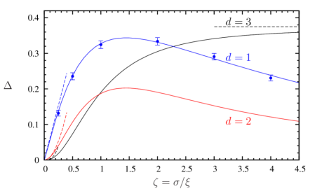
Figure 4: Disorder-induced quantum depletion (67), relative to the clean value and in units of disorder strength $v^{2}$, as function of the correlation ratio $\zeta=\sigma/\xi$ for the Gaussian correlation (55). The curve for $d=1$ depends weakly on the infrared cutoff $\alpha=\xi k_{\mathrm{IR}}$ that regularizes already the clean case; $\alpha=0.025$ in this plot. Data points are obtained by an exact numerical diagonalization of the Bogoliubov Hamiltonian (22) for $V=0.05gn_{\rm c}$, followed by an ensemble average over disorder. Error bars denote the estimated error for the average; the number $M$ of realizations is chosen for each point such that $ML/\sigma=4000$. Dashed: universal Thomas-Fermi limit $\Delta_{\mathrm{TF}}=3/8$ for very smooth disorder ($\zeta\to\infty$) in $d=3$. The curves for lower dimensions tend to $\Delta_{\mathrm{TF}}=0$ and $\Delta_{\mathrm{TF}}=-1/8$, in $d=2$ and $d=1$, respectively. Dotted: limiting behaviour for $\delta$-correlated disorder ($\zeta\ll 1$): $\Delta(\zeta)=\beta_{d}\zeta^{d}C_{d}(0)$ with $\beta_{1}\approx 0.245$ (for $\alpha=0.05$), $\beta_{2}\approx 0.135$, $\beta_{3}\approx 0.160$.

Using the momentum distribution (54) in (60), the quantum depletion (62) by a random potential with correlation (53) is found to be

$$\overline{\delta n}{}^{(2)}=\frac{V^{2}\sigma^{d}}{(gn_{\rm c})^{2}\xi^{d}L^{d}}\sum_{\bi{q}}M_{d}(q\xi)C_{d}(\bi{q}\sigma).$$ (65)

Scaled by the homogeneous depletion in the thermodynamic limit, this can be written as

$$\overline{\delta n}{}^{(2)}=v^{2}\delta n^{(0)}\Delta(\zeta)$$ (66)

where $v=V/(gn_{\rm c})$ and

$$\Delta(\zeta)=\frac{\zeta^{d}}{c_{d}}\int\frac{\rmd^{d}u}{(2\pi)^{d}}M_{d}(u)C_{d}(\bi{u}\zeta).$$ (67)

This relative potential depletion is found to be a function of the correlation ratio $\zeta=\sigma/\xi$. Only in $d=1$, it depends also very weakly on the cutoff $\alpha$ that regularizes already the clean depletion. The convergent integrals (66) require no additional ad-hoc cutoffs, neither infrared (since the excitations are orthogonal to the vacuum) nor ultraviolet (since potential correlations are included). Fig. 4 shows $\Delta(\zeta)$ for a Gaussian-correlated random potential (55) in dimensions $d=1,2,3$. Data points result from the numerical diagonalization of the Bogoliubov Hamiltonian (22) in a system of linear size $L$ such that $\alpha=\xi/L=0.05$, followed by an ensemble average over disorder. The exact shape of the curve depends on the correlation function, the general features, however, are rather robust.

The asymptotic behaviour of $\Delta(\zeta)$ for very small or very large correlation lengths is simple. In the $\delta$-correlated limit $\zeta\to 0$ of a white-noise potential, the generic scaling of (67) is $\Delta(\zeta)=\beta_{d}\zeta^{d}C_{d}(0)$ with $\beta_{d}=c_{d}^{-1}\int\frac{\rmd^{d}u}{(2\pi)^{d}}M_{d}(u)$. The numerical coefficients are $\beta_{1}\approx 0.245$ (weakly dependent on the cutoff $\alpha$), $\beta_{2}\approx 0.135$, $\beta_{3}\approx 0.160$. In this white-noise regime, the depletion depends on $\sigma^{d}C_{d}(0)$, and thus requires the existence of a microscopic correlation scale. In the opposite limit $\zeta\to\infty$ of the Thomas-Fermi regime, the result converges to a truly universal limit

$$\Delta_{\mathrm{TF}}=c_{d}^{-1}M_{d}(0)=\frac{1}{v^{2}\delta n^{(0)}}\int\frac{\rmd^{d}k}{(2\pi)^{d}}\overline{\delta n}^{(2)}_{\bi{k}\mathrm{TF}}$$ (68)

and evaluates, using (52), to $\Delta_{\mathrm{TF}}=3/8$ in $d=3$ and $\Delta_{\mathrm{TF}}=0$ in $d=2$. In 2 and 3 dimensions, the depletion is non-negative, as one would expect for a random potential that should broaden the momentum distribution overall. For $d=1$ the TF-limit evaluates to the negative value $\Delta_{\mathrm{TF}}=-1/8$ (in the limit of infinite system size). This would seem to imply that the random potential re-populates the condensate. But also in $d=1$ the depletion is positive for most values of $\zeta$, as shown in Fig. 4. The curve only crosses over to negative values for such a large value $\zeta=\sigma/\xi$ (depending on the cutoff $\alpha$), that the correlation length $\sigma$ has to be comparable to the system size, which is not the regime of present interest.

Interestingly, the TF limit for the potential depletion can also be derived by the local-density approximation (LDA) $n_{\mathrm{TF}}=n_{\rm c}-V(\bi{r})/g$ combined with the scaling $\delta n=c_{d}\xi^{-d}=c^{\prime}_{d}n_{\rm c}^{d/2}$ of the homogeneous depletion (Sec. 4.1):

$$\overline{\delta n_{\mathrm{TF}}}=c_{d}^{\prime}n_{c}^{d/2}\overline{[1-V(\bi{r})/gn_{\rm c}]^{d/2}}=\delta n^{(0)}\left[1+\frac{d(d-2)}{8}v^{2}+O(v^{3})\right]$$

and thus $\Delta_{\mathrm{TF}}=d(d-2)/8$, in agreement with the result of (68). This argument shows that in $d=2$ dimensions, the TF potential depletion is zero even non-perturbatively since $\overline{V}=0$ without loss of generality. This LDA reasoning works for the correction of the depletion, but not for the excitation dispersion relation, where genuine scattering effects determine corrections to the speed of sound and density of states [8, 35], and furthermore cause exponential localization [11, 36, 37].

Summarizing the results of this section, we conclude that the combined depletion due to interaction and external potential reads

$$\delta n=\delta n^{(0)}[1+v^{2}\Delta],$$ (69)

with $|\Delta|\ll 1$. Clearly, the potential depletion alone, $\delta n^{(2)}/n=(\delta n^{(0)}/n)v^{2}\Delta$, is at least a factor $\delta n^{(0)}/n\ll 1$ smaller than the mean-field condensate deformation (11), which is of order $v^{2}$. In hindsight, this result is rather plausible: the primary effect of the external potential is merely to deform the condensate. The potential depletion is a secondary effect, caused by enhanced interaction in the regions of higher density. We conclude that, as long as the original assumption of a non-zero condensate amplitude holds, our inhomogeneous Bogoliubov theory applies to Bose condensates in rather inhomogeneous potentials.

5 Summary

We have investigated the effect of external potentials on Bose-condensed gases using inhomogeneous Bogoliubov theory. The principal effect of an external potential is to deform the mean-field condensate. Secondly, the potential affects the momentum distribution of quantum fluctuations, for which we have obtained a general expression. Finally, we have calculated the quantum depletion induced by the external potential, or potential depletion for short. In detail, we have studied lattices and spatially correlated random potentials. The potential depletion turns out to be proportional to the homogeneous depletion, a fact that underscores the applicability of inhomogeneous Bogoliubov theory in weak to moderately strong potentials. Our analytical predictions are in agreement with a numerical diagonalization of the Bogoliubov Hamiltonian as well as with recent quantum Monte Carlo simulations [5]. The inhomogeneous Bogoliubov theory shown at work here is therefore proven capable of describing the excitations of weakly interacting condensates in external potentials, and from there ought to provide many of other static and dynamic properties.

Appendix A Transformation to Bogoliubov quasi-particles

The matrices $u_{\bi{k}\bi{p}}$ and $v_{\bi{k}\bi{p}}$ as defined by (19) and (20) are the Fourier components with wave vector $\bi{k}$ of the modes $u{p}(\bi{r})$ and $v{p}(\bi{r})$ defined in [8]. As explained there, the momentum index $\bi{p}$ can be used to label the modes even in the inhomogeneous setting. The transformation (18) preserves the canonical commutation relation, and thus guarantees $[\hat{\gamma}_{\bi{p}},\hat{\gamma}^{\dagger}_{\bi{p}^{\prime}}]=\delta_{\bi{p}\bi{p}^{\prime}}$ as well as $[\hat{\gamma}_{\bi{p}},\hat{\gamma}_{\bi{p}^{\prime}}]=0$, via the completeness relations

$$\sum{p}\left(u_{\bi{k}\bi{p}}u_{\bi{k}^{\prime}\bi{p}}^{*}-v_{\bi{k}\bi{p}}v_{\bi{k}^{\prime}\bi{p}}^{*}\right)=\delta_{\bi{k}\bi{k}^{\prime}},$$ (70)

$$\sum{p}\left(u_{\bi{k}\bi{p}}v_{\bi{k}^{\prime}\bi{p}}^{*}-v_{\bi{k}\bi{p}}u_{\bi{k}^{\prime}\bi{p}}^{*}\right)=0.$$ (71)

The non-symmetric matrices $u_{\bi{k}\bi{p}}\neq u_{\bi{p}\bi{k}}$ and $v_{\bi{k}\bi{p}}\neq v_{\bi{p}\bi{k}}$ also satisfy the biorthogonality

$$\sum{k}(u_{\bi{k}\bi{p}}u_{\bi{k}\bi{p}^{\prime}}^{*}-v_{\bi{k}\bi{p}}v_{\bi{k}\bi{p}^{\prime}}^{*})=\delta_{\bi{p}\bi{p}^{\prime}},$$ (72)

$$\sum{k}(u_{\bi{k}\bi{p}}v_{\bi{k}\bi{p}^{\prime}}^{*}-v_{\bi{k}\bi{p}}u_{\bi{k}\bi{p}^{\prime}}^{*})=0.$$ (73)

The zero mode deserves special attention because $a_{p}=(\epsilon^{0}_{p}/\epsilon_{p})^{1/2}$ diverges as $p^{-1}$ when $p\to 0$. In this range, elementary excitations are essentially phase fluctuations. Setting $a_{0}=1$, one finds that the Bogoliubov excitation

$$\hat{\gamma}_{0}=\delta\hat{n}_{0}/(2n_{\rm c}^{1/2})+\rmi n_{\rm c}^{1/2}\delta\hat{\varphi}_{0},$$ (74)

together with its Hermitian conjugate, describes the number fluctuation

$$\delta\hat{n}_{0}=\sqrt{n_{\rm c}}(\hat{\gamma}_{0}+\hat{\gamma}^{\dagger}_{0})=L^{-\frac{d}{2}}\int\rmd^{d}r\Phi(\bi{r})\left[\delta\hat{\Psi}(\bi{r})+\delta\hat{\Psi}^{\dagger}(\bi{r})\right].$$ (75)

This operator, called $\hat{P}$ in [38], generates an exact zero-energy (Goldstone) mode of the U(1)-symmetry breaking Bose condensed state. The corresponding mode functions are

$$u_{\bi{k}0}=[\Phi{k}+\check{\Phi}{k}]/(2N_{c}^{1/2}),\qquad v_{\bi{k}0}=[\Phi{k}-\check{\Phi}{k}]/(2N_{c}^{1/2}).$$ (76)

With these definitions, the completeness relations (70)-(71) and biorthogonality relations (72)-(73) include and extend to the zero modes. In the present article, we investigate the spatial structure of quantum fluctuations, and the contribution from $\bi{p}=0$ has vanishing weight anyway in the thermodynamic limit where sums over momenta turn into integrals—except for 1D, but there, we introduce an IR cutoff to regularize the divergence. This masks the phase diffusion physics at long distances and times [38], which has not been the subject of the present investigation, but would certainly be worthwhile studying in greater detail [27, 28, 29].

References

References

• [1] M. Lewenstein, A. Sanpera, V. Ahufinger, B. Damski, A. Sen, and U. Sen, Adv. Phys. 56, 243 (2007).
• [2] I. Bloch, J. Dalibard, and W. Zwerger, Rev. Mod. Phys. 80, 885 (2008).
• [3] L. Sanchez-Palencia and M. Lewenstein, Nat. Phys. 6, 87 (2010).
• [4] O. Penrose and L. Onsager, Phys. Rev. 104, 576 (1956).
• [5] G. E. Astrakharchik and K. V. Krutitsky, Phys. Rev. A 84, 031604 (2011).
• [6] M. Buchhold, U. Bissbort, S. Will, and W. Hofstetter, Phys. Rev. A 84, 023631 (2011).
• [7] L. Pitaevskii and S. Stringari, Bose-Einstein condensation, Oxford University Press, New York (2003).
• [8] C. Gaul and C. A. Müller, Phys. Rev. A 83, 063629 (2011).
• [9] F. Dalfovo and S. Stringari, Phys. Rev. A 53, 2477 (1996).
• [10] L. Sanchez-Palencia, Phys. Rev. A 74, 053625 (2006).
• [11] P. Lugan and L. Sanchez-Palencia, Phys. Rev. A 84, 013612 (2011).
• [12] M. Greiner, O. Mandel, T. Esslinger, T. W. Hänsch, and I. Bloch, Nature 415, 39 (2002).
• [13] K. Huang and H.-F. Meng, Phys. Rev. Lett. 69, 644 (1992).
• [14] S. Giorgini, L. Pitaevskii, and S. Stringari, Phys. Rev. B 49, 12938 (1994).
• [15] G. E. Astrakharchik, J. Boronat, J. Casulleras, and S. Giorgini, Phys. Rev. A 66, 023603 (2002).
• [16] M. Kobayashi and M. Tsubota, Phys. Rev. B 66, 174516 (2002).
• [17] G. M. Falco, A. Pelster, and R. Graham, Phys. Rev. A 75, 063619 (2007).
• [18] V. I. Yukalov and R. Graham, Phys. Rev. A 75, 023619 (2007).
• [19] Y. Hu, Z. Liang, and B. Hu, Phys. Rev. A 80, 043629 (2009).
• [20] S. Pilati, S. Giorgini, M. Modugno, and N. Prokof’ev, New Journal of Physics 12, 073003 (2010).
• [21] C. Krumnow and A. Pelster, Phys. Rev. A 84, 021608 (2011).
• [22] C. Gaul and C. A. Müller, Europhys. Lett. 83, 10006 (2008).
• [23] H. Bruus and K. Flensberg, Many-body quantum theory in condensed matter physics, Oxford Univ. Press (2004).
• [24] M. Schick, Phys. Rev. A 3, 1067 (1971).
• [25] V. N. Popov, Theoretical and Mathematical Physics 11, 565 (1972).
• [26] J. O. Andersen, U. Al Khawaja, and H. T. C. Stoof, Phys. Rev. Lett. 88, 070407 (2002).
• [27] C. Mora and Y. Castin, Phys. Rev. A 67, 053615 (2003).
• [28] D. S. Petrov, G. V. Shlyapnikov, and J. T. M. Walraven, Phys. Rev. Lett. 85, 3745 (2000).
• [29] L. Fontanesi, M. Wouters, and V. Savona, Phys. Rev. A 81, 053603 (2010).
• [30] K. G. Singh and D. S. Rokhsar, Phys. Rev. B 49, 9013 (1994).
• [31] D. K. K. Lee and J. M. F. Gunn, J. Phys.: Condens. Matter 2, 7753 (1990).
• [32] K. Xu, Y. Liu, D. E. Miller, J. K. Chin, W. Setiawan, and W. Ketterle, Phys. Rev. Lett. 96, 180405 (2006).
• [33] D. van Oosten, P. van der Straten, and H. T. C. Stoof, Phys. Rev. A 63, 053601 (2001).
• [34] G. Orso, C. Menotti, and S. Stringari, Phys. Rev. Lett. 97, 190408 (2006).
• [35] C. Gaul, N. Renner, and C. A. Müller, Phys. Rev. A 80, 053620 (2009).
• [36] N. Bilas and N. Pavloff, Eur. Phys. J. D 40, 387 (2006).
• [37] P. Lugan, D. Clement, P. Bouyer, A. Aspect, M. Lewenstein, and L. Sanchez-Palencia, Phys. Rev. Lett. 98, 170403 (2007).
• [38] M. Lewenstein and L. You, Phys. Rev. Lett. 77, 3489 (1996).