Covariant hydrodynamic Lyapunov modes and strong stochasticity threshold in Hamiltonian lattices

Abstract

We scrutinize the reliability of covariant and Gram-Schmidt Lyapunov vectors for capturing hydrodynamic Lyapunov modes (HLMs) in one-dimensional Hamiltonian lattices. We show that, in contrast with previous claims, HLMs do exist for any energy density, so that strong chaos is not essential for the appearance of genuine (covariant) HLMs. In contrast, Gram-Schmidt Lyapunov vectors lead to misleading results concerning the existence of HLMs in the case of weak chaos.

Introduction.- The existence of hydrodynamic Lyapunov modes (HLMs) in spatially extended dynamical systems has recently attracted a great deal of attention. HLMs are collective long-wavelength perturbations associated with the smallest positive Lyapunov exponents (LEs). They may appear in hard-core and soft-core potential systems posch00 ; eckmann00 ; mcnamara01b ; mcnamara04 ; wijn04 ; forster05 ; tanigu05 ; morriss09 ; chung11 , as well as in coupled-map lattices CMLHLM1 ; CMLHLM2 ; GoodHLM , of either Hamiltonian or dissipative type. HLMs are believed to be connected to a system’s macroscopic properties and to encode valuable information for understandiing universal features of high-dimensional nonlinear systems posch00 ; tanigu05 ; wijn04 . Nowadays, we lack a complete understanding of how or where these modes may show up, although, it is generally believed that conservation laws and translational invariance are essential for HLMs to appear mcnamara01 ; mcnamara01b ; wijn04 ; CMLHLM1 ; CMLHLM2 ; GoodHLM . In the case of Hamiltonian lattices it has also been argued FPUHLM ; XYHLM that the system must be well above the so-called strong stochasticity threshold (SST) kantz89 ; Pettini2 ; Pettini in order to show significant HLMs. This stochasticity threshold separates weak and strong dynamical chaos: Below the SST (low energy density) the relaxation time to energy equipartition grows as a stretched exponential as the energy density decreases kantz89 ; Pettini2 ; Pettini , whereas above the SST (for high energy densities) the relaxation time needed to reach energy equipartition is independent of the energy density. Now, for the Fermi-Pasta-Ulam (FPU) fpu ; pettini05 and other Hamiltonian lattice models, it has been claimed FPUHLM ; XYHLM that strong chaos is essential for the existence of significant HLMs. This relation could suggest a connection between the HLMs and the ergodic problem, which is closely related to the dynamical foundations of statistical mechanics in high-dimensional nonintegrable Hamiltonian systems. However, this is indeed a puzzling situation since, in principle, no matter whether or not energy equipartition is reached within the observation time, the system is still chaotic with a finite density of non-zero LEs.

In this work we solve this question by demonstrating that covariant HLMs associated with nearly zero LEs do actually exist in high-dimensional nonintegrable Hamiltonian systems for any energy density. We also show that the significance measures of these covariant modes are completely equivalent both above and below the SST. In contrast, if non covariant Gram-Schmidt (GS) vectors are used, as in previous studies, the existence of HLMs and their significance do depend on the scalar product convention, resulting in artifacts that are not intrinsic to the system under study.

Most studies in the existing literature dealing with the problem of computing HLMs relied on the backward (also called GS) Lyapunov vectors (BLVs) to obtain the phase-space directions that correspond to the smallest positive LEs. BLVs are obtained by the standard GS orthonormalization procedure to obtain the Lyapunov spectrum ershov98 ; benettin80 . BLVs are known to have many important issues and artifacts szendro07 ; pazo08 that ultimately render them useless for many purposes. First and foremost, they are forced to form an orthogonal set; this is not a minor point because it leads to vectors that are not covariant with the dynamics. Therefore, when left to evolve freely with the tangent space dynamics, they will not map to themselves but will (exponentially) rapidly collapse in the direction of the main Lyapunov vector (LV). An even more important issue for our purposes is the fact that BLVs depend explicitly on the scalar product needed to define mutual orthogonalization.

We employ here the so-called covariant (or characteristic legras96 ) Lyapunov vectors (CLVs) eckmann . This set of vectors reflects the bona-fide covariant tangent space directions and provides a genuine Oseledec splitting of phase space (one direction is unambiguously associated with each nondegenerate LE). A comparison of the significance of HLMs obtained from BLVs and CLVs in coupled map lattices was recently made by Yang and Radons yang10 , but it did not reveal important differences. In contrast, we show here that strong differences appear between BLVs and CLVs below the SST.

Models.- The reference Hamiltonian for the one-dimensional lattice models we are considering can be written as ${\cal H}=\sum_{i=1}^{N}\left[p_{i}^{2}/(2m_{i})+{\cal V}(q_{i+1}-q_{i})\right]$, where $N$ is the system size and ${\cal V}(x)$ is the nearest-neighbor interaction potential. $\{m_{i},q_{i},p_{i}\}_{i=1}^{N}$ are the dimensionless mass, displacement, and momentum of the $i$th particle, each of unit mass $m_{i}=1$; periodic boundary conditions are assumed ($q_{{}_{N+1}}=q_{{}_{1}}$). The models hereafter considered are (i) the FPU $\beta$–model, with potential ${\cal V}(x)=x^{2}/2+x^{4}/4$, and (ii) the $XY$ model with ${\cal V}(x)=1-\cos(x)$. The energy density $\varepsilon=E/N$, $E$ being the total energy, is the control parameter for the system dynamics. The integration of the $2N$ equations of motion as well as the computation of the associated CLVs are performed employing a computationally efficient numerical algorithm we presented in Ref. romero10 . In particular, CLVs are obtained from the intersection of subspaces embedded by GS (backward) and by so-called forward Lyapunov vectors, according to the formulas by Wolfe and Samelson wolfe07 (see also pazo08 ). Our numerical implementation allows us to explore the low-energy region wherein exceedingly long transients are required.

Analysis.- The significance of HLMs is usually analyzed through the Lyapunov vector fluctuation density, which is a dynamical quantity defined as $u^{(\alpha)}(q,t)=\sum_{i}\delta q^{(\alpha)}_{i}(t)\delta(q-q_{i})$, where $q_{i}$ is the position coordinate of the $i$th particle and $\delta q^{(\alpha)}_{i}$ is the coordinate component of the $\alpha$th LV $\left[\delta\mathbf{q}^{\left(\alpha\right)}\left(t\right);\delta\mathbf{p}^{\left(\alpha\right)}\left(t\right)\right]$ for the $i$th particle. In order to detect the existence of wavelike or spatially extended modes, we apply a Fourier transform, $\hat{u}^{(\alpha)}(k,t)=\int(dq/2\pi)\exp(\mathrm{i}kq)u^{(\alpha)}(q,t)$, and then compute the stationary structure factor of $u^{(\alpha)}(q,t)$, $S^{(\alpha)}(k)=\lim_{t\rightarrow\infty}\langle\hat{u}^{(\alpha)}(k,t)\hat{u}^{(\alpha)}(-k,t)\rangle$, where $\langle\cdots\rangle$ stands for time average. In order to compare the relative weight of the spectrum maximum with respect to the background power we normalize by the area below the curve and define $\bar{S}^{(\alpha)}(k)\equiv S^{(\alpha)}(k)/\sum_{k}S^{(\alpha)}(k)$. Typically the spectra for LVs associated with near-zero positive LEs will exhibit a maximum at some $k_{\mathrm{max}}(\alpha)$.

For a quantitative determination of the existence of HLMs, two complementary measures can be used CMLHLM2 ; FPUHLM ; XYHLM ; 3DLJHLM : $\bar{S}^{(\alpha)}(k_{\mathrm{max}})$ and the spectral entropy $H^{(\alpha)}$. Here $\bar{S}^{(\alpha)}(k_{\mathrm{max}})$ denotes the height of the $\alpha$th LV stationary structure factor at its maximum, whereas the spectral entropy $H^{(\alpha)}$ is defined as $H^{(\alpha)}\equiv-\sum_{k}\bar{S}^{(\alpha)}(k)\ln\bar{S}^{(\alpha)}(k)$ and measures how the normalized spectral power $\bar{S}^{(\alpha)}(k)$ spreads among wave numbers $k$ for a given Lyapunov index $\alpha$. Lower values of the entropy indicate that most of the spectral power is concentrated around fewer wavelengths. Therefore, a small value of $H^{(\alpha)}$ and a corresponding large value of $\bar{S}^{(\alpha)}(k_{\mathrm{max}})$ at some index $\alpha$ indicate the existence of a sharp, well-defined peak of the structure factor for the $\alpha$th LV, indicating that a particular spatial wavelength is favored. HLMs, if present, would correspond to extended macroscopic modes with a long wavelength, $k_{\mathrm{max}}(\alpha)\to 0$, associated with the smallest positive LEs, $\lambda_{\alpha}\to 0^{+}$.

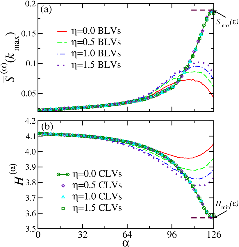
Figure 1: (Color online) Above the SST: (a) Normalized $\bar{S}^{(\alpha)}(k_{\mathrm{max}})$ and (b) spectral entropy $H^{(\alpha)}$ vs. Lyapunov index $\alpha$ corresponding to the BLVs (lines) and CLVs (symbols) for different values of the perturbation parameter $\eta$ of the scalar product (see text). Both plots correspond to the FPU model with $N=128$ and $\varepsilon=10$.

Results.- Our first result concerns the dependence of the significance measure of HLMs on the metric used when constructing the set of backward LVs. Since some scalar product always needs to be defined (for Gram-Schmidt orthonormalization) –and this is to a great extent an arbitrary choice– meaningful conclusions can only be obtained if the significance measures are independent of the chosen scalar product. In order to emphasize the impact of the scalar product when searching for HLMs, we use the scalar product, $\left[\delta\mathbf{q}^{\left(\alpha\right)}\left(t\right);\delta\mathbf{p}^{\left(\alpha\right)}\left(t\right)\right]\mathbb{M}_{2N\times 2N}\left[\delta\mathbf{q}^{\left(\alpha\right)}\left(t\right);\delta\mathbf{p}^{\left(\alpha\right)}\left(t\right)\right]^{T}$, with the matrix $(\mathbb{M})_{i,j}=\delta_{i,j}+\eta\;\delta_{i\leq N,j\leq N}$, $\eta$ being an arbitrary constant. This corresponds to the perturbed Euclidean norm $\sqrt{(\delta\mathbf{q})^{2}(1+\eta)+(\delta\mathbf{p})^{2}}$. We computed the BLVs and CLVs for different choices of $\eta$ and the results for the measures $\bar{S}^{\alpha}(k_{\mathrm{max}})$ and $H^{(\alpha)}$ for the FPU model in the strongly chaotic regime for a high energy density $\varepsilon=10$ are presented in Fig. 1. For both sets of vectors it is clear that $\bar{S}^{\alpha}(k_{\mathrm{max}})$ presents a maximum and $H^{(\alpha)}$ a minimum for some index $\alpha_{\mathrm{max}}$. The curve in Fig. 1(a) for the BLV with $\eta=0$ corresponds to the mode reported in Ref. FPUHLM as a truly HLM for the FPU system. However, note that $\alpha_{\mathrm{max}}\approx 102$ is still far from $126$ by $20\%$, which is the Lyapunov index value corresponding to the smallest positive LE. This deviation was attributed in Ref. FPUHLM to fluctuations of finite-time LEs. We claim that this mode is not a good HLM. As clearly seen in Fig. 1(a), BLV curves exhibit an $\alpha_{\mathrm{max}}$ that progressively shifts as $\eta$ increases, demonstrating that the mode is not intrinsic and its position strongly depends on the employed scalar product. In contrast, if CLVs are used instead, the positions of the extrema, as well as the significance measures $\bar{S}^{(\alpha)}(k_{\mathrm{max}})$ and $H^{(\alpha)}$, are independent of the $\eta$ value used, as confirmed by Fig. 1. Also, the positions of both extrema are located at LE index $\alpha_{\mathrm{max}}\approx 126$, exactly where the smallest positive LE is located. These results indicate that only CLVs can generically detect the existence of intrinsic (scalar-product independent) HLMs. This becomes even clearer if we compute the significance measures $\bar{S}^{(\alpha)}(k_{\mathrm{max}})$ and $H^{(\alpha)}$ for energy densities well below the SST, which is around $\varepsilon_{c}\approx 0.20$ for the FPU FPUHLM (note also an earlier estimate of $\varepsilon_{c}\approx 0.12$ casetti93 ). In this weakly chaotic regime it has been reported that HLMs fail to exist FPUHLM ; XYHLM . In Fig. 2 we plot $\bar{S}^{(\alpha)}(k_{\mathrm{max}})$ and $H^{(\alpha)}$ for an extremely low energy density $\varepsilon=0.01$, where the system behaves almost as a harmonic oscillator chain. As can be readily seen, if CLVs are used, the maximum of $\bar{S}^{(\alpha)}(k_{\mathrm{max}})$ corresponds to the minimum of $H^{(\alpha)}$ at the Lyapunov index $\alpha_{\mathrm{max}}\approx 120$. Thus covariant HLMs exist even well below the SST. In contrast, BLVs fail to detect any significant HLMs for $\varepsilon=0.01$ (actually, for any energy density below $\varepsilon_{c}$), which again indicates that BLVs are unreliable objects whereby to detect HLMs.

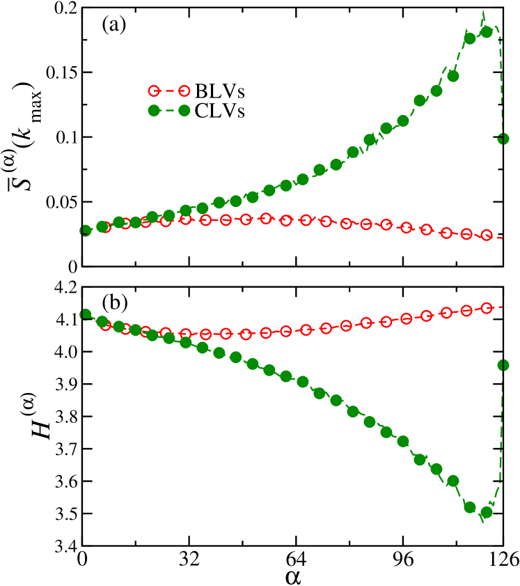
Figure 2: (Color online) Below the SST: (a) $\bar{S}^{(\alpha)}(k_{\mathrm{max}})$ and (b) spectral entropy $H^{(\alpha)}$ vs. the LV index $\alpha$ for the BLVs (open circles) and CLVs (filled circles). Both plots correspond to the FPU model with $N=128$, energy density $\varepsilon=0.01$, and $\eta=0$.

We can now quantify the significance of the HLMs as a function of the energy density by plotting in Fig. 3 the extreme values $S_{\mathrm{max}}$ and $H_{\mathrm{min}}$ indicated in Fig. 1. The energy dependence of these extreme values also shows striking differences when BLVs or CLVs are used. Again, different scalar products lead to different curves if BLVs are used. GS HLMs seem to appear only above some energy density. Indeed, a crossover toward an increasing significance of HLMs is observed as the energy density increases. However, as shown in Fig. 3, the curves for BLVs display a crossover that shifts toward lower $\varepsilon$ values as $\eta$ increases. Thus, the relation of this crossover point with the SST $\varepsilon_{c}$, first conjectured in Ref. FPUHLM , turns out to be an artifact that arises from the use of BLVs, since its position explicitly depends on the employed scalar product. In contrast, the maximum power $S_{\mathrm{max}}(\varepsilon)$ and minimum spectral entropy $H_{\mathrm{min}}(\varepsilon)$ remain constant for the full range of energy densities if CLVs are used to identify HLMs. Figure 3 summarizes our main result: covariant HLMs do exist and their significance, in qualitative and quantitative terms, is the same for the whole range of energy densities studied, irrespective of whether we are above or below the SST.

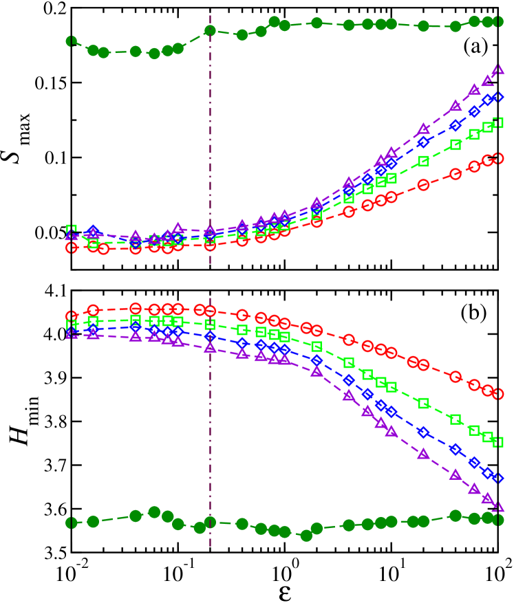
Figure 3: (Color online) (a) $S_{\mathrm{max}}$ and (b) $H_{\mathrm{min}}$ vs. energy density $\varepsilon$ for the BLVs using different scalar products (see text): $\eta=0$ (open circles), $\eta=0.5$ (squares), $\eta=1$, (diamonds) and $\eta=1.5$ (triangles). Data points computed by means of the CLVs are shown with filled circles, and vertical dot-dashed lines indicate the position of the SST according to Ref. FPUHLM .

Next we briefly discuss our results for the $XY$ model consisting of a one-dimensional lattice of interacting rotors. For large enough energy densities, individual particles become nearly independent and the system is close to a collection of free rotors, whereas for small energy densities the system is in a near-harmonic regime, analogous to the corresponding one in the FPU model. We have studied the existence of HLMs in the $XY$ model and obtained results that are qualitatively similar to those in the FPU case. In the high energy density regime the interaction potential is not strong enough to maintain the needed coupling between neighboring rotors; thus spatially extended perturbations cannot be supported by the system dynamics and no HLMs were observed in this regime. In the opposite limit of extremely low energy densities we found no HLMs if BLVs are used, in agreement with an earlier study XYHLM ; however, covariant HLMs do exist even for a low energy density of $\varepsilon=0.1$, as can be appreciated in Fig. 4. The numerical values of the significance measures depend again on the scalar product if BLVs are used, while no effect is seen for CLVs, as expected from our discussion of the FPU case. This confirms our finding that strong chaos is not essential for the appearance of genuine covariant HLMs.

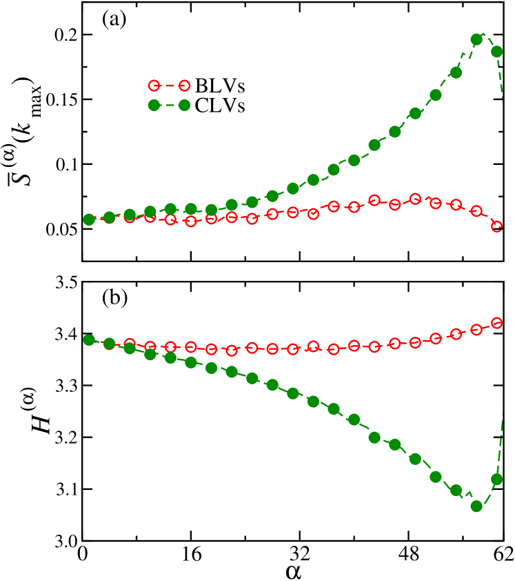
Figure 4: (Color online) (a) Maximum power spectrum $\bar{S}^{(\alpha)}(k_{\mathrm{max}})$ and (b) spectral entropy $H^{(\alpha)}$ for the $XY$ model with $N=64$, $\varepsilon=0.1$, and $\eta=0$, well below the SST.

Conclusions.- We have studied HLMs in Hamiltonian lattices and compared covariant with backward LVs. There are strong theoretical arguments which suggest that HLMs are associated with the existence of conservation laws and translational invariance mcnamara01 ; wijn04 ; CMLHLM2 of the equations of motion. These exact symmetries are thus expected to be satisfied irrespective of the energy density. We have shown that covariant HLMs indeed exist for any energy density so that strong chaos is not an essential requirement for the appearance of genuine HLMs. Actually, the significance of covariant HLMs remains constant both above and below the SST, which seems to indicate that the mechanisms held responsible of the existence of both phenomena should be entirely different. We have also demonstrated that BLVs lead to misleading results concerning the existence of good HLMs and to significance measures that display an undesired dependence on the scalar product.

The spatial structure of the covariant HLMs herein studied indicates that these extended modes have a scale-invariant structure, which contrasts with the truly wavelike spatially periodic form characteristic of hard-core systems posch00 ; eckmann00 ; mcnamara01b ; mcnamara04 ; wijn04 ; forster05 ; tanigu05 ; morriss09 ; chung11 . It remains to be understood whether the extended modes in these two types of systems actually belong to the same kind of phenomenon, and whether these modes can be related to hydrodynamic properties for arbitrary systems with extended chaos.

- (1) H. A. Posch and R. Hirschl, in Hard Ball Systems and the Lorentz Gas, edited by D. Szász (Springer, Berlin, 2000).
- (2) J.-P. Eckmann and O. Gat, J. Stat. Phys. 99, 775 (2000).
- (3) S. McNamara and M. Mareschal, Phys. Rev. E 64, 051103 (2001).
- (4) M. Mareschal and S. McNamara, Physica D 187, 311 (2004).
- (5) A. S. Wijn and H. van Beijeren, Phys. Rev. E 70, 016207 (2004).
- (6) C. Forster and H. A. Posch, New J. Phys. 7, 32 (2005).
- (7) T. Taniguchi and G. P. Morriss, Phys. Rev. Lett. 94, 154101 (2005).
- (8) G. P. Morriss and D. Truant, J. Stat. Mech. P02029 (2009).
- (9) T. Chung, D. Truant, and G. P. Morriss, Phys. Rev. E 83, 046216 (2011).
- (10) H.-L. Yang and G. Radons, Phys. Rev. Lett. 96, 074101 (2006).
- (11) H.-L. Yang and G. Radons, Phys. Rev. E 73, 016202 (2006).
- (12) H.-L. Yang and G. Radons, Phys. Rev. Lett. 100, 024101 (2008).
- (13) S. McNamara and M. Mareschal, Phys. Rev. E 63, 061306 (2001).
- (14) H.-L. Yang and G. Radons, Phys. Rev. E 73, 066201 (2006).
- (15) H.-L. Yang and G. Radons, Phys. Rev. E 77, 016203 (2008).
- (16) H. Kantz, Physica D 39, 322 (1989).
- (17) M. Pettini and M. Cerruti-Sola, Phys. Rev. A 44, 975 (1991).
- (18) M. Pettini and M. Landolfi, Phys. Rev. A 41, 768 (1990).
- (19) E. Fermi, J. Pasta, and S. Ulam (with M. Tsingou), Collected Papers of Enrico Fermi (University of Chicago Press, Chicago, 1965), p. 978.
- (20) M. Pettini et al., Chaos 15, 015106 (2005).
- (21) S. V. Ershov and A. B. Potapov, Physica D 118, 167 (1998).
- (22) G. Benettin, L. Galgani, A. Giorgilli, and J.-M. Strelcyn, Meccanica 15, 9 (1980).
- (23) I. G. Szendro, D. Pazó, M. A. Rodríguez, and J. M. López, Phys. Rev. E 76, 025202(R) (2007).
- (24) D. Pazó, I. G. Szendro, J. M. López, and M. A. Rodríguez, Phys. Rev. E 78, 016209 (2008).
- (25) B. Legras and R. Vautard, in Proceedings of the Seminar on Predictability, Vol. I, ECWF Seminar 1995, edited by T. Palmer (ECMWF, Reading, UK, 1996), pp. 135–146.
- (26) J.-P. Eckmann and D. Ruelle, Rev. Mod. Phys. 57, 617 (1985).
- (27) C. L. Wolfe and R. M. Samelson, Tellus Ser. A 59, 355 (2007).
- (28) H.-L. Yang and G. Radons, Phys. Rev. E 82, 046204 (2010).
- (29) M. Romero-Bastida, D. Pazó, M. A. Rodríguez, and J. M. López, Phys. Rev. E 82, 036205 (2010).
- (30) M. Romero-Bastida and E. Braun, J. Phys. A: Math. Theor. 41, 375101 (2008).
- (31) L. Casetti and M. Pettini, Phys. Rev. E 48, 4320 (1993).