Gaps in Protoplanetary Disks as Signatures of Planets: I. Methodology and Validation

Abstract

We examine the observational consequences of partial gaps being opened by planets in protoplanetary disks. We model the disk using a static $\alpha$-disk model with detailed radiative transfer, parametrizing the shape and size of the partially cleared gaps based on the results of hydrodynamic simulations. Shadowing and illumination by stellar irradiation at the surface of the gap leads to increased contrast as the gap trough is deepened by shadowing and cooling and the far gap wall is puffed up by illumination and heating. In calculating observables, we find that multiple scattering is important and derive an approximation to include these effects. A gap produced by a 200 $M_{\earth}$ (70 $M_{\earth}$) planet at 10 AU can lower/raise the midplane temperature of the disk by up to $\sim-25/+29\%$ ($\sim-11/+19$) by shadowing in the gap trough and illumination on the far shoulder of the gap. At the distance of Taurus, this gap would be resolvable with $\sim 0.01\arcsec$ angular resolution. The gap contrast is most significant in scattered light and at thermal continuum wavelengths characteristic of the surface temperature, reducing or raising the surface brightness by up to order of magnitude. Since gaps sizes are correlated to planet mass, this is a promising way of finding and determining the masses of planets embedded in protoplanetary disks.

1. Introduction

With the advent of adaptive optics systems on large ground-based optical and near-IR telescopes, we are beginning to be able to image protoplanetary disks around young stars (e.g.  Thalmann et al., 2010, LkCa 15). These gas-rich disks are where we expect giant planets to form, since gas giants need that large reservoir of gas from which to accrete their massive envelopes. However, the interpretation of structure in these imaged disks can be problematic, because scattered light traces only the optically thin and diffuse surface layers of the disks rather than the overall structure of the disk (Jang-Condell & Boss, 2007). On the other hand, if growing planets do indeed significantly perturb the disks in which they are born, observation of these signatures can mean the detection of nascent planets in protoplanetary disks.

Jang-Condell (2008, henceforth JC08) calculated the shape of a dimple created by the gravitational potential of a planet embedded in a disk and the accompanying thermal perturbations in shadowed and illuminated regions of the dimple. Jang-Condell (2009, henceforth JC09) predicted the observability of these dimples. Neither of the papers considered the clearing of an annular gap in the disk by tidal forces. Planets above about 30 M_⊕ are able to open partial gaps in disks, as demonstrated in numerical hydrodynamic simulations (e.g. Bate et al., 2003). These gaps are much larger in scale than the local dimples modeled in JC08 and JC09 and are therefore a promising way of detecting and characterizing planets in protoplanetary disks. If the gap is well resolved enough to determine its depth and width, then we can determine the mass of the planet to within a factors of a few.

JC09 considered only single scattering and direct thermal emission to calculate observable signatures of disk perturbations. However, multiple scattering, particularly at high albedos, can significantly increase disk brightnesses. While Monte Carlo methods directly calculate multiple scattering, they are computationally intensive so that iteratively calculating the disk structure is prohibitively time consuming (e.g.  Walker et al., 2004; Dullemond & Dominik, 2004; Tannirkulam et al., 2008; Pinte et al., 2008; Mulders et al., 2010). The approach here is to exploit a few analytic approximations to the solutions of the radiative transfer equations to efficiently calculate the disk structure.

Numerous people have carried out hydrodynamic simulations of gap opening in disks by planets (e.g. Paardekooper & Papaloizou, 2008; Ayliffe & Bate, 2009; de Val-Borro et al., 2006; Bate et al., 2003; Edgar & Quillen, 2008) However, the effects of illumination of these gaps by the central star has not been well-studied. Wolf et al. (2002) examine this problem in a flat disk with constant $H/r=0.05$ and find that the far edge of the gap is not illuminated. On the other hand, Varnière et al. (2006) find that the far edge in a flared disk, which is more typical of T Tauri disks, is heated and puffed up, creating a positive feedback loop that enhances the appearance of the gap. In both these cases, the gap was created by a Jupiter-mass planet, which clears nearly all the material from its orbital, creating a deep and wide gap. In this work, we focus on partially cleared gaps created by sub-Jupiter mass planets.

A full three-dimensional hydrodynamic simulation including radiative transfer is very computationally intensive, so we simplify the problem by assuming a fixed disk structure in terms of its radial surface density profile, $\Sigma(r)$. To further simplify the computation, we assume an axisymmetric disk structure. This means that we do not include the behavior of spiral density waves, but only the large scale gap opened by the planet.

2. The JC Model

The methods used for calculating radiative transfer in protoplanetary disks for both radiative heating and observable quantities are those used in JC08 and JC09. In this work, we now apply these methods to an axisymmetric disk structure rather than an azimuthally limited local perturbation, and we account for multiple scattering in the observables. We will refer to these methods as the JC model, to constrast to Monte Carlo methods.

The disk model incorporates radiative transfer based on the methods of Jang-Condell & Sasselov (2003) and Jang-Condell & Sasselov (2004) and adopted to self-consistently determine the disks thermal and pressure structure as described in JC08. Stellar irradiation is an important heating source in protoplanetary disks, and the amount of heating is sensitive to the angle of incidence at the disk surface. If the shape of the surface of the disk changes on scales smaller than the disk thickness, the plane-parallel approximation fails. To account for this kind of disk structure, radiative heating is integrated piecewise over the surface of the disk rather than assuming a thin plane-parallel disk model. This method of calculating radiative transfer is fully-three dimensional and not directionally dependent on a fixed coordinate system. More detailed explanation of the method can be found in JC08 and references therein. Calculation of the observables is done as detailed in JC09, with modifications to approximate the effects of multiple scattering, as discussed below. In this section, we summarize the essential features of the model.

2.1. Initial Conditions

We follow the same method as used in JC08 and JC09 to calculate the initial disk structure. The stellar parameters are mass $M_{*}=1\,M_{\odot}$, radius $R_{*}=2.6\,R_{\odot}$, and effective temperature $T_{\mbox{\scriptsize eff}}=4280$ K, consistent with a protostar with an age of 1 Myr (Siess et al., 2000). We assume a constant-$\alpha$ disk model where the viscosity is parameterized as $\nu=\alpha_{\mbox{\scriptsize ss}}c_{s}H$ (Shakura & Sunyaev, 1973). The disk parameters are accretion rate $\dot{M}=10^{-8}\,M_{\sun}\,\mbox{yr}^{-1}$ and viscosity parameter $\alpha_{\mbox{\scriptsize ss}}=0.01$, parameters typical for T Tauri stars.

The initial conditions are calculated in a two-step process. In both steps, we iteratively calculate the density and temperature structure of the disk, including radiative transfer of the stellar irradiation at the disk surface. Viscous heating is included, but is only important inwards of a few AU. Beyond this distance, the primary heating source is stellar irradiation, which depends sensitively on the angle of incidence at the surface of the disk. The surface is defined to be where the Planck-averaged optical depth to stellar irradiation is 2/3.

In step 1, we generate a locally plane-parallel model for the entire disk. For this initial locally plane-parallel model, we calculate the disk at logarithmically spaced intervals of $\sqrt{2}$ from 0.25 AU to 256 AU.

In step 2, we select a radially and azimuthally limited wedge of this disk to calculate in more detail, including the three dimensional curvature of the wedge, but assuming axisymmetry. The model presented here is a slice with radial range ($r$) from 3 to 20.8 AU and vertical distance from the midplane ($z$) from 0 to 5.5 AU in order to model the gap created by at planet at 10 AU. We sample the initial density and temperature at 100 grid points in both $r$ and $z$ directions, using cylindrical coordinates. In order to ensure that that this initial disk is in thermal and hydrostatic equilibrium, we recalculate the heating from stellar irradiation, now removing the assumption that the disk is locally plane parallel and including the full three-dimensional curvature of the disk. The resulting density profile is $\Sigma_{0}(r)$. The total disk mass within the simulation boundaries is 0.0025 $M_{\sun}$.

2.2. Gap Modeling

The depth of a gap that can be opened by a planet depends not only on the mass ratio between planet and star, but also on the disk properties. In a low viscosity disk, the critical threshold for gap-opening is generally considered to be the mass at which the planet’s Hill radius equals the thermal scale height of the disk. The Hill radius is $r_{\mbox{\scriptsize Hill}}=(q/3)^{1/3}a$ where $q\equiv M_{p}/M_{*}$ is the mass ratio of the planet to the star. The thermal scale height is $H=c_{s}/\Omega_{K}$ where $c_{s}\equiv\sqrt{kT/\mu}$ is the thermal sound speed and $\Omega_{K}\equiv\sqrt{GM_{*}/a^{3}}$ is the Keplerian orbital angular speed. Here, $k$ is Boltzmann’s constant; $T$ is the disk’s midplane temperature; $\mu$ is the mean molecular weight of of the gas, assumed to be primarily molecular hydrogen; and $G$ is Newton’s gravitational constant.

The gap opening criterion for a viscous disk has been found empirically to be

$$\frac{3}{4}\frac{H}{r_{\mbox{\scriptsize Hill}}}+\frac{50}{q{\cal R}}\lesssim 1$$ (1)

where Reynolds number is defined as ${\cal R}\equiv r^{2}\Omega_{P}/\nu$ (Crida et al., 2006). Their results are also consistent with those of Varnière et al. (2004).

For the purposes of this paper, we adopt gap profiles similar to those calculated by Bate et al. (2003), who model gap opening by planets of varying masses in a disk using three-dimensional hydrodynamic simulations, focusing specifically on planets that only partially open gaps in disks. A gap is modeled as an ad hoc perturbation imposed on the initial conditions. The surface density of a disk modified by a gap of width $w$, depth $d$, and position $a$ is

$$\Sigma(r)=\Sigma_{0}(r)\left\{1-d\exp[-(r-a)^{2}/(2w^{2})]\right\}.$$ (2)

This is consistent with the results of (Crida & Morbidelli, 2007), who find that planets whose masses are less than that of the disk open local gaps in disks rather than clearing inner cavities. Since the study presented here addresses planets under a Jupiter mass ($M_{J}$), they are well under the disk mass.

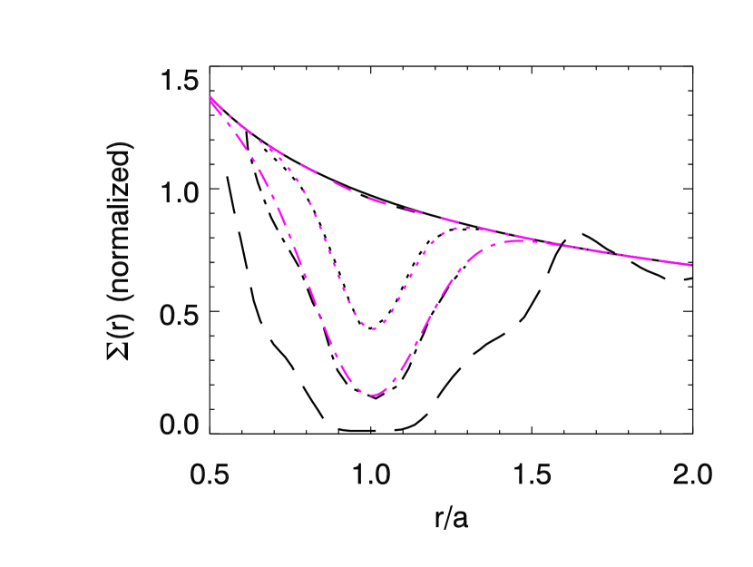
Figure 1.— Profiles of gaps carved by planets in disks and the Gaussian fits to them. The unperturbed disk profile is plotted as a solid line, while the dashed, dotted, dot-dashed, and long-dashed lines are gaps opened by planets of $q=3\times 10^{-5},1\times 10^{-4},3\times 10^{-4},$ and $1\times 10^{-3}$, respectively. The black lines are from Bate et al. (2003), and magenta lines are Gaussian fits, following Eq. (2). The gap opened by the $q=1\times 10^{-3}$ planet is not well fit by a a Gaussian.

The depth and width of the gap compared to planet mass are determined from the results of Bate et al. (2003). In Figure 1, we reproduce the surface density profiles of gap opening by planets from Figure 2 of Bate et al. (2003), having used DataThief to acquire the values. The unperturbed density profile is plotted as a solid line, and goes as $\Sigma_{0}(r)\propto r^{-1/2}$. The planet is located at $r/a=1$. The gaps opened by planets of 0.03, 0.1, 0.3 and 1 $M_{J}$ are plotted as dashed, dotted, dot-dashed, and long-dashed black lines, respectively. We fit all but the 1 $M_{J}$ planet to Equation (2), and plot these fits as magenta lines in Figure 1. The best fit parameters are tabulated in Table 1. The maximum deviation between the empirical gap profile and the fit, expressed as a precentage of the unperturbed disk density, is 0.04% for the 0.03 $M_{J}$ planet, 3% for the 0.1 $M_{J}$ planet, and 9% for the 0.3 $M_{J}$ planet. The deviation for the 0.3 $M_{J}$ planet is greatest at $r/a<1$, indicating asymmetry of the gap that is not accounted for in the model presented here. Nevertheless, fitting the gap to a Gaussian is a useful model for parametrizing the disk response to a planet without the need for running a full hydrodynamic simulation.

Table 1Best-fit parameters for gaps opened by planets.

$q$	$d$	$w/a$	max. error	$G$	derived $q$	derived planet mass
$3\times 10^{-5}$	0.014	0.078	0.04%	18	$6.7\times 10^{-5}$	22 $M_{\earth}$
$1\times 10^{-4}$	0.56	0.11	3%	6.2	$2.2\times 10^{-4}$	72 $M_{\earth}$
$3\times 10^{-4}$	0.84	0.17	9%	2.5	$6.2\times 10^{-4}$	210 $M_{\earth}$
$1\times 10^{-3}$	—	—	—	1.0	$1.9\times 10^{-3}$	620 $M_{\earth}$

In (Bate et al., 2003), ${\cal R}=10^{5}$ and $H/a=0.05$. Using Eq. (1) as the gap opening criterion, this gives a gap-opening threshold of $q_{\mbox{\scriptsize crit}}=1.06\times 10^{-3}$, or slightly more than 1 $M_{J}$. For comparison, $r_{\mbox{\scriptsize Hill}}=H$ when $q=3.75\times 10^{-4}$, so the viscous gap opening criterion gives a mass more than twice as large as for an inviscid disk. In the disk model adopted in this paper, at 10 AU the midplane temperature is 50K, $H/r=0.048$, and $\alpha_{\mbox{\scriptsize ss}}=0.01$, so ${\cal R}=4.4\times 10^{4}$ and the gap-opening threshold is $q_{\mbox{\scriptsize crit}}=1.97\times 10^{-3}$, or almost 2 $M_{J}$.

Given the difference in disk properties, we cannot assume that the same mass planets open the same size gaps in each disk. We estimate the masses of planet according to the following procedure. Defining

$$G\equiv\frac{3}{4}\frac{H}{r_{\mbox{\scriptsize Hill}}}+\frac{50}{q{\cal R}},$$ (3)

we assume that $G$ is the relevant scale for determining the depth of the gap opened by a planet, so that planets with the same value of $G$ open similarly sized gaps. Then, the 0.03, 0.1, and 0.3 $M_{J}$ planets in the disk modeled by Bate et al. (2003) have mass ratios of $q=3\times 10^{-5},1\times 10^{-4}$ and $3\times 10^{-4}$, respectively, and have $G$ values as tabulated in Table 1. For the disk parameters adopted in this paper, the equivalent planet masses are then approximately 20, 70 and 200 $M_{\oplus}$, assuming that $M_{\earth}/M_{\sun}=3\times 10^{-6}$.

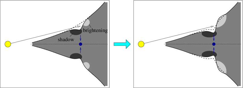
Figure 2.— Cartoon diagram of radiative feedback on disk structure. The star is represented as a yellow disk, and the planet by a blue dot. The disk surface represents a contour of constant density. The left image shows the initial gap opened in the disk, with the dotted line showing the original, unperturbed disk surface. Stellar illumination on the surface of the gap creates shadowed and brightened regions. Shadowing and cooling occurs in the disk trough, and the far side of the gap is illuminated and heated. The right image shows the response of the gaseous disk material to the cooling and heating: the shadowed region contracts and deepens the gap, while the illuminated far side expands and is elevated.

Holding $\Sigma(r)$ constant and assuming axisymmetry, we recalculate the temperature structure of the disk, using the same iterative radiative transfer method as described in §2.1. The effect of the gap is to create a shadow within the trough in density created by the gap. The far side of the gap, which is now exposed to more direct stellar illumination, is brightened. A schematic of this is shown in Figure 2. This results in cooling within the trough and heating on the far wall. The gas that composes the bulk of the disk material responds to this cooling and heating by contracting and expanding. This changes the vertical density profile of the gap region, and the illuminated surface now must be recalculated. For this reason, the heating and cooling of the disk must be calculated self-consistently with the density structure of the disk.

2.3. Observables

Calculation of synthetic images of disks with gaps is done as in JC09, with the addition of including multiple scattering. In our comparisons to Monte Carlo radiative transfer codes, we find that multiple scattering turns out to be an important component of disk emission. Multiple scattering generally has the property of increasing the brightness of a diffuse disk. In the case of high albedos, the additional brightening can be significant. Here, we present an estimate for the brightness due to secondary scattering of both scattered stellar irradiation and thermal emission from the disk. We assume isotropic scattering in these derivations.

2.3.1 Multiple Scattering of Stellar Irradiation

Here we consider pure scattering of stellar photons. From JC09, the intensity of singly scattered light of frequency $\nu$ from the disk surface is

$$I_{1}^{s}(\nu)=\frac{\omega_{\nu}\mu\/R_{*}^{2}\/B_{\nu}(T_{*})}{4r^{2}(\mu+\cos\eta)},$$ (4)

where $\omega_{\nu}$ is the albedo, $B_{\nu}(T_{*})$ is the intensity emitted at the stellar surface (here assumed to be a blackbody), $r$ is the distance from the star, $\mu$ is the cosine of the angle of incidence of stellar light, and $\eta$ is the angle between the line of sight to the observer and normal to the surface. The angle $\eta$ is distinct from the inclination angle of the overall disk, which we represent as $i$. The angles are illustrated in Figure 3.

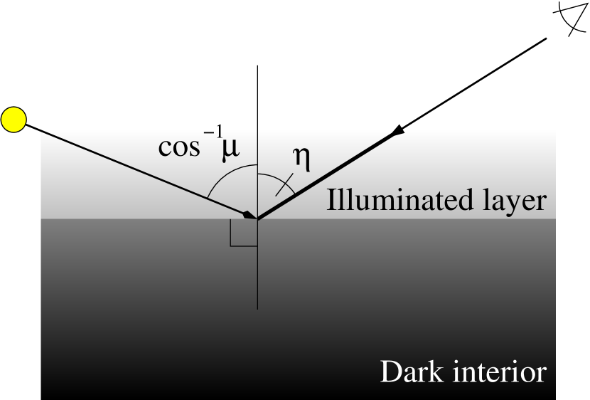
Figure 3.— Illustration of how inclination affects brightness of scattered light. The path length through the illuminated layer represents the relative brightness seen by each observer. The cosine of the angle of incidence of stellar light at the surface is $\mu$. The angle between the surface normal and the observer is $\eta$.

For multiply scattered photons, we first need to determine the diffuse scattered radiation field within the disk, $J_{s}$. This was solved for in Jang-Condell & Sasselov (2003, 2004) using plane-parallel equations for radiative transfer as

$$J_{s} = \frac{B_{\nu}(T_{*})R_{*}^{2}}{4l^{2}}\frac{\mu\omega_{\nu}}{1-3g^{2}\mu^{2}}$$ (5)

$$\quad\times\left[\frac{2+3\mu}{1+2g/3}\exp(-g\tau_{\perp})-3\mu\exp(-\tau_{\perp}/\mu)\right]$$

where $g=\sqrt{3(1-\omega_{\nu})}$ (see also D’Alessio et al. (1998)).

Given $J_{s}$, then the brightness of photons scattered to the observer after two or more scatterings is

$$I_{2}^{s}(\nu)=\int_{0}^{\infty}\omega_{\nu}\exp(-\tau_{\mbox{\scriptsize obs}})J_{s}\,d\tau_{\mbox{\scriptsize obs}}$$ (6)

where $\tau_{\mbox{\scriptsize obs}}$ is the line-of-sight optical depth. If $\tau_{\perp}$ is the optical depth perpendicularly below the surface of the disk, and $\eta$ is the angle of the observer with respect to the disk normal, then $\tau_{\mbox{\scriptsize obs}}=\tau_{\perp}/\cos\eta$. Then,

$$I_{2}^{s} = \frac{B_{\nu}(T_{*})R_{*}^{2}}{4l^{2}}\frac{\mu\omega^{2}}{1-g^{2}\mu^{2}}\times$$ (7)

$$\quad\left[\frac{2+3\mu}{(1+2g/3)}\frac{1}{(1+g\cos\eta)}-\frac{3\mu}{(1+\cos\eta/\mu)}\right]$$

and

$$I_{\nu}^{s} = I_{1}^{s}+I_{2}^{s}=\frac{\omega_{\nu}\mu\/R_{*}^{2}\/B_{\nu}(T_{*})}{4r^{2}(\mu+\cos\eta)}\times$$ (8)

$$\quad\left\{1+\frac{\omega}{1-g^{2}\mu^{2}}\left[\frac{(2+3\mu)(\mu+\cos\eta)}{(1+2g/3)(1+g\cos\eta)}-3\mu^{2}\right]\right\}.$$

2.3.2 Scattered Thermal Emission

Assuming a plane-parallel disk atmosphere, the radiative transfer equation is

$$\cos\eta\frac{\partial I_{\nu}}{\partial\tau_{\nu}}=I_{\nu}-S_{\nu}$$ (9)

where $\eta$ is the viewing angle with respect to the line perpendicular to the disk, and $\tau_{\nu}$ is the total extinction perpendicular to the surface, including both absorption and scattering. For scattering and absorption, the source function is

$$S_{\nu}=\omega_{\nu}J_{\nu}+(1-\omega_{\nu})B_{\nu}$$ (10)

where $\omega_{\nu}$ is the wavelength-dependent albedo and $B_{\nu}=B_{\nu}(T)$ is the local thermal emission. Adopting the Eddington approximation,

$$\frac{1}{3}\frac{\partial^{2}J_{\nu}}{\partial\tau_{\nu}^{2}}=(1-\omega_{\nu})(J_{\nu}-B_{\nu}).$$ (11)

We have $B_{\nu}$ from the temperature structure of the disk, and we can integrate Eq. 11 to get $J_{\nu}$. Finally, we integrate Eq. 9 to get the emitted intensity at the surface of the disk.

In the case of an isothermal slab of finite optical thickness ($\tau_{\mbox{\scriptsize max}}$), we can set the boundary conditions at $\tau=0$ and $\tau=\tau_{\mbox{\scriptsize max}}$

$$J_{\nu}(\tau=0) = \frac{1}{\sqrt{3}}\frac{\partial J}{\partial\tau}(\tau=0)$$ (12)

$$J_{\nu}(\tau=\tau_{\mbox{\scriptsize max}}) = -\frac{1}{\sqrt{3}}\frac{\partial J}{\partial\tau}(\tau=\tau_{\mbox{\scriptsize max}})$$ (13)

(Rybicki & Lightman, 1979). Solving,

$$J_{\nu} = B_{\nu}(T)\left\{1\right.$$

$$\left.-\frac{\exp\left[(\tau-\tau_{\mbox{\scriptsize max}})\sqrt{3(1-\omega_{\nu})}\right]+\exp\left[-\tau\sqrt{3(1-\omega_{\nu})}\right]}{\left(1-\sqrt{1-\omega_{\nu}}\right)\exp\left[-\tau_{\mbox{\scriptsize max}}\sqrt{3(1-\omega_{\nu})}\right]+1+\sqrt{(1-\omega_{\nu})}}\right\}.$$

If we assume that $T$ varies slowly with $\tau$, then we can approximate $J_{\nu}$ by Eq. (2.3.2) locally, as done in D’Alessio et al. (2001) Then the emergent intensity can be found by integrating Eq. (9), assuming that the background intensity is $0$. To simplify the calculation, we assume that the disk is locally plane parallel, so $\eta=i$, the inclination angle. For a face on disk, $\eta=0$.

The total intensity is then $I_{\nu}=I_{\nu}^{s}+I_{\nu}^{t}$, although as a general rule $I_{\nu}^{2}$ dominates in optical to mid-IR, and $I_{\nu}^{t}$ dominates at longer wavelengths.

3. Validation

The JC radiative transfer model for calculating the disk structure for this work is fully three-dimensional, in the sense that radiation impinging on the surface of the disk is allowed to propagate in all directions throughout the disk. However, it relies on a locally one-dimensional analytic solution to the radiative transfer equation and adopts a number of simplifying assumptions such as mean opacities (see also Jang-Condell & Sasselov, 2003, 2004). The novel approach presented in this paper is the iterative calculation of the self-consistent density and temperature structure. As shown by the significant temperature perturbations created by shadowing and illumination on gaps, the self-consistency is an important aspect to consider in the analysis of radiative transfer in disks.

In order to validate the radiative transfer prescription adopted in this paper, we compare our results to a Monte Carlo radiative transfer calculation on the final disk density structure (Turner et al., 2011). The Monte Carlo approach is similar to that of Pinte et al. (2006). We find the radiative equilibrium temperatures by following a large number of photon packets from the star through scattering, absorption and re-emission until escape to infinity. In this way the energy is conserved exactly. We sum the radiation energy absorbed all along the packet paths (Lucy, 1999) and relax to equilibrium by choosing each re-emitted packet’s frequency to adjust the local radiation field for the updated temperature (Bjorkman & Wood, 2001). The scattering is assumed to be isotropic. Each of the calculations shown involves $10^{9}$ photon packets.

In the following section, as we discuss our results for the disk temperature structure and observable quantities, we compare the JC model to the results found by the Monte Carlo (MC) method.

4. Results

4.1. Gap Structure

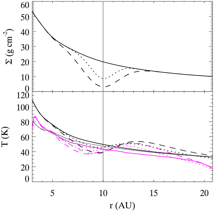
Figure 4.— Surface density (top) and midplane temperature (bottom) profiles for a disk with and without a gap created by a planet at 10 AU. Solid, dotted, and dashed lines indicate planet masses of 0, 70, and 200 $M_{\oplus}$, respectively. The thermal perturbation is caused by shadowing and illumination by stellar irradiation at the disk surface. The black lines indicate the results of the JC models while the gray lines show JC models excluding viscous heating at the midplane. The magenta lines on the temperature plot show the results of a Monte Carlo radiative transfer calculation on the same three-dimensional density structure.

The surface density profiles imposed on the disk for 0, 70, and 200 $M_{\earth}$ planets are shown in the upper plot of Figure 4, as solid, dotted, and dashed lines, respectively. The calculated midplane temperatures for the corresponding disk models are summarized in the lower plot of Figure 4, in black for the JC models, and in magenta for the MC calculations.

The Monte Carlo calculations include only the disk annulus between cylindrical radii 3 and 20.8 AU. For computational speed, the highly optically-thick material within 3 AU is omitted. Without the obscuring material, the wall facing the star at 3 AU would become unexpectedly hot. We mitigate this by immediately discarding any Monte Carlo photon packet absorbed or scattered for the first time in the innermost column of grid cells. Some residual excess heating comes from the fact that omitting the inner disk reduces the column to the star even in the atmosphere, where the innermost cells are optically-thin. This residual excess is significant only inside about 4 AU. On the other hand, truncating the disk model at the outer radius reduces temperatures, since photon packets reaching 20.8 AU can escape to infinity, radiatively cooling the midplane. Considering these approximations together, we believe the Monte Carlo results between 4 and 18 AU accurately represent the solution that would be obtained at greater computational expense in a disk model continuing inward to the sublimation radius and outward to the disk’s far edge.

The JC temperature is consistently higher than the MC temperatures overall. One cause of this discrepancy is that the JC model includes viscous heating at the midplane, so that the final temperature is

$$T=(T_{r}^{4}+T_{v}^{4})^{1/4}$$ (15)

where $T_{r}$ and $T_{v}$ are the temperatures resulting from stellar irradiation and viscous heating, respectively. The viscous temperature is given by

$$T_{v}^{4}=\frac{9}{32\pi}\frac{GM_{\star}\dot{M}}{\sigma_{B}r^{3}}\left[1-\left(\frac{R_{\star}}{r}\right)^{1/2}\right](\tau_{d}+2/3)$$ (16)

where $\sigma_{B}$ is the Stefan-Boltzmann constant and $\tau_{d}$ is the vertically integrated optical depth, $\tau_{d}=-\int_{\infty}^{z}\chi_{R}\rho\,dz$, with respect to $\chi_{R}$, the Rosseland mean opacity.

In Figure 4, we plot $T_{r}$ in grey to show the effect of removing viscous heating. Viscous heating contributes more at smaller $r$, and is neglible beyond $\sim$15 AU. Interior to 5 AU, $T_{r}$ is less than that calculated by the MC model, and outside of 5 AU, the MC temperatures fall more rapidly than the JC temperatures. Thus, viscous heating can explain the discrepant temperatures only at small radii. Another possible explanation is that the difference lies in the treatment of opacities in the two models, as will be described below.

The gap opened by the 20 M_⊕ planet is less than 2% in depth, and produces no more than 2% excursions in temperature from the unperturbed disk, so small as to be negligible. We thus set 20 M_⊕ as the lower bound on a detectable planet in this disk at 10 AU, or more generally, planets with $q\leq 0.036\,q_{\mbox{\scriptsize crit}}$ or $G\geq 18$ are undetectable, whereas planets with $q\geq 0.12\,q_{\mbox{\scriptsize crit}}$ or $G\leq 6$ do significantly perturb the disk.

In contrast to the results of JC08, the midplane temperature is significantly affected by gap opening. JC08 considered planets up to 50 $M_{\oplus}$ in the absence of a gap, but here we find that a 70 $M_{\oplus}$ planet should open a significant gap. In a disk with lower viscosity, a 50 $M_{\oplus}$ might open a similarly sized gap. This shows the importance of including large scale non-linear dynamical interactions in planet-disk models.

Figure 4 illustrates that a gap in a disk creates an S-shaped perturbation to the midplane temperature profile. The temperature at the position of the planet is lowered, although the temperature minimum is inward of the planet position. This is because cooling at the gap minimum is mitigated by heating on the far gap wall. In the JC model, the minimum and maximum temperature deviations at the midplane for the 70 $M_{\oplus}$ planet are $-6$ K ($-11\%$) at 8.9 AU and $+8$ K ($+19\%$) at 13.4 AU, respectively. In the MC model, these values are $-6$ K ($-13\%$) at 8.0 AU and $+9$ K ($+25\%$) at 13.1 AU, respectively. For the 200 $M_{\earth}$ planet, the values are $-13$ K ($-25\%$) at 9.1 AU and $+12$ K ($+29\%$) at 13.9 AU in the JC model, and $-11$ K ($-23\%$) at 7.9 AU and $+14$ K ($+38\%$) at 13.4 AU. In general, the magnitude of heating and cooling in Kelvins is comparable, but the percentages differ because the unperturbed temperature of the MC model is smaller. The positions of the minima and maxima in the JC model are slightly inward of the minima and maxima in the MC model, which might be caused by the same reasons that give rise to the lower midplane temperatures in the MC model.

The full radial and vertical temperature structure of our models are shown in Figure 5. The vertical axis is stretched compared to the horizontal axis in these plots. The top, middle, and bottom plots show gaps created by 0, 70, and 200 $M_{\earth}$ planets, respectively. The JC models are plotted in black, while the MC models are plotted in magenta.

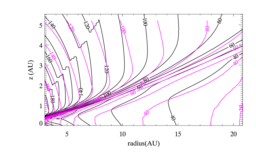
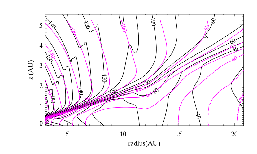
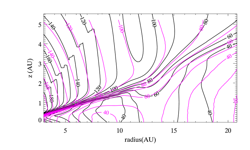
Figure 5.— Temperature cross-sections of disk models with and without gaps. Black and magenta lines show the JC and MC methods, respectively, of calculating radiative heating. Top: A disk without a planet or a gap. Middle: A disk with a gap created by a 70 $M_{\earth}$ planet. Bottom: A disk with a gap created by a 200 $M_{\earth}$ planet.

The abrupt shifts in temperature in the upper left corners of the JC model are purely a numerical artifact. This region is extremely low density, so this region is considered to be outside the bounds of the simulation, and the temperature is assigned based on zero optical depth and a radial dependence. Since these regions are very low density, the temperature differences have no effect on hydrostatic equilibrium nor on the observables, and do not affect the remainder of the analysis presented in this paper, though the topic should be addressed in future studies.

The disk surface is coincident with regions where the temperature changes rapidly in the vertical direction, i.e. where the temperature contours lie close together. Above the surface, the JC model is generally warmer than the MC model. However, at or just below the surface, the MC model is generally warmer. Closer to the midplane, the JC model again becomes warmer, as discussed previously. The warmer temperatures in the MC model below the disk surface indicate that heating by stellar irradiaton penetrates deeper in the MC model than the JC model. The probable cause of this and other differences in temperatures between models, is that the JC model calculates the propagation of stellar photons into the disk using mean opacities, which treats all stellar photons as if they have the same opacity. In the MC models, opacity varies with wavelength, so photons with wavelengths longward of the stellar peak have a lower opacity and can heat the disk to deeper depths. The inclusion of viscous heating in the JC model leads to the increase in temperature at the midplane.

When a gap is imposed on the disk, as in the lower two plots of Figure 5, shadowing and cooling within the gap resulting in the temperature contour lines dipping downward. The depth of these dips are comparable in both the JC and MC models, although the exact shape differs. This difference may again be explained by the the choice of mean opacities versus wavelength-dependent opacities. Allowing longer wavelength photons to penetrate further into the disk would have the effect of smearing out the temperature differences casued by surface effects.

A close look at the surface temperature contours at $r>20AU$ reveals that the surface temperatures are lower for the a gapped disk in both the JC and MC models. This is a result of shadowing of the outermost radii by the puffed up outer edge of the gap. This shadowing and cooling effect is quite real, but since the shadow extends beyond the simulation boundaries, quantifying this effect further is beyond the scope of this paper. A similar shadowing by the illuminated outer edge of a gap created by Jupiter by Turner et al. (2011).

4.2. Simulated Images

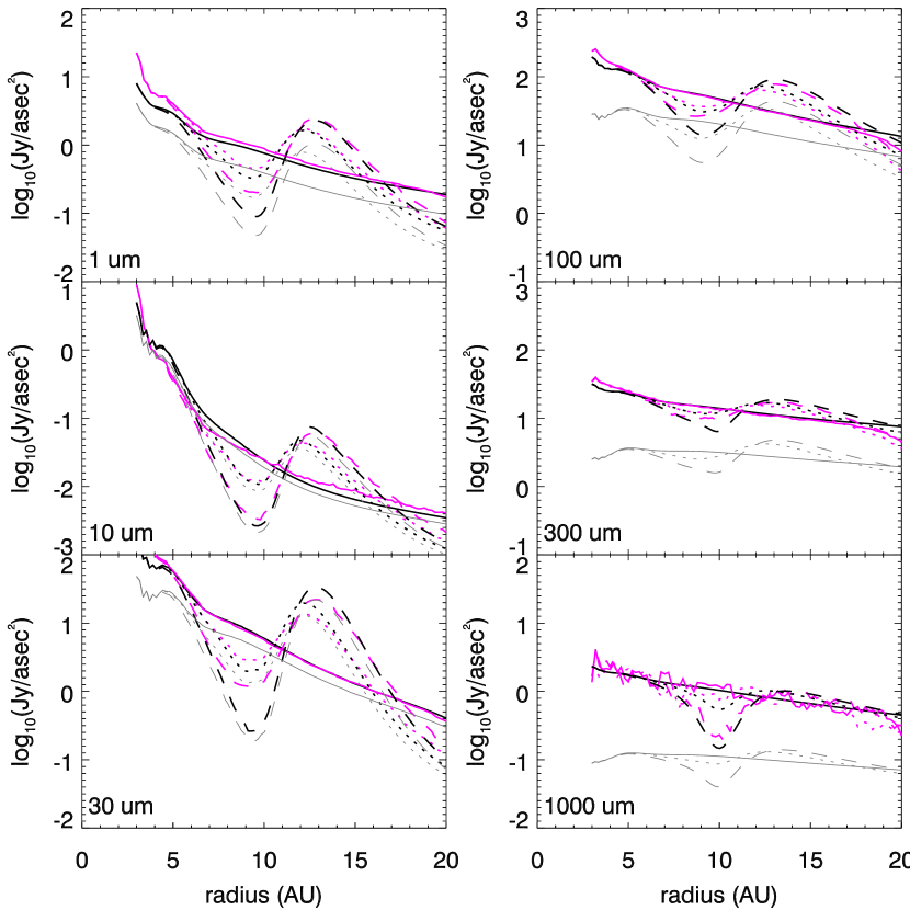
Figure 6.— Radial surface brightness profiles of face-on disks with and without gaps at the wavelengths imaged in Figures 7 & 8, as indicated. The gapless disk surface brightness are plotted with solid lines. Surface brightness profiles of gaps created by 70 and 200 $M_{\oplus}$ planet are plotted as dotted and dashed lines, respectively. Black lines indicate the JC models including multiple scattering, while gray lines show only single scattering or direct emission. For comparison, results from MC calculations on the identical disk density structure are overplotted as magenta lines. The 1 mm brightness profiles is noisy because of low photon statistics. MC calculations give consistently higher brightnesses because of multiple scattering and temperature differences, as discussed in the text,

The radial surface brightness profiles for each of the disks are shown in Figure 6 at wavelengths of $1-1000$ $\mu$m. The JC models are plotted in black, and the Monte Carlo models are plotted in magenta. The brightness profiles of the unperturbed disk are plotted as solid lines, and gaps created by 70 and 200 $M_{\earth}$ planets are plotted as dotted and dashed lines, respectively. We show general good agreement between the models. The noise in the brightness profiles at 1000 microns in the MC models is caused by low photon statistics. This is because the 1000 microns wavelength lies out in the tail of the thermal distribution. Most photon packets have wavelengths near the peak emission of star or disk.

For comparison, we plot as gray lines in Figure 6 the JC brightness profiles for single scattering and direct thermal emission only, as calculated in JC09. Inclusion of multiple scattering of both scattered stellar photons and thermally emitted photons bring the JC brightness profiles in line with the MC ones. At 1 micron, the albedo is $\omega_{\nu}=0.91$ and the disk emission is effectively purely scattered light, so the disk about twice as bright. At 10 microns, $\omega_{\nu}=0.45$, and scattered photons and thermally emitted photons are roughly equal. Because of the relatively low albedo, multiple scattering increases the brightness by about $30\%$ averaged over radius. At 30 microns, $\omega_{\nu}=0.45$ also, but because thermal emission is dominant at the wavelenght, the overall brightness is increased by about $70\%$. Multiple scattering is more effective at increasing thermal emission because it allows photons emitted in optically thick regions to percolate up through the disk. Scattered light, on the other hand, is limited to the photons incident on the surface of the disk. As the albedo increase, the amount of brightening increases: at 100, 300, and 1000 microns, the $\omega_{\nu}=0.57,0.82,$ and $0.95$, and the brightness is increased by factors of $2.6$, $4.9$, and $9.8$, respectively, as averaged over radius.

The perturbation from the gap shadow is evident across all wavelengths, reflecting the cooling and heating that take place in the shadowed trough and brightened rim of the gap. The puffing up of the far rim of the gap is significant enough to shadow and cool the outer disk, as evident in the steeping of the brightness profile toward 20 AU at $1-100$ microns. The brightening of the far rim of the gap in the 1 $\mu$m brightness profile is consistent with the results of Varnière et al. (2006), with feedback from cooling and shadowing resulting in a puffing up of the gap edge.

Despite the offset in the midplane temperature maxima and minima, the appearance of the gap at all wavelengths is consistent. The JC model tends to overpredict the depth of the gap, particularly at 1 micron, and from $30-300$ microns. At 1 micron, this maybe because photons can scatter from the back wall of the gap into the gap, and this is not captured in the JC model. From $30-300$ microns, the difference may arise from the detailed differences in the gap temperature structure between the JC and MC models. At least qualitatively the models agree.

Having validated the JC model by comparison to the MC model, the remainder of our analysis will focus on the JC model.

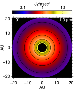
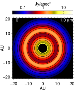
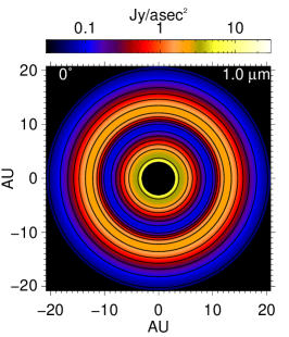
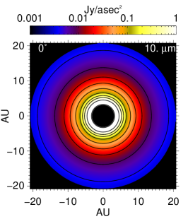
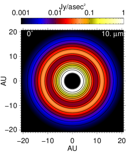
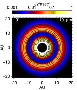
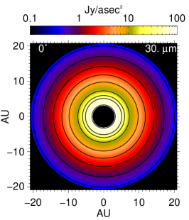
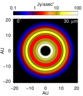
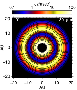
Figure 7.— Simulated images of disks from JC models with and without gaps at 1 (top), 10 (middle), and 30 (bottom) microns. The left, center, and right images in each row show disks with 0, 70, and 200 M_⊕ planets, respectively. The contours are spaced at intervals of factors of two in brightness, and the colors trace brightness according to the displayed color bars.

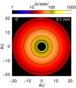
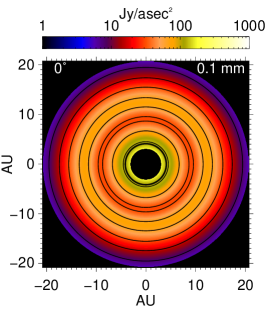
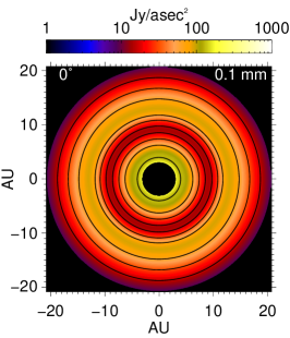
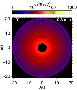
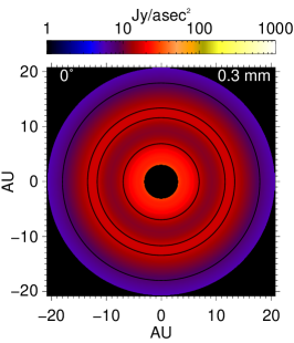
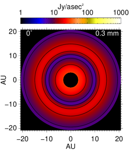
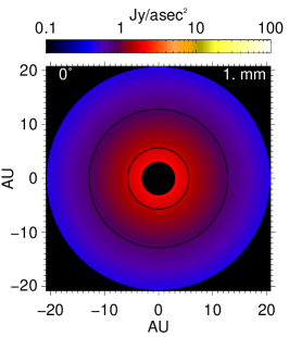
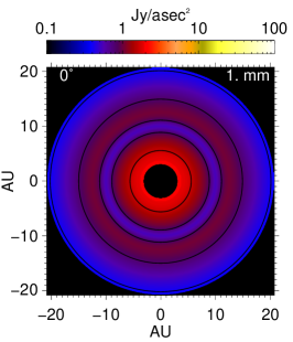
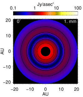
Figure 8.— Same as Figure 7, but at 0.1 (top), 0.3 (middle), and 1 (bottom) mm.

In Figures 7 and 8, we show synthetic images of face-on disks without and with gaps at wavelengths from 1 $\mu$m to 1 mm, as indicated. The star is omitted in each image, but its brightness is that of of a 4280 K blackbody with radius $2.6\,R_{\odot}$. Although the apparent brightness varies as the inverse square of the distance, the surface brightness in Jy/asec² is distance-independent.

The top row in Figure 7 shows the scattered light images of the disks at 1 $\mu$m. The 3 $\mu$m image is very similar to this one, just scaled to the stellar brightness at 3 $\mu$m and modified by the albedo according to Eq. (8). The stellar brightness at 1 $\mu$m at a distance of 140 pc is 0.79 Jy. The shadow in the gap and the brightening outward of the gap are quite apparent. The puffing-up of the outer edge of the gap also creates a further shadowing of the disk beyond the gap. This disk self-shadowing is also evident at longer wavelengths, resulting from cooling in the shadow. Because the disk is not well-modeled outside 20 AU, it is unclear whether or not the full extent of the disk beyond the gap rim is shadowed or not.

The middle row in Figure 7 shows simulated images of the disks at 10 $\mu$m, where the stellar brightness is 0.055 Jy at a distance of 140 pc. In the inner, warm region of the disk, the brightness is dominated by thermal emission from the disk surface. The surface brightness profile is steepest at 10 $\mu$m because the outer disk is too cold to emit efficiently. At about 10 AU and beyond, the brightness profile becomes dominated by scattered light. Both shadowing of scattered light and cooling of the disk surface contribute to the imaged gap structure.

The bottom row in Figure 7 shows the thermal emission from the surface of the disk at 30 $\mu$m. The stellar brightness at this wavelength at a distance of 140 pc is 0.0068 Jy. As with the 10 $\mu$m image, the radial falloff in surface brightness reflects the radial temperature gradient at the disk surface. The gap contrast is highest at 30 microns. This is because the surface temperatures of the disk are $\sim 100$ K, where the blackbody peak is 30 microns. Thus, observations at 30 microns will be the most sensitive to temperature perturbations at the surface of the disk. At shorter wavelengths, the gap contrast is driven by shadowing and illumination at the surface rather than actual temperature changes.

In Figure 8, the top, middle and bottom rows show thermal continuum emission at 0.1, 0.3, and 1 mm, respectively. At these wavelengths, the stellar emission is negligible. The disk becomes more optically thin toward longer wavelengths, so the different wavelengths probe different layers in the disk as well as different temperature regimes. In contrast to the dimple images calculated in JC09, the gaps are still apparent at 1 mm wavelengths because the shadowing effect in the gap is on a much larger scale than the localized dimple. Thus, searching for gaps in disks with ALMA is a promising way of finding planets in during the planet formation epoch.

One might expect that the shadow produced by the gap is offset by the brightened outer edge of the gap, creating a net zero effect on the spectral energy distribution (SED). Because the simulated region is limited in radius, a full SED cannot be produced for the entire disk, as any emission from interior to 4 AU or exterior to 20 AU will be omitted. Nevertheless, we can assess how a gap in a disk changes the SED by integrating over the face on disk images. We approximate the contribution from the inner 4 AU by assuming that the brightness profile goes as $r^{-1}$, is normalized to the brightness at 4 AU for the gapless disk, and is unaffected by the presence of the gap. The star’s emission is approximated as a blackbody of 4280 K and radius 2.6 $R_{\odot}$.

Figure 9.— SEDs of face-on disks with and without gaps from JC models. The SEDs are calculated by summing the total thermal emission over the simulated disks. Top: the disk integrated spectrum of a disk without a gap is plotted as a solid line, while the disks with gaps carved by 70 and 200 $M_{\earth}$ planets are plotted as dotted and dashed lines, respectively. The dot-dashed line shows the stellar photosphere. Bottom: the difference between the gapped disk models and the gap-less disk are plotted in magnitudes. The 70 and 200 $M_{\earth}$ models are shown as dotted and dashed lines, respectively. The maximum deviation from the gapless model occurs at around $\sim 40\,\mu$m, corresponding to the peak of emission for temperature of the disk surface at the gap radius.

In Figure 9, we show the resulting SEDs assuming that the system is at a distance of 140 pc. Since the radiative transfer calculation includes only the annulus lying 3 to 20 AU from the star, the flux approaches that of the whole disk only at wavelengths from 10 to 100 microns, where the annulus emits most strongly. Nevertheless, the difference in fluxes should be representative. The upper panel shows that the gapped SEDs (dotted/dashed line for 70/200 $M_{\oplus}$) are generally brighter than the gapless SED (solid line), particularly at around $30-40\,\mu$m, corresponding to the peak in thermal emission from the disk surface at the gap radius.

The lower panel of Figure 9 shows the difference between gapped and gapless SEDs in magnitudes, with negative values being brighter. These magnitude differences should be interpreted as upper limits on the amount of brightening that can occur, because emission from the outer disk beyond 20 AU has been omitted, and this disk contribution may swamp out the relative differences. Shortward of 10 $\mu$m, stellar flux (dot-dashed line) dominates the SED so the disk contribution is negligible. Beyond the submillimeter regime, emission from the outer disk becomes increasingly important, so the effect of the gap is relatively less than that shown. At best, a 70 (200) $M_{\earth}$ planet increases the brightness of the disk by 0.15 (0.3) mag at 44 (40) $\mu$m, or by 15 (32) %. Beyond about 0.7 mm, the $\Delta$mag becomes positive for the 200 $M_{\earth}$ gap, indicating that there is more dimming than brightening at radio wavelengths. Since the maximum grain size assumed for calculation of the opacities was 1 mm, this is likely because at wavelengths longer than the maximum grain size in disks, the brightness is more representative of the dust distribution in the disk rather than the temperature.

In general, the conclusion is that the brightened outer rim of the gap more than compensates for the lack of emission in the gap trough. The reason for this is the greater amount of heating that occurs on the outer shoulder of the gap, as described in §4.1. Moreover, the contribution to the brightening is amplified because the surface area of the outer rim is greater than the surface area of the gap shadow. However, the contribution of the gap to the SED is subtle, and not easily distinguished from a more massive disk. The SED alone cannot be used to identify a partially cleared gap.

5. Discussion

In JC08, we carried out similar calculations on local perturbations to the disk caused by less massive planets than the gap producing ones modeled in the present work. Since gaps are much larger in physical scale, they produce both a more significant temperature perturbation on the disk and a larger footprint on the disk itself. Thus, planets that produce the gaps modeled in this paper are very likely to be observable, whereas the much more subtle perturbations modeled in JC08 are much harder to observe. Imaging is necessary for detecting these gaps, since the effects are too subtle to identify in the SED alone, as described in §4.2.

The width of the gaps modeled here are on the order of a few AU. If we assume that we need a resolution equivialent to 1-2 AU, then if the disk is at the distance of Taurus, 140 pc, then the angular resolution required would be 0″.01, independent of wavelength. Scattered light observations face the challenge of suppressing the starlight to a small enough working angle to observe the gap, in addition to the angular resolution challenge. ALMA should have sufficient angular resolution to resolve these gaps, but the question them becomes whether or not it will have sufficient sensitivity given the long baselines and sparse $u-v$ coverage required. The size of the gap scales with distance, so a gap at 100 AU would be resolvable with 0″.1 resolution.

We have only modeled gaps at 10 AU in this present work, but we can make some extrapolations to how gaps at other distances in the disk would behave. The same planet mass opens a smaller gap at larger radii because the disk scale height increases faster than the Hill radius of the planet. Thus, the temperature variations would be relatively smaller as the planet is moved further out. On the other hand, gaps created by planets at larger radii should be more easily detectable because gap widths scale with distance, relaxing the angular resolution requirement, and the inner working angle is larger. For interferometers, sensitivity also improves with smaller baselines. We found that the greatest gap contrast was seen at the blackbody peak associated with the temperature of the surface of the disk. At 10 AU, the surface temperature is around 100 K, so the wavelength of greatest contrast is 30 microns. The surface temperature is driven by stellar irradiation, so it should vary roughly as $r^{-1/2}$. This means that to some extent, the wavelength of observation may be tuned to the planet’s orbital radius.

6. Conclusions

We have calculated the thermal effects of gap-opening by planets in protoplanetary disks. The thermal feedback leads to depression of gap troughs and puffing of gap walls, enhancing the observability of gaps carved by planets forming in disks. Planets less than one tenth of the critical gap-opening mass, or 10 M_⊕ at 10 AU, do not create significant gaps in disks. However, a modest gap of only 50%, created by a planet $\sim 10\%$ of the viscous gap-opening mass or 70 M_⊕ at 10 AU, can induce a significant perturbation to the temperature profile of a protoplanetary disk. These gaps are observable in scattered light and thermal emission.

The ability to determine the masses of planets in disks, together with the age of the disks and the locations of gaps, puts vital observational constraints on the time scales of planet formation. If we find that massive planets form early, this might indicate that giant planets form via gravitational instability, which is much faster than the competing paradigm of core accretion. On the other hand, if we only see gap-forming planets at late ages, this might indicate that core accretion is the dominant process. Upper limits on the luminosity of a planet embedded in the disk will determine whether giant planet form more like brown dwarfs with a hot start (Baraffe et al., 2003) or more quiescently with a cold start (Marley et al., 2007).

Temperature variations in the disk produced by shadowing and illumination can have profound effects on the forming planets. We address the consequences for Type I migration in a future paper. These temperature perturbations can also affect the condensation and sublimation of volatiles. Planetesimals just interior to the gap may become enriched in frozen volatiles, while those just outside the gap might become depleted in volatiles via the cold finger effect (Stevenson & Lunine, 1988). This can affect the overall distribution of volatiles in the protoplanetary disk, shift the snow line, and lead to enhanced planet formation in the volatile enriched regions.

Topics for future work include carrying out radiative transfer modeling in a similar way on three-dimensional hydrodynamic simulations of gap-clearing by planets rather than relying on a simple analytic model. This would allow us to capture non-axisymmetric gap characteristics, particularly the region immediately around the planet itself. Our methods can also be applied to the inner walls of fully-cleared inner cavities in transitional disks. If the inner walls are sufficiently puffed up, they can shadow the outer disk and create flat radial surface brightness profiles seen in some disks (Grady et al., 2005). Polarized intensity images are a promising way to resolve protoplanetary disks (e.g.  Oppenheimer et al., 2008), but geometrical effects make these images difficult to interpret (e.g.  Jang-Condell & Kuchner, 2010; Perrin et al., 2009). In a forthcoming paper, we will address how inclination and polarization affects images of disks with and without gaps.

References

- Ayliffe & Bate (2009) Ayliffe, B. A. & Bate, M. R. 2009, MNRAS, 393, 49
- Baraffe et al. (2003) Baraffe, I., Chabrier, G., Barman, T. S., Allard, F., & Hauschildt, P. H. 2003, A&A, 402, 701
- Bate et al. (2003) Bate, M. R., Lubow, S. H., Ogilvie, G. I., & Miller, K. A. 2003, MNRAS, 341, 213
- Bjorkman & Wood (2001) Bjorkman, J. E. & Wood, K. 2001, ApJ, 554, 615
- Crida & Morbidelli (2007) Crida, A. & Morbidelli, A. 2007, MNRAS, 377, 1324
- Crida et al. (2006) Crida, A., Morbidelli, A., & Masset, F. 2006, Icarus, 181, 587
- D’Alessio et al. (2001) D’Alessio, P., Calvet, N., & Hartmann, L. 2001, ApJ, 553, 321
- D’Alessio et al. (1998) D’Alessio, P., Canto, J., Calvet, N., & Lizano, S. 1998, ApJ, 500, 411
- de Val-Borro et al. (2006) de Val-Borro, M., Edgar, R. G., Artymowicz, P., Ciecielag, P., Cresswell, P., D’Angelo, G., Delgado-Donate, E. J., Dirksen, G., Fromang, S., Gawryszczak, A., Klahr, H., Kley, W., Lyra, W., Masset, F., Mellema, G., Nelson, R. P., Paardekooper, S., Peplinski, A., Pierens, A., Plewa, T., Rice, K., Schäfer, C., & Speith, R. 2006, MNRAS, 370, 529
- Dullemond & Dominik (2004) Dullemond, C. P. & Dominik, C. 2004, A&A, 417, 159
- Edgar & Quillen (2008) Edgar, R. G. & Quillen, A. C. 2008, MNRAS, 387, 387
- Grady et al. (2005) Grady, C. A., Woodgate, B. E., Bowers, C. W., Gull, T. R., Sitko, M. L., Carpenter, W. J., Lynch, D. K., Russell, R. W., Perry, R. B., Williger, G. M., Roberge, A., Bouret, J., & Sahu, M. 2005, ApJ, 630, 958
- Jang-Condell (2008) Jang-Condell, H. 2008, ApJ, 679, 797
- Jang-Condell (2009) —. 2009, ApJ, 700, 820
- Jang-Condell & Boss (2007) Jang-Condell, H. & Boss, A. P. 2007, ApJ, 659, L169
- Jang-Condell & Kuchner (2010) Jang-Condell, H. & Kuchner, M. J. 2010, ApJ, 714, L142
- Jang-Condell & Sasselov (2003) Jang-Condell, H. & Sasselov, D. D. 2003, ApJ, 593, 1116
- Jang-Condell & Sasselov (2004) —. 2004, ApJ, 608, 497
- Lucy (1999) Lucy, L. B. 1999, A&A, 344, 282
- Marley et al. (2007) Marley, M. S., Fortney, J. J., Hubickyj, O., Bodenheimer, P., & Lissauer, J. J. 2007, ApJ, 655, 541
- Mulders et al. (2010) Mulders, G. D., Dominik, C., & Min, M. 2010, A&A, 512, A11+
- Oppenheimer et al. (2008) Oppenheimer, B. R., Brenner, D., Hinkley, S., Zimmerman, N., Sivaramakrishnan, A., Soummer, R., Kuhn, J., Graham, J. R., Perrin, M., Lloyd, J. P., Roberts, Jr., L. C., & Harrington, D. M. 2008, ApJ, 679, 1574
- Paardekooper & Papaloizou (2008) Paardekooper, S. & Papaloizou, J. C. B. 2008, A&A, 485, 877
- Perrin et al. (2009) Perrin, M. D., Schneider, G., Duchene, G., Pinte, C., Grady, C. A., Wisniewski, J. P., & Hines, D. C. 2009, ApJ, 707, L132
- Pinte et al. (2006) Pinte, C., Ménard, F., Duchêne, G., & Bastien, P. 2006, A&A, 459, 797
- Pinte et al. (2008) Pinte, C., Padgett, D. L., Ménard, F., Stapelfeldt, K. R., Schneider, G., Olofsson, J., Panić, O., Augereau, J. C., Duchêne, G., Krist, J., Pontoppidan, K., Perrin, M. D., Grady, C. A., Kessler-Silacci, J., van Dishoeck, E. F., Lommen, D., Silverstone, M., Hines, D. C., Wolf, S., Blake, G. A., Henning, T., & Stecklum, B. 2008, A&A, 489, 633
- Rybicki & Lightman (1979) Rybicki, G. B. & Lightman, A. P. 1979, Radiative processes in astrophysics (New York, Wiley-Interscience)
- Shakura & Sunyaev (1973) Shakura, N. I. & Sunyaev, R. A. 1973, A&A, 24, 337
- Siess et al. (2000) Siess, L., Dufour, E., & Forestini, M. 2000, A&A, 358, 593
- Stevenson & Lunine (1988) Stevenson, D. J. & Lunine, J. I. 1988, Icarus, 75, 146
- Tannirkulam et al. (2008) Tannirkulam, A., Monnier, J. D., Harries, T. J., Millan-Gabet, R., Zhu, Z., Pedretti, E., Ireland, M., Tuthill, P., ten Brummelaar, T., McAlister, H., Farrington, C., Goldfinger, P. J., Sturmann, J., Sturmann, L., & Turner, N. 2008, ApJ, 689, 513
- Thalmann et al. (2010) Thalmann, C., Grady, C. A., Goto, M., Wisniewski, J. P., Janson, M., Henning, T., Fukagawa, M., Honda, M., Mulders, G. D., Min, M., Moro-Martín, A., McElwain, M. W., Hodapp, K. W., Carson, J., Abe, L., Brandner, W., Egner, S., Feldt, M., Fukue, T., Golota, T., Guyon, O., Hashimoto, J., Hayano, Y., Hayashi, M., Hayashi, S., Ishii, M., Kandori, R., Knapp, G. R., Kudo, T., Kusakabe, N., Kuzuhara, M., Matsuo, T., Miyama, S., Morino, J., Nishimura, T., Pyo, T., Serabyn, E., Shibai, H., Suto, H., Suzuki, R., Takami, M., Takato, N., Terada, H., Tomono, D., Turner, E. L., Watanabe, M., Yamada, T., Takami, H., Usuda, T., & Tamura, M. 2010, ApJ, 718, L87
- Turner et al. (2011) Turner, N. J., Choukroun, M., Castillo-Rogez, J., & Bryden, G. 2011, ApJ, in press, astro-ph 1110.4166
- Varnière et al. (2006) Varnière, P., Bjorkman, J. E., Frank, A., Quillen, A. C., Carciofi, A. C., Whitney, B. A., & Wood, K. 2006, ApJ, 637, L125
- Varnière et al. (2004) Varnière, P., Quillen, A. C., & Frank, A. 2004, ApJ, 612, 1152
- Walker et al. (2004) Walker, C., Wood, K., Lada, C. J., Robitaille, T., Bjorkman, J. E., & Whitney, B. 2004, MNRAS, 351, 607
- Wolf et al. (2002) Wolf, S., Gueth, F., Henning, T., & Kley, W. 2002, ApJ, 566, L97