Local Magnetization in the Boundary Ising Chain at Finite Temperature

Abstract

We study the local magnetization in the 2-D Ising model at its critical temperature on a semi-infinite cylinder geometry, and with a nonzero magnetic field $h$ applied at the circular boundary of circumference $\beta$. This model is equivalent to the semi-infinite quantum critical 1-D transverse field Ising model at temperature $T\propto\beta^{-1}$, with a symmetry-breaking field $\propto h$ applied at the point boundary. Using conformal field theory methods we obtain the full scaling function for the local magnetization analytically in the continuum limit, thereby refining the previous results of Leclair, Lesage and Saleur in Ref. Lesage et al., 1996. The validity of our result as the continuum limit of the 1-D lattice model is confirmed numerically, exploiting a modified Jordan-Wigner representation. Applications of the result are discussed.

I Introduction

The Ising model is a classic paradigm of statistical mechanics, and continues to find powerful application in diverse areas of modern physics.Len ; mcc (a, b) It also reveals unique and generic universal behavior associated with boundaries. bar ; Cardy (1984, 1989) In its quantum 1-D chain version, the critical boundary Ising model (BIM) reads

$$H=-\sum_{i=0}^{\infty}[\sigma^{z}_{i}\sigma^{z}_{i+1}+\sigma^{x}_{i}]-h_{B}\sigma^{z}_{0}.$$ (1)

The uniform field along $x$ is fixed such that the bulk system is at the critical point between Ising order and the disordered phase. The symmetry $\sigma^{z}\leftrightarrow-\sigma^{z}$ is broken when a finite magnetic field $h_{B}\neq 0$ is applied at the point boundary. Such a boundary field cannot lead to a finite bulk magnetization. Importantly however, it does cause a renormalization group flow from a free boundary condition $h_{B}=0$ to a fixed boundary condition $h_{B}\to\pm\infty$.

The renormalization group flow associated with this BIM has been shown to be at the heart of boundary critical phenomena occurring in a surprising variety of low-dimensional correlated electron systems, such as Luttinger liquids containing an impurity,Lesage et al. (1996) coupled bulk and edge states in non-abelian fractional quantum Hall states,ros ; Bis as well as quantum dots near the two impurity KondoCFT ; Sel or the two channel KondoSela et al. (2011); Mitchell et al. (2011) critical points.

In the continuum, the BIM is in fact integrable,gho both in the massless bulk critical case, and also in the massive regime away from the critical point. Certain correlation functions can then be calculated exactly using Form Factor methods;kon ; sch although in the bulk critical case relevant to Eq. (1), many important quantities cannot be easily obtained due to the proliferation of many-particle excitations. On the other hand, Chatterjee and Zamolodchikovcz (CZ) showed that conformal field theory imposes linear differential equations which fully determine correlation functions in this limit. Of course, conformal field theory has been used previously for systems with conformal-invariant boundary conditions.Cardy (1984, 1989) The remarkable feature of the result of CZ is that the correlation functions are still determined by differential equations even for non-conformal invariant boundary conditions obtained at finite boundary field.

The method of CZ was applied to the calculation of magnetization as a function of distance from the boundary, $x$. On the semi-infinite plane, equivalent to the quantum 1-D model, Eq. (1), at zero temperature, their result readscz

$$\langle\sigma(x)\rangle_{h}=2^{13/8}\sqrt{\pi}hx^{3/8}\Psi(1/2,1;8\pi h^{2}x),$$ (2)

where $\Psi$ is a degenerate hypergeometric function. Here $\langle\sigma(x)\rangle$ has the standard field-theory normalization, which we emphasize is only proportional to $\langle\sigma^{z}_{j}\rangle$ of a particular lattice model, such as Eq. (1). Indeed, $x\propto j$, and $h\propto h_{B}$ provided that $h_{B}\ll 1$. At short distance one thus obtains,

$$\langle\sigma(x)\rangle=-2^{13/8}hx^{3/8}[\ln(x)+\mathcal{O}(1)]+\mathcal{O}(x^{7/8})\qquad\text{for}\leavevmode\nobreak\ x\ll 1,$$ (3)

and at long distances $\langle\sigma(x)\rangle\rightarrow(2/x)^{1/8}$, corresponding exactly to the result for fixed boundary condition, obtained from boundary conformal field theory.car (a) As such, the exact function, Eq. (2), captures the full crossover behavior between two fixed points where conformal invariant boundary conditions do hold.

Since the problem for finite $h$ does not in general possess conformal invariance at the boundary, it is not possible to generalize Eq. (2) to other geometries by means of a simple conformal mapping. However the method of CZ can be applied directly to other geometries, yielding a new set of differential equations (this was demonstrated explicitly for the 2-D disk geometry by CZcz ). Similarly, Leclair, Lesage and SaleurLesage et al. (1996) (LLS) applied the method to the geometry of a semi-infinite cylinder. In the present paper we shall be concerned with this semi-infinite cylinder geometry, whose boundary consists of a circle with circumference $\beta$, at which the boundary field $h$ is applied. This classical 2-D Ising model is equivalent to the quantum chain model Eq. (1) at finite temperature $T\propto\beta^{-1}$ (see e.g. Ref.car, b).

We re-examine the result of LLS for the local magnetization in Sec. II. Whereas those nonperturbative results give the full $x$-dependence of the local magnetization for any $h$ and $\beta$, we find that a more general ansatz for the local magnetization allows for an additional multiplicative factor $f(2\beta h^{2})$. The physical meaning of this missing factor is then explained. The full scaling function for the local magnetization is determined in Sec. III; while the lattice model Eq. (1) is studied directly in Sec. IV. The local magnetization on the lattice is calculated numerically, and the results compared with the refined analytic solution, showing excellent agreement. The paper ends with a short summary, where implications and applications of the results are discussed.

II Refinement of earlier results

LLS considered a classical Ising model on the half-cylinder in the continuum limit.Lesage et al. (1996) They calculated the local magnetization as a function of the distance $x$ from the circular boundary of circumference $\beta$, which was conveniently written in the formLesage et al. (1996)

$$\langle\sigma(x)\rangle=\left(\frac{1}{\sinh\frac{2\pi x}{\beta}}\right)^{1/8}g(X),$$ (4)

with $X=(1-\coth\frac{2\pi x}{\beta})/2$ and where $\langle\sigma(x)\rangle$ is independent of $\tau\in(0,\beta)$ due to translation symmetry along the boundary. LLS derived a linear differential equation for $g(X)$, which readsLesage et al. (1996)

$$\left((X-X^{2})\frac{d^{2}}{(dX)^{2}}+\left(1+\frac{\Lambda}{2}-2X\right)\frac{d}{dX}-\frac{1}{4}\right)g(X)=0,$$ (5)

parametrized in terms of $\Lambda=2\beta h^{2}$. Their solution isLesage et al. (1996)

$$\langle\sigma(x)\rangle_{LLS}=\left(\frac{\frac{4\pi}{\beta}}{\sinh\frac{2\pi x}{\beta}}\right)^{1/8}\leavevmode\nobreak\ _{2}F_{1}\left(\frac{1}{2},\frac{1}{2};1+2\beta h^{2},\frac{1-\coth\frac{2\pi x}{\beta}}{2}\right),$$ (6)

where ${}_{2}F_{1}(a,b,c,z)$ is the Gauss hypergeometric function. Below we will use its integral representation

$${}_{2}F_{1}(a,b,c,z)=\frac{\Gamma[c]}{\Gamma[b]\Gamma[c-b]}\int_{0}^{1}dt\frac{t^{b-1}(1-t)^{c-b-1}}{(1-tz)^{a}},$$ (7)

where $\Gamma(y)$ is the gamma function. This result is normalized with an overall constant such that at long distances $\langle\sigma(x)\rangle\to\left(\frac{\frac{4\pi}{\beta}}{\sinh\frac{2\pi x}{\beta}}\right)^{1/8}$ recovers the expected result for fixed boundary conditions (taking $\beta\rightarrow\infty$ then yields $\langle\sigma(x)\rangle\rightarrow(2/x)^{1/8}$, consistent with Ref. car, a).

In this paper we point out that the differential equation Eq. (5) leaves a freedom which goes beyond an overall normalization constant. Unlike the zero-temperature case (corresponding to the semi-infinite plane, $\beta\rightarrow\infty$), here the normalization of Eq. (6) can itself be a scaling function of $\Lambda$. We thus replace Eq. (6) by the more general ansatz,

$$\langle\sigma(x)\rangle_{h,\beta}=f(2\beta h^{2})\times\left(\frac{\frac{4\pi}{\beta}}{\sinh\frac{2\pi x}{\beta}}\right)^{1/8}\leavevmode\nobreak\ _{2}F_{1}\left(\frac{1}{2},\frac{1}{2};1+2\beta h^{2},\frac{1-\coth\frac{2\pi x}{\beta}}{2}\right),$$ (8)

which depends explicitly on the function $f(2\beta h^{2})$, determined in Sec. III, below. Eq. (8) implies $f(\infty)=1$, so that $\langle\sigma(x)\rangle_{h,\beta}$ recovers asymptotically the behavior of the fixed boundary condition fixed point.

We note that the same subtlety occurs with other geometries, as highlighted by CZ in the case of the disk.cz In that case, the additional scale in the problem is the disk radius $R$; and an additional scaling function of $Rh^{2}$ (analogous to our $\Lambda=2\beta h^{2}$) appears in the expression for the local magnetization. As in the present case, this function is not fixed by the linear differential equations.cz

Finally, we comment briefly upon the physical significance of the scaling function $f(2\beta h^{2})$. It describes the dependence on the additional thermal scale influencing the renormalization group flow at $T\neq 0$. In accord with physical expectation, the renormalization group flow is cut off at the external scale given by $\max\{T,x^{-1}\}$. Since $h$ grows under renormalization (and has scaling dimension $1/2$), Cardy (1984, 1989) we should consider two regimes depending on the ratio between this external scale and the field-induced scale $\sim h^{2}$:

$$\max\{T,x^{-1}\} \gg h^{2}:{\rm{\leavevmode\nobreak\ free\leavevmode\nobreak\ boundary\leavevmode\nobreak\ condition}},$$

$$\max\{T,x^{-1}\} \ll h^{2}:{\rm{\leavevmode\nobreak\ fixed\leavevmode\nobreak\ boundary\leavevmode\nobreak\ condition}}.$$ (9)

These regimes are illustrated in Fig. 1. The important consequence following from this is that at finite temperatures, the fixed boundary condition fixed point is not always reached on taking $x\to\infty$. The single scaling function $f(2\beta h^{2})$ thus describes the crossover from free to fixed boundary condition at a given $x$, upon decreasing temperature. Obviously its effect is most apparent at large $x$, since there is no crossover at small $x$. However, as suggested by Fig. 1, the system is always close to the free boundary condition fixed point at small $x$, and this fact will prove useful in determining $f(2\beta h^{2})$, as considered in the next section.

Figure 1: Schematic phase diagram of the BIM as a function of temperature and distance from the boundary. The dashed line denotes the crossover between free and fixed boundary conditions occurring when $\max\{T,x^{-1}\}\sim h^{2}$.

III Determination of the scaling function $f(2\beta h^{2})$

In this section we find the function $f(2\beta h^{2})$ appearing in Eq. (8). Since this function is a scaling function of $\beta h^{2}$ and does not depend on distance $x$, it could in principle be determined at any given $x$. While its influence is most pronounced at large $x$, where the system undergoes a crossover as function of $T$ (see Fig. 1), here we determine $f(2\beta h^{2})$ by exploring the small $x$ behavior, where the system remains close to free boundary condition fixed point. Importantly, the resulting behavior at small $x$ is perturbative in $h$ regardless of $\beta h^{2}$, as shown explicitly below.

First we note that at both large and small $\Lambda$, the short-distance behavior of $\langle\sigma(x)\rangle$ is linear in $h$. As $\Lambda\rightarrow\infty$, one sees this directly from the small $x$ expansion of the exact $T=0$ result of CZ, Eq. (3). In the opposite limit $\Lambda\rightarrow 0$, the behavior is by definition perturbative in $h$, and so the leading correction to magnetization is of course also linear in $h$. In the next subsection, we perform first-order perturbation theory in the boundary field $h$, with respect to the free boundary condition fixed point. The key point is that its short-distance behavior yields precisely Eq. (3), implying that

$$\langle\sigma(x)\rangle_{h,\beta}=-2^{13/8}hx^{3/8}[\ln(x)+\mathcal{O}(1)]+\mathcal{O}(x^{7/8})\qquad\text{for}\leavevmode\nobreak\ x\ll\beta,h^{-2}$$ (10)

holds at short distances $x\ll\beta,h^{-2}$ for any $\Lambda$. Naively one might think that the coefficient of the $x^{3/8}[\ln(x)+\mathcal{O}(1)]$ term could be renormalized by higher orders in $h$. But the scaling form of the problem implies that every power of $h$ is accompanied by a power of $\sqrt{\beta}$ [or $\sqrt{x}$ which gives a subleading $x$ dependence to Eq. (10)]. Such terms diverge as $T\to 0$, and so this renormalization is not consistent with the exact nonperturbative $T=0$ result, Eq. (2), which is well-behaved at short distances, Eq. (3).

Finally, we consider the short distance expansion of our ansatz Eq. (8), which using Eq. (7) is found to be

$$\langle\sigma(x)\rangle_{h,\beta}=-f(2\beta h^{2})\frac{2^{9/8}}{\sqrt{\beta}}\frac{\Gamma[1+2\beta h^{2}]}{\Gamma[\tfrac{1}{2}+2\beta h^{2}]}x^{3/8}[\ln(x)+\mathcal{O}(1)]+\mathcal{O}(x^{7/8})\qquad\text{for}\leavevmode\nobreak\ x\ll 1.$$ (11)

Comparing Eqs. (10) and (11) we now obtain the scaling function

$$f(\Lambda)=\sqrt{\Lambda}\frac{\Gamma[\tfrac{1}{2}+\Lambda]}{\Gamma[1+\Lambda]}.$$ (12)

This function increases monotonically as shown in Fig  2, and has asymptotic limits $f(\Lambda\ll 1)\approx\sqrt{\pi\Lambda}$ and $f(\Lambda\gg 1)\approx 1-\frac{1}{8\Lambda}$.

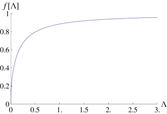
Figure 2: Plot of Eq. (12).

We note that a similar perturbative method was used by CZ to fix the scaling function of $Rh^{2}$ for the disk geometry.cz

III.1 Perturbation theory in the boundary field $h$

In this subsection we show that the form of Eq. (10) indeed follows from perturbation theory around the free boundary condition fixed point. We obtain the full $x/\beta$ dependence of the magnetization at small $h$, recovering perturbatively the $\Lambda\rightarrow 0$ limit of Eq. (8).

The continuum limit of the critical classical 2-D Ising model is described by a $c=1/2$ conformal field theory, which admits a Lagrangian formulation in terms of the free massless Majorana Fermi field ($\psi$,$\bar{\psi}$), with the action

$$S_{0}=\frac{1}{2\pi}\int d^{2}z[\psi\partial_{\bar{z}}\psi+\bar{\psi}\partial_{z}\bar{\psi}].$$ (13)

Here $(z,\bar{z})=(\tau+ix,\tau-ix)$ are complex coordinates and $d^{2}z=d\tau dx$. In the presence of a boundary $\mathcal{B}$ with a magnetic field $h$, the action can be decomposed into a bulk part and a boundary part,

$$S=\frac{1}{2\pi}\int_{\mathcal{D}}d^{2}z[\psi\partial_{\bar{z}}\psi+\bar{\psi}\partial_{z}\bar{\psi}]+h\int_{\mathcal{B}}\sigma_{B}.$$ (14)

The boundary operator $\sigma_{B}$ was identified in Refs. Cardy, 1984, 1989 with a dimension $1/2$ operator $\sigma_{B}(\tau)\sim\psi(\tau,x=0)$, associated with the fermion field at the boundary. In our case $\mathcal{B}=\partial\mathcal{D}$ is a circle parametrized by $\tau\in[0,\beta]$ and $\mathcal{D}$ is the semi-infinite cylinder. Following Cardy’s method of images Cardy (1984) the one point function of the magnetization is $\sigma(z_{1},z_{2})=\langle\sigma_{L}(z_{1})\sigma_{L}(z_{2})\rangle$, where $\sigma_{L}(z)$ is a dimension $1/16$ left moving field living in the geometry of the infinite cylinder. We then obtain conformal invariant boundary conditions, with the ‘boundary’ at $x=0$. The boundary field $h$ is now considered as a perturbation to the free boundary condition fixed point. To first order in $h$,

$$\sigma^{(1)}(z_{1},z_{2})=h\int_{0}^{\beta}d\tau\langle\sigma(z_{1})\sigma_{B}(0,\tau)\sigma(z_{2})\rangle.$$ (15)

The 3-point function appearing in the integrand is fully determined by conformal invariance, and one obtains up to a normalization constant $N$

$$\sigma^{(1)}(z_{1},z_{2})=hN\left(\frac{\sin\frac{\pi}{\beta}(z_{1}-z_{2})}{\frac{\pi}{\beta}}\right)^{3/8}\int_{0}^{\beta}d\tau\leavevmode\nobreak\ \frac{\frac{\pi}{\beta}}{\left[\sin\left(\frac{\pi}{\beta}(\tau-z_{1})\right)\sin\left(\frac{\pi}{\beta}(\tau-z_{2})\right)\right]^{1/2}}.$$ (16)

The physical magnetization is obtained by setting $\langle\sigma(x)\rangle=\langle\sigma(z_{1}=ix,z_{2}=-ix)\rangle$. We now take $z_{1}=ix$, $z_{2}=-ix$ in Eq. 16 and use the trigonometric identity,

$$2\sin\left(\frac{\pi}{\beta}(\tau-z_{1})\right)\sin\left(\frac{\pi}{\beta}(\tau-z_{2})\right)=\cos\left(\frac{2i\pi x}{\beta}\right)-\cos\left(\frac{2\pi\tau}{\beta}\right).$$ (17)

The integral in Eq. (16) then becomes

$$\int_{0}^{2\pi}\frac{d\theta}{\sqrt{\frac{w^{1/2}+w^{-1/2}}{2}-\cos\theta}}=\frac{2\pi}{\sqrt{\sinh\frac{2\pi x}{\beta}}}\leavevmode\nobreak\ _{2}F_{1}\left(\frac{1}{2},\frac{1}{2};1,\frac{1-\coth\frac{2\pi x}{\beta}}{2}\right),$$ (18)

in terms of $w=e^{-4\pi x/\beta}$ and $\theta=2\pi\tau/\beta$. The constant $N$ was carefully accounted for by CZ.cz Using this and Eq. (18), first-order perturbation theory in the boundary field $h$ yields

$$\langle\sigma(x)\rangle_{\beta}^{(1)}=h\sqrt{2\pi\beta}\left(\frac{\frac{4\pi}{\beta}}{\sinh\frac{2\pi x}{\beta}}\right)^{1/8}\leavevmode\nobreak\ _{2}F_{1}\left(\frac{1}{2},\frac{1}{2};1,\frac{1-\coth\frac{2\pi x}{\beta}}{2}\right)+\mathcal{O}(h^{2}).$$ (19)

It is interesting to compare this with the full result of LLS, Eq. (6). At small $h$, both carry the same $x/\beta$ dependence; however LLS miss the overall linear dependence on $h$, accounted for by the function $f(2\beta h^{2})$ in Eq. (8).

The short distance behavior of Eq. (19) is precisely Eq. (10).

IV Demonstration with numerical solution

In this section we demonstrate the validity of Eq. (8) as the continuum limit of the lattice magnetization

$$\langle\sigma(j,h_{B},T)\rangle\equiv\frac{{\rm{Tr}}(e^{-H/T}\sigma^{z}_{j})}{{\rm{Tr}}(e^{-H/T})},$$ (20)

where $H$ is the Hamiltonian of the lattice model, Eq. (1). The quantum boundary Ising chain can be solved by applying a Jordan-Wigner transformation, which yields a quadratic fermionic Hamiltonian. The magnetization is nonlocal in terms of these fermions: calculation of $\sigma(j,h_{B},T)\rangle$ is then equivalent to evaluation of the determinant of a matrix whose elements are fermionic correlation functions.Sachdev (1999) We construct these analytically, but ultimately evaluate them numerically. Details of this calculation follow in Sec. IV.1. Here we pre-empt that discussion and present our numerical results, comparing to the refined exact expression, Eq. (8).

The continuum limit expression Eq. (8) admits the scaling form

$$\langle\sigma(x,h,T)\rangle=T^{1/8}\mathcal{F}[x/\beta,2\beta h^{2}].$$ (21)

For this function to be a continuum limit of the lattice magnetization, there should exist nonuniversal constants $c,c_{x},c_{h}$ such that

$$\langle\sigma(j,h_{B},T)\rangle=cT^{1/8}\mathcal{F}[c_{x}j/\beta,2c_{h}\beta h_{B}^{2}]$$ (22)

is satisfied for all $j,h_{B}$ and $T$, as long as distances are large compared to the lattice constant, $j\gg 1$, and the energy scales $h_{B}$ and $T$ are small compared to the lattice cutoff scale, $h_{B},T\ll 1$.

The constant $c_{x}$ is related to the velocity $v$ of bulk excitations via $c_{x}=v^{-1}$. This follows from the requirement that the exponential decay at long distances $j\gg\beta$ is given by Gia $\langle\sigma(x=j)\rangle=\langle\sigma(z_{1}=ix)\sigma(z_{2}=-ix)\rangle\to e^{-(2\nu)\pi(2j)/(v\beta)}$, with $\nu=1/16$ being the scaling dimension of the chiral $\sigma$ field. In our model we obtain $c_{x}=1/2$ exactly. $c$ is an overall factor relating the lattice magnetization to the field theory one, and $c_{h}$ relates the (squared) boundary field, $h_{B}$, in the lattice model to $h$ appearing in the continuum action, Eq. (14). We determine $c$ and $c_{h}$ by demanding that the ratio

$$\frac{\langle\sigma(j,h_{B},T)\rangle}{cT^{1/8}\mathcal{F}[c_{x}j/\beta,2c_{h}\beta h_{B}^{2}]}$$ (23)

is equal to unity for all $h_{B}$. The best fit from our numerical data was obtained for $c_{h}\simeq 0.161$ and $c\simeq 0.729$.

As shown in Fig. 3, we obtain essentially perfect agreement between numerical calculations and field theoretical predictions for the magnetization as a full function of distance, over a wide range of $2h^{2}/T=2c_{h}h_{B}^{2}/T$.

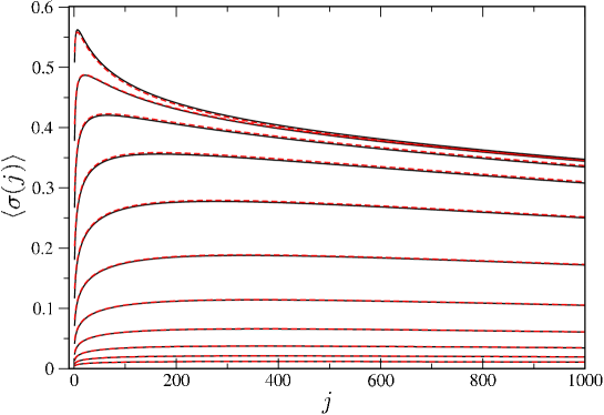
Figure 3: Comparison of analytical result using Eq. (8) (full lines) and numerical results (dashed lines) for fixed temperature $T=0.5\leavevmode\nobreak\ 10^{-3}$ and varying boundary field $h_{B}=10^{-3+n/4}/\sqrt{2}$, $n=0,1,...,10$ increasing from bottom to top [explicitly $h_{B}=0.000707,0.00125,0.00223,0.00397,0.00707,0.0125,0.0223,0.0397,0.0707,0.125,0.223$].

Fig. 3 should be seen as confirmation that the $x$ dependence of the magnetization is described by the LLS result, Eq. (6). However, the full dependence on $h$, $x$ and $T$ — capturing the evolution from the $T\ll h^{2}$ result of CZ, Eq. (2), to the perturbative $T\gg h^{2}$ result, Eq. (19) — is only recovered on inclusion of the factor $f(2\beta h^{2})$ appearing in Eq. (8).

IV.1 Modified Jordan-Wigner transformation and construction of the magnetization determinant

We now describe the calculation of the magnetization using a fermionic representation of the transverse field quantum Ising chain, Eq. (1). We start from a finite lattice with $L$ sites,

$$H_{L}=-\sum_{i=0}^{L-2}\sigma^{z}_{i}\sigma^{z}_{i+1}-\sum_{i=0}^{L-1}\sigma^{x}_{i}-h_{B}\sigma^{z}_{0},$$ (24)

with boundary field $h_{B}$ at site $j=0$; and with free boundary conditions at site $j=L-1$. Ultimately we will take the $L\to\infty$ limit to avoid finite size effects.

Consider first the usual Jordan-Wigner representation of the Pauli matrices $\tau_{j}$ $(j=0,...,L-1)$,

$$\tau^{x}_{j} = i\gamma_{B,j}\gamma_{A,j},$$

$$\tau^{z}_{j} = -\left(\prod_{\ell=0}^{j-1}i\gamma_{A,\ell}\gamma_{B,\ell}\right)\gamma_{B,j},$$ (25)

in terms of self-Hermitian (Majorana) lattice fermions $\gamma_{A(B),j}$, satisfying $\{\gamma_{A,j},\gamma_{A,j^{\prime}}\}=2\delta_{jj^{\prime}}$, $\{\gamma_{B,j},\gamma_{B,j^{\prime}}\}=2\delta_{jj^{\prime}}$, $\{\gamma_{A,j},\gamma_{B,j^{\prime}}\}=0$. Here, $\tau^{y}_{j}$ can be obtained from $i\tau^{y}_{j}=\tau^{z}_{j}\tau^{x}_{j}$. Employing this representation for Eq. (24), one obtains a linear term involving a single fermionic operator representing the boundary spin operator, $\tau^{z}_{0}=-\gamma_{B,0}$. This proves to be inconvenient in the following, and so we use a modified fermionic representation of the spins to eliminate this linear term from the Hamiltonian. Specifically, we introduce an extra boundary Majorana fermion $\gamma$ (with $\gamma^{2}=1$), which anticommutes with all other fermions $\gamma_{A,j}$ and $\gamma_{B,j}$. It can be checked that, if $[\tau_{j}^{a},\tau_{j^{\prime}}^{b}]=2i\epsilon^{abc}\delta_{jj^{\prime}}\tau^{c}_{j}$, then $\{\sigma_{j}^{x},\sigma_{j}^{y},\sigma_{j}^{z}\}\equiv\{\sigma_{j}^{x},i\gamma\sigma_{j}^{y},i\gamma\sigma_{j}^{z}\}$ also satisfy $[\sigma_{j}^{a},\sigma_{j^{\prime}}^{b}]=2i\epsilon^{abc}\delta_{jj^{\prime}}\sigma^{c}_{j}$. Thus we work with the modified Jordan-Wigner representation

$$\sigma^{x}_{j} = i\gamma_{B,j}\gamma_{A,j},$$

$$\sigma^{z}_{j} = -i\gamma\left(\prod_{\ell=0}^{j-1}i\gamma_{A,\ell}\gamma_{B,\ell}\right)\gamma_{B,j}.$$ (26)

This is formally equivalent to embedding the spins in a larger Hilbert space. The model Eq. (24) now becomes a tight binding model of Majorana fermions, containing only quadratic terms:

$$H_{L}=\sum_{j=0}^{L-2}i\gamma_{A,j}\gamma_{B,j+1}+\sum_{j=0}^{L-1}i\gamma_{A,j}\gamma_{B,j}+h_{B}i\gamma\gamma_{B,0}.$$ (27)

The model can be straightforwardly diagonalized by introducing the fermionic modes

$$A_{n}=\frac{1}{2}\sum_{j=0}^{L-1}\left(g_{n}(j+\tfrac{1}{2})\gamma_{A,j}+ig_{n}(j)\gamma_{B,j}\right),\leavevmode\nobreak\ \leavevmode\nobreak\ \leavevmode\nobreak\ (n=1,2,...,L)$$ (28)

with

$$g_{n}(j)=\sqrt{\frac{2}{L+\tfrac{1}{2}}}\sin\left(\frac{\pi n}{L+\tfrac{1}{2}}(j+\tfrac{1}{2})\right)$$ (29)

satisfying the completeness relation $\sum_{n=1}^{L}g_{n}(j)g_{n}(j^{\prime})=\sum_{n=1}^{L}g_{n}(j+\tfrac{1}{2})g_{n}(j^{\prime}+\tfrac{1}{2})=\delta_{jj^{\prime}}$. This gives $\{A_{n},A_{n^{\prime}}\}=\delta_{n,n^{\prime}}$, and

$$\gamma_{A,j} = \sum_{n=1}^{L}g_{n}(j+\tfrac{1}{2})(A_{n}+A_{n}^{\dagger}),$$

$$i\gamma_{B,j} = \sum_{n=1}^{L}g_{n}(j)(A_{n}-A_{n}^{\dagger}).$$ (30)

The Hamiltonian thus becomes,

$$H_{L}=\sum_{n=1}^{L}E_{n}A_{n}^{\dagger}A_{n}+h_{B}\sum_{n=1}^{L}g_{n}(0)\gamma(A_{n}-A_{n}^{\dagger}),$$ (31)

with $E_{n}=4\cos\frac{\pi n}{2L+1}$, which consists of a band of fermionic levels coupled to a Majorana impurity.

Using Eq. (IV.1) the magnetization is given by

$$\langle\sigma^{z}_{j}\rangle=-i^{j+1}\langle\gamma\leavevmode\nobreak\ \gamma_{B,0}\gamma_{A,0}\gamma_{B,1}\gamma_{A,1}...\gamma_{B,j-1}\gamma_{A,j-1}\gamma_{B,j}\rangle.$$ (32)

One proceeds using Wicks theorem,Sachdev (1999) applicable for the quadratic Hamiltonian Eq. (31). Due to the bipartite structure in Eq. (27) it follows that $\langle\gamma_{A,j}\gamma_{A,j^{\prime}}\rangle=\langle\gamma\gamma_{A,j^{\prime}}\rangle=\langle\gamma_{B,j}\gamma_{B,j^{\prime}}\rangle=0$. All nonzero contractions, including relative signs, are then captured by the determinant

$$\langle\sigma^{z}_{j}\rangle=-\left|\left(\begin{array}[]{cccc}i\langle\gamma\gamma_{B,0}\rangle&i\langle\gamma\gamma_{B,1}\rangle&\cdots&i\langle\gamma\gamma_{B,j}\rangle\\ i\langle\gamma_{A,0}\gamma_{B,0}\rangle&i\langle\gamma_{A,0}\gamma_{B,1}\rangle&\cdots&i\langle\gamma_{A,0}\gamma_{B,j}\rangle\\ \vdots&\vdots&\ddots&\vdots\\ i\langle\gamma_{A,j-1}\gamma_{B,0}\rangle&i\langle\gamma_{A,j-1}\gamma_{B,1}\rangle&\cdots&i\langle\gamma_{A,j-1}\gamma_{B,j}\rangle\\ \end{array}\right)\right|.$$ (33)

The calculation of the fermionic correlators in Eq. (33) can be done by exact Green function resummation, treating the problem as a noninteracting impurity model.Hewson (1993) In Eq. (31) we have a quasi-continuum of modes labeled by $n$ coupled to a localized impurity state $\gamma$. The Green functions for $n$-modes and for the localized state are defined as

$$\hat{G}_{nn^{\prime}}(\tau) = -\langle\mathcal{T}\left(\begin{array}[]{c}A_{n}(\tau)\\ A_{n}^{\dagger}(\tau)\\ \end{array}\right)\left(\begin{array}[]{cc}A_{n^{\prime}}^{\dagger}&A_{n^{\prime}}\\ \end{array}\right)\rangle,$$ (37)

$$G_{\gamma}(\tau) = -\langle\mathcal{T}\gamma(\tau)\gamma\rangle,$$ (38)

where $O(\tau)=e^{H_{L}\tau}Oe^{-H_{L}\tau}$, and $\mathcal{T}$ is Wick’s time-ordering operator. We now construct a perturbative expansion of the Green functions in $h_{B}$, with $G(i\omega_{m})=\int_{0}^{\beta}d\tau e^{i\omega_{m}\tau}G(\tau)$ in terms of the Matsubara frequencies $\omega_{m}=\pi T(1+2m)$. The zeroth-order Green functions are given by

$$\hat{G}_{nn^{\prime}}^{(0)}(i\omega_{m})=\delta_{nn^{\prime}}\left(\begin{array}[]{cc}i\omega_{m}-E_{n}&0\\ 0&i\omega_{m}+E_{n}\\ \end{array}\right)^{-1},\leavevmode\nobreak\ \leavevmode\nobreak\ \leavevmode\nobreak\ G_{\gamma}^{(0)}(i\omega_{m})=\frac{2}{i\omega_{m}}.$$ (41)

The full impurity Green function can then be written as $G_{\gamma}(i\omega_{m})=[(G_{\gamma}^{(0)}(i\omega_{m}))^{-1}-\Sigma(i\omega_{m})]^{-1}$. Writing the boundary term in the Hamiltonian as $H_{L}|_{h_{B}}=h_{B}\sum_{n=1}^{L}g_{n}(0)\gamma\left(\begin{array}[]{cc}A_{n}^{\dagger}&A_{n}\\ \end{array}\right)\left(\begin{array}[]{c}-1\\ 1\\ \end{array}\right)$, the exact self energy follows as

$$\Sigma(i\omega_{m})=h_{B}^{2}\sum_{n=1}^{L}g^{2}_{n}(0)\left(\begin{array}[]{cc}1&-1\\ \end{array}\right)\hat{G}_{nn}^{(0)}(i\omega_{m})\left(\begin{array}[]{c}1\\ -1\\ \end{array}\right)=-h_{B}^{2}\sum_{n=1}^{L}g^{2}_{n}(0)\frac{2i\omega_{m}}{(\omega_{m})^{2}+E_{n}^{2}}.$$ (45)

We can now calculate the fermionic correlators entering the determinant Eq. (33). With $G(\tau)=T\sum_{\omega_{m}}e^{-i\omega_{m}\tau}G(i\omega_{m})$, the correlators involving the impurity fermion are given by

$$i\langle\gamma\gamma_{B,x}\rangle=i\langle\mathcal{T}\gamma(\tau=0^{+})\gamma_{B,x}\rangle=iT\sum_{\omega_{m}}e^{-i\omega_{m}0^{+}}\langle\gamma\gamma_{B,x}\rangle_{\omega_{m}}$$

$$=T\sum_{\omega_{m}}e^{-i\omega_{m}0^{+}}\sum_{n=1}^{L}g_{n}(x)\langle\gamma(A_{n}-A_{n}^{\dagger})\rangle_{\omega_{m}},$$ (46)

where we used Eq. (IV.1) in the last equality. Proceeding with first order perturbation theory in $h_{B}$, we have

$$i\langle\gamma\gamma_{B,x}\rangle=T\sum_{\omega_{m}}e^{-i\omega_{m}0^{+}}\sum_{n=1}^{L}g_{n}(x)G_{\gamma}(i\omega_{m})h_{B}g_{n}(0)\left(\begin{array}[]{cc}1&-1\\ \end{array}\right)\hat{G}_{nn}^{(0)}(i\omega_{m})\left(\begin{array}[]{c}1\\ -1\\ \end{array}\right)=$$ (50)

$$=-Th_{B}\sum_{\omega_{m}}G_{\gamma}(i\omega_{m})e^{-i\omega_{m}0^{+}}\sum_{n=1}^{L}g_{n}(x)g_{n}(0)\frac{2i\omega_{m}}{(\omega_{m})^{2}+E_{n}^{2}}.$$ (51)

Using the exact expression for $G_{\gamma}$, this becomes

$$i\langle\gamma\gamma_{B,x}\rangle=-Th_{B}\sum_{\omega_{m}}e^{-i\omega_{m}0^{+}}\frac{\sum_{n=1}^{L}\frac{g_{n}(x)g_{n}(0)}{(\omega_{m})^{2}+E_{n}^{2}}}{\frac{1}{4}+h_{B}^{2}\sum_{n=1}^{L}\frac{(g_{n}(0))^{2}}{(\omega_{m})^{2}+E_{n}^{2}}}.$$ (52)

Similarly, the $\langle\gamma_{A}\gamma_{B}\rangle$ correlators are given by

$$i\langle\gamma_{A,x}\gamma_{B,x^{\prime}}\rangle=-T\sum_{\omega_{m}}e^{-i\omega_{m}0^{+}}\sum_{n,n^{\prime}=1}^{L}g_{n}(x+\tfrac{1}{2})g_{n^{\prime}}(x^{\prime})\left(\begin{array}[]{cc}1&1\\ \end{array}\right)\hat{G}_{nn^{\prime}}(i\omega_{m})\left(\begin{array}[]{c}1\\ -1\\ \end{array}\right).$$ (56)

Using standard impurity Green function methods, the full $\hat{G}_{nn^{\prime}}(i\omega_{m})$ Green function is seen to contain two terms,

$$\hat{G}_{nn^{\prime}}(i\omega_{m})=\delta_{nn^{\prime}}\hat{G}_{nn}^{(0)}(i\omega_{m})+h_{B}^{2}\hat{G}_{nn}^{(0)}(i\omega_{m})\left(\begin{array}[]{c}-1\\ 1\\ \end{array}\right)g_{n}(0)G_{\gamma}(i\omega_{m})g_{n^{\prime}}(0)\left(\begin{array}[]{cc}1&-1\\ \end{array}\right)\hat{G}_{n^{\prime}n^{\prime}}^{(0)}(i\omega_{m}).$$ (60)

Explicitly, the desired correlator can be expressed as

$$i\langle\gamma_{A,x}\gamma_{B,x^{\prime}}\rangle=\sum_{n=1}^{L}g_{n}(x+\tfrac{1}{2})g_{n}(x^{\prime})\tanh\left(\frac{E_{n}}{2T}\right)+2h_{B}^{2}T\sum_{\omega_{m}}e^{-i\omega_{m}0^{+}}\frac{\left(\sum_{n=1}^{L}\frac{g_{n}(x+\frac{1}{2})g_{n}(0)E_{n}}{(\omega_{m})^{2}+E_{n}^{2}}\right)\left(\sum_{n^{\prime}=1}^{L}\frac{g_{n^{\prime}}(x^{\prime})g_{n^{\prime}}(0)}{(\omega_{m})^{2}+E_{n^{\prime}}^{2}}\right)}{\frac{1}{4}+h_{B}^{2}\sum_{n^{\prime\prime}=1}^{L}\frac{(g_{n^{\prime\prime}}(0))^{2}}{(\omega_{m})^{2}+E_{n^{\prime\prime}}^{2}}}.$$ (61)

All these expressions are exact for the model Eq. (24) containing two boundaries. We are interested in the effect of the boundary $j=0$, but not on the boundary at $j=L-1$. Thus we proceed by taking the limit $L\to\infty$, which reproduces the desired semi-infinite chain. Replacing discrete summations over $n$ by integrals, $\frac{2}{L+1/2}\sum_{n=1}^{L}\rightarrow\frac{4}{\pi}\int_{0}^{\pi/2}d\theta$, with $\theta=\frac{\pi n}{2L+1}$, Eqs. (52) and (61) become

$$i\langle\gamma\gamma_{B,j}\rangle = -Th_{B}\sum_{\omega_{m}}e^{-i\omega_{m}0^{+}}\frac{\sigma_{1}(\omega_{m},j)}{\frac{1}{4}+h_{B}^{2}\sigma_{1}(\omega_{m},0)},\leavevmode\nobreak\ \leavevmode\nobreak\ (j=0,1,2,...)$$

$$i\langle\gamma_{A,j}\gamma_{B,j^{\prime}}\rangle = \sigma(j+j^{\prime}+1)-\sigma(j-j^{\prime})+2h_{B}^{2}T\sum_{\omega_{m}}e^{-i\omega_{m}0^{+}}\frac{\sigma_{2}(\omega_{m},j)\sigma_{1}(\omega_{m},j^{\prime})}{\frac{1}{4}+h_{B}^{2}\sigma_{1}(\omega_{m},0)},\leavevmode\nobreak\ \leavevmode\nobreak\ (j,j^{\prime}=0,1,2,...)$$ (62)

where

$$\sigma_{1}(\omega,j) = \frac{4}{\pi}\int_{0}^{\pi/2}d\theta\leavevmode\nobreak\ \frac{\sin(\theta)\sin[(2j+1)\theta]}{\omega^{2}+(4\cos\theta)^{2}},$$

$$\sigma_{2}(\omega,j) = \frac{4}{\pi}\int_{0}^{\pi/2}d\theta\leavevmode\nobreak\ \frac{4\sin(\theta)\sin[(2j+2)\theta]\cos(\theta)}{\omega^{2}+(4\cos\theta)^{2}},$$

$$\sigma(j) = -\frac{2}{\pi}\int_{0}^{\pi/2}d\theta\leavevmode\nobreak\ \cos[(1+2j)\theta]\tanh\left(\frac{4\cos(\theta)}{2T}\right).$$ (63)

The magnetization due to a field $h_{B}$ applied at the single boundary of a semi-infinite chain at finite temperatures is thus given exactly by Eqs. (33) and (IV.1). In practice we evaluate the integrals in Eq. (IV.1) numerically, yielding the results presented in Fig. 3. It would be interesting to rederive the field theoretical results by analytic evaluation of the determinant Eq. (33) in the continuum limit following the methods of Ref. bar, .

V Conclusions

The crossover physics evinced by the boundary Ising model has been shown to play a key role in a surprisingly diverse range of physical problems.Lesage et al. (1996); ros ; Bis ; CFT ; Sel ; Sela et al. (2011); Mitchell et al. (2011) Analysis of the exact universal crossover from free to fixed boundary conditions in such problems at finite temperatures thus requires the corresponding scaling functions of the boundary Ising model to be known exactly. In this paper we obtained the full scaling function for the magnetization of the boundary Ising chain at finite temperature. Among the potential applications of our results, one example is calculation of finite-temperature conductance crossovers in two-channel or two-impurity Kondo quantum dot systems.2ck The crossover from non-Fermi liquid to Fermi liquid physics in such systems is characterized by the same renormalization group flow as occurs in the boundary Ising chain.CFT We plan to extend our earlier workSela et al. (2011) at $T=0$ in this area to finite temperatures, employing the results of this paper.2ck We note in this regard that without the function $f(2\beta h^{2})$, the conductance near the non-Fermi liquid fixed point is unphysical;2ck but using the main result of this paper, Eq. (8), exact resultsCFT at both non-Fermi liquid and Fermi liquid fixed points are recovered precisely.