Average power density spectrum of Swift long gamma–ray bursts in the observer and in the source rest frames

Abstract

We calculate the average power density spectra (PDS) of 244 long gamma-ray bursts detected with the Swift Burst Alert Telescope in the 15–150 keV band from January 2005 to August 2011. For the first time we derived the average PDS in the source rest frame of 97 GRBs with known redshift. For 49 of them an average PDS was also obtained in a common source-frame energy band to account for the dependence of time profiles on energy. Previous results obtained on BATSE GRBs with unknown redshift showed that the average spectrum in the 25–2000 keV band could be modelled with a power-law with a $5/3$ index over nearly two decades of frequency with a break at $\sim$1 Hz. Depending on the normalisation and on the subset of GRBs considered, our results show analogous to steeper slopes (between $1.7$ and $2.0$) of the power-law. However, no clear evidence for the break at $\sim$1 Hz was found, although the softer energy band of BAT compared with BATSE might account for that. We instead find a break at lower frequency corresponding to a typical source rest frame characteristic time of a few seconds. We furthermore find no significant differences between observer and source rest frames. Notably, no distinctive PDS features are found for GRBs with different intrinsic properties of the prompt emission either. Finally, the average PDS of GRBs at higher redshifts shows possibly shallower power-law indices than that of low-$z$ GRBs. It is not clear whether this is due to an evolution with $z$ of the average PDS.

1 Introduction

Within the prompt emission of long gamma-ray bursts (GRBs), different degrees of variability are observed over time scales spanning from milliseconds (Bhat et al., 1992; Walker et al., 2000) up to several seconds. For some GRBs, variability seems to be mostly concentrated on either a unique or more distinct time scales: a fast component characterised by sub-second variability, superposed to a slow one which comprises the broad pulses and the overall temporal structure (Scargle et al., 1998; Vetere et al., 2006; Margutti, 2009; Gao et al., 2011). Owing to the variety of GRB time profiles, a simple characterisation of GRB temporal variability is still missing. Despite some claims on occasional events, no unambiguous evidence for coherent pulsations has been found (e.g., Cenko et al. 2010; De Luca et al. 2010). In principle, a better characterisation of variability can help to constrain the radiation mechanism and dissipation processes responsible for the burst itself, which is yet one of the least understood aspects of the overall GRB phenomenon (e.g., see the reviews by Ghisellini 2011; Zhang 2011). Theoretical interpretations of the fast and slow components have already been put forward: e.g., in the context of a relativistic jet making its way out through the stellar envelope, the slow component arises from the propagation through the star, while the fast component keeps track of the inner engine activity (Morsony et al., 2010). This could be the formation of an hyperaccreting black hole (e.g., MacFayden & Woosley 1999; Kawanaka & Kohri 2011). Alternatively, in the internal-collision-induced magnetic reconnection and turbulence (ICMART) model the inner engine would be responsible for the slow variability, while the fast term is due to relativistic magnetic turbulence taking place in the region where the burst itself is produced (Zhang & Yan, 2011).

The study of the Fourier power density spectrum (PDS) provides important clues on the timing properties of astrophysical sources. Fast-Fourier transform (FFT) techniques allow to discover features like periodic or quasi-periodic pulsations, and to study the continuum or red noise connected with some aperiodic correlated variability in the time series (e.g., van der Klis 1989; Israel & Stella 1996). Beloborodov, Stern, & Svensson (1998; 2000; hereafter, BSS98 and BSS00) studied the average PDS of hundreds of GRBs detected with BATSE (Paciesas et al., 1999) in the 25–2000 keV energy band, and found that it can be described by a power-law $f^{-\alpha}$ with $\alpha\sim 5/3$ over almost two decades in frequency, from $\sim 10^{-2}$ to $\sim 1$ Hz. Above 1 Hz the PDS has a sharp break and steepens significantly. They also observed the same behaviour in the PDS of some individual, long, and bright GRBs. Similar results were also obtained on a smaller sample of GRBs detected with INTEGRAL (Ryde et al., 2003). However, this investigation has never been done in the source rest frame due to the poor number of GRBs with known distance observed with past experiments. Instead, it is important to perform this analysis in the source rest frame, because the observed time profiles are affected by different effects, such as time dilation (Norris et al., 1994), and narrowing of pulses at different energies (Fenimore et al., 1995; Norris et al., 1996), which do depend on redshift. As a consequence, average temporal properties might be affected. As suggested by BSS98, the $5/3$ power-law is observed in hydrodynamics in the Kolmogorov spectrum of velocity fluctuations within a medium characterised by fully developed turbulence. Within the GRB outflow, the relativistic aberration of light makes the radiation very sensitive to the velocity direction of the emitting blob, and this could link the velocity spectrum with the observed PDS (Narayan & Kumar, 2009).

In the context of the internal shock model (Rees & Mészáros, 1994), Panaitescu et al. (1999) and Spada et al. (2000) used the observed $5/3$ slope to constrain the parameters’ space of the wind ejection features which determine the dynamics and optical thickness of the wind of relativistic shells colliding with each other. In addition, assuming that GRB central engines are powered by neutrino-cooled accretion flows, the expected variability can be characterised by a power-law PDS with an index ranging between $1.7$ and $2.0$ in the $0.1$–$100$ Hz (Carballido & Lee, 2011).

As also pointed out by BSS98, the operation of averaging out hundreds of PDSs of different GRB light curves relies on the assumption that different GRBs are different realisations of the same stochastic process. It is therefore important to study the distribution of the power at each frequency bin for a given sample of GRBs, and to see whether the nature of the distribution depends on frequency.

In this work we carry out an analogous study on the average PDS of different sets of GRBs detected in the 15–150 keV energy band with the Burst Alert Telescope (BAT; Barthelmy et al. 2005) aboard the Swift satellite (Gehrels et al., 2004). In addition to being an independent data set obtained with a very different detector, unlike for previous GRB catalogues a significant fraction ($\sim$ 30%) of Swift GRBs have a measured redshift. This allowed us to carry out the same investigation in the source rest frame, and to test whether GRBs with different intrinsic properties of the prompt emission also exhibit systematically different PDSs. The paper is organised as follows: Section 2 describes the data selection and analysis. Results are presented in Section 3, followed by a discussion in Section 4.

2 Data analysis

2.1 Data selection

We initially started with a sample of 582 GRBs detected and covered by BAT in burst mode from January 2005 to August 2011. All the ground-discovered GRBs were excluded to ensure homogeneity of the sample of mask-weighted, background-subtracted light curves with high-time resolution. We selected the long bursts by requiring $T_{90}>3$ s, where $T_{90}$ were taken from the corresponding BAT refined GCN circulars, or from the second BAT catalogue (Sakamoto et al., 2011) when not available. Short GRBs with long extended emission with $T_{90}>3$ s (Sakamoto et al., 2011) were excluded. After calculating the PDS for GRBs with different peak rates, we rejected those with a poor signal-to-noise ratio (S/N) by setting a threshold on the peak rate of $0.1$ count s^-1 per fully illuminated detector for an equivalent on-axis source. Peak rates were calculated on variable time scales, from a minimum value of 64 ms. At this stage we ended up with 313 GRBs. For these GRBs we extracted the 64-ms mask-weighted light curve in the 15–150 keV energy band. To this aim, the BAT event files were retrieved and processed with the HEASOFT package (v6.11) following the BAT team threads. Mask-weighted light curves were extracted using the ground-refined coordinates provided by the BAT team for each burst through the tool batbinevt. The BAT detector quality map of each GRB was obtained by processing the next earlier enable/disable map of the detectors. The resulting light curves are expressed as background-subtracted count rates per fully illuminated detector for an equivalent on-axis source. The count rates are normally distributed, and the corresponding $\sigma$’s are also derived as the relative uncertainties. Consistent results are obtained by using the batgrbproduct script.

Finally, each noise-subtracted PDS (Section 2.3) had its frequency bins grouped so as to fulfil a 3$\sigma$ criterion. We finally excluded all the GRBs whose PDS consisted of less than 4 grouped bins. We ended up with 244 GRBs in the observer frame, which hereafter will be referred to as the full sample (Table 1). For these GRBs we also extracted the light curves in two energy channels: 15–50 keV and 50–150 keV. The aim is to study how the PDS results compare at different energies.

2.2 Subsamples with known redshift

For 150 GRBs of the initial sample with $T_{90}>3$ s the redshift $z$ is known. We therefore extracted the corresponding 15–150 keV light curves by using a common source rest frame bin time of 8 ms. We recalculated the peak rate of the source rest frame light curves and applied the same filtering as above, i.e. a threshold to the peak rate, and a minimum number of grouped frequency bins in the noise-subtracted PDS. We ended up with a sample of 97 GRBs with known redshift. Hereafter, we refer to this as the $z$-silver sample (Table 2).

We also wanted to account for the different rest-frame energy passbands, so we selected a common source-frame energy band as a result of a trade-off between the need for a sufficiently broad band so as to collect enough photons, and collecting as many GRBs as possible. We therefore chose the 66–366 keV energy band (rest frame), which is fully covered by the 15–150 keV BAT passband for 62 GRBs with $1.4<z<3.5$. For these GRBs we re-extracted the corresponding light curves in the common source rest frame energy band with a common rest-frame bin time of 4 ms. Applying the same filtering criteria above we ended up with a final sample of 49 GRBs. Hereafter, this will be referred as the $z$-golden sample (Table 3).

Figure 1: The full set of 244 GRBs selected in the observer frame (empty circles) and the $z$-golden subset with known $z$ and a common source rest frame energy band (diamonds) shown in the peak rate- count fluence plane (observer frame). Filled circles show the GRBs discarded by our filtering procedure because of their poor PDS. The corresponding histograms are also shown along both axes.

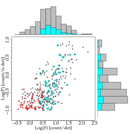
Figure 1 shows the $z$-golden sample together with the full sample of 244 GRBs in the $\log{P}$–$\log{F}$ plane evaluated in the observer frame, where $P$ is the peak rate and $F$ is the count fluence per fully illuminated detector for an on-axis source. While the two samples have similar $P$ distributions, that with known $z$ seems to be biased against low-fluence GRBs. However, a Kolmogorov-Smirnov (K–S) test yields a $9.7$% probability for the two distributions of being drawn from the same population. The $z$-golden sample thus is not inconsistent with being an unbiased selection of the full set in the $\log{P}$–$\log{F}$ plane. From Figure 1 it is also apparent that extrapolating to peak rates below the threshold of $0.1$ count s^-1 det^-1 would not increase the sample of GRBs with useful S/N, because the fraction of rejected GRBs becomes dominant.

2.3 PDS calculation

The choice of the time interval over which the PDS is most conveniently calculated was driven by the need for covering the overall GRB profile as well as optimising the S/N. We verified that the overall shape of the PDS does not depend on the particular choice of the time interval, whereas its S/N clearly does. After a number of attempts, we came up with the following choice: first we found the first ($t_{1}^{(n\sigma)}$) and the last ($t_{2}^{(n\sigma)}$) time bins whose count rates exceeded the background level at $n$$\sigma$ ($n\geq 5$). Let $\Delta_{n\sigma}=t_{2}^{(n\sigma)}-t_{1}^{(n\sigma)}$ be the duration of this interval. The time interval chosen for the PDS calculation starts at $t_{1}^{(n\sigma)}-\Delta_{n\sigma}$ and ends at $t_{2}^{(n\sigma)}+\Delta_{n\sigma}$. If we had chosen a fixed time interval for all GRBs, thus with a common frequency binning scheme, the S/N of the shortest GRBs would have been worse, due to including additional noise with no signal. In the observer frame the bin time was fixed to 64 ms, while for the source rest frame GRBs two rest-frame bin times were used, 4 and 8 ms. We found no noticeable difference between $n=5$ and $n=7$, apart from a different S/N in the average PDS, which led us to finally choose $n=7$. Tables 1–3 report the time intervals for all GRBs in each GRB sample.

In the full sample the duration of this time interval is found to be thrice as long as the GRB duration expressed by its $T_{90}$. Given that the time interval duration is by construction $3\,\Delta_{7\sigma}$, this simply reflects that, on average, $\Delta_{7\sigma}$ does not differ from $T_{90}$ remarkably.

The PDS was obtained through the mixed-radix FFT algorithm implemented within the GNU Scientific Library (Galassi et al., 2009), which does not require the total number of bins to be a power of 2 (Temperton, 1983). Each PDS was calculated adopting the Leahy normalisation, in which the constant power due to statistical noise has a value of 2 (Leahy et al., 1983). Usually the PDS is calculated from the light curves not background-subtracted to ensure that counts are Poisson distributed, and consequently the power distribution is known: e.g., in case of pure statistical noise, the power is $\chi^{2}_{2}$-distributed. In the case of BAT data, the background subtraction through the mask weighting technique is not an issue as explained below.

The average PDS of a given sample of GRBs was obtained assuming two different normalisations: i) the BAT mask-weighted count rates and corresponding errors are normally distributed and there is no evidence for any extra variance (down to a few percent) in addition to the statistical white noise (Rizzuto et al., 2007). The uncertainties on the power of the individual PDSs were calculated according to Guidorzi (2011). From Parseval’s theorem the integral of each individual noise-subtracted PDS yields the net variance, i.e. removed of the statistical noise. In this case each PDS was normalised by its net variance. This normalisation is preferable, because all GRBs have equal weights in the average PDS. ii) Each GRB light curve is normalised by its peak rate, which allows us to make a direct comparison with BSS98 and BSS00. Hereafter, the two cases are referred to as the (net) variance and the peak normalisations, respectively. A possible third normalisation based on the count fluence was soon neglected, due to the results on the binned average PDSs, which were statistically poorer and less constraining than for the other normalisations. Using different normalisations allows us to evaluate the effects of this kind of choice.

The statistical noise was removed differently in the two cases: in i) the noise was assumed to be perfectly Poissonian (Rizzuto et al., 2007), and calculated consequently. In ii) it was obtained from fitting the average PDS with a constant at sufficiently high frequencies.

We started from a uniform frequency binning scheme with a step of $0.01$ Hz. At $f<0.01$ Hz we considered two bins, $0.001$ Hz $\leq f<0.005$ Hz and $0.005$ Hz $\leq f<0.01$ Hz. For each frequency bin and for each individual GRB we calculated the average power. Finally, for each frequency bin we averaged out the power over all the GRBs of a given sample. The average power in each bin is approximately normally distributed with $\sigma=\sigma_{\rm p}/\sqrt{n}$, where $\sigma_{\rm p}$ is the standard deviation of the corresponding power distribution and $n$ the size of the array, i.e. roughly the size of a given GRB sample. Its validity is ensured by the central limit theorem. $\sigma$ was therefore taken as the uncertainty of the corresponding average power. Finally the frequency bins of the average noise-subtracted PDS were grouped by requiring at least 3$\sigma$ significance.

2.4 PDS modelling

We modelled the average PDSs with a smoothly broken power-law as in equation (1),

$${\rm PDS}(f)=2^{1/n}\,F_{0}\ \Big{[}\Big{(}\frac{f}{f_{\rm b}}\Big{)}^{n\,\alpha_{1}}+\Big{(}\frac{f}{f_{\rm b}}\Big{)}^{n\,\alpha_{2}}\Big{]}^{-1/n}\qquad,$$ (1)

where the following parameters were left free to vary: the break frequency $f_{\rm b}$, the value of the PDS at the break frequency $F_{0}$, the two power-law indices $\alpha_{1}$ and $\alpha_{2}$ ($\alpha_{2}>\alpha_{1}$). Initially, the peakedness parameter $n$ was also left free to vary. However in most cases the data were not sensitive to it, so we fixed $n=10$ for all cases to ensure a more homogeneous comparison between the best-fit values obtained over different sets. This choice implies a rather sharp break around $f_{\rm b}$.

In Section 3.6 we discuss more in detail how much the results, especially $\alpha_{2}$, depend on this degree of freedom. The best-fit model is obtained by minimising the total $\chi^{2}$.

3 Results

Table 4 reports the best-fit parameters of the model in equation (1) for each GRB sample and both normalisations. Parameters’ uncertainties are given at 90% confidence level for one parameter of interest.

Figure 2: Average PDS for the full sample of 244 GRBs in the observer frame. Crosses (empty circles) correspond to the net variance (peak rate) normalisation case. Upper limits are 2$\sigma$. The peak rate data have conveniently been shifted for the sake of clarity. The corresponding best fit broken power-laws are also shown. Notably, the peak normalisation has a poorer S/N due to the bright GRBs having a smaller weight than in the variance normalisation; this becomes apparent at high frequencies, where the signal becomes comparable with statistical noise.

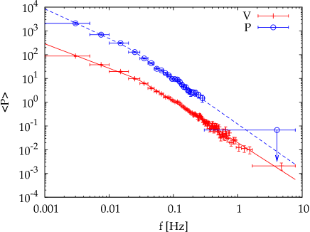
Figure 2 displays the average PDS of the full sample for both normalisations as well as their corresponding best-fit models. The variance-normalised PDS has a best-fit value around $1.03\pm 0.05$ for $\alpha_{1}$, followed by a break around $3\times 10^{-2}$ Hz, above which the slope becomes $\alpha_{2}=1.73_{-0.03}^{+0.04}$. The peak-normalised PDS has a similar value for $f_{\rm b}$, and steeper values for the the power-law indices: $\alpha_{1}=1.25_{-0.12}^{+0.11}$ and $\alpha_{2}=1.90_{-0.06}^{+0.07}$. The difference $(\alpha^{\rm(peak)}_{i}-\alpha^{\rm(var)}_{i})$ in the power-law indices between the two normalisations is found to be in the range $0.1$–$0.2$ for all the GRB subsamples considered, although it is always compatible with zero at $3$$\sigma$.

Figure 3: Average source rest frame PDS for the $z$-silver sample of 97 GRBs in the observed 15–150 keV energy band. Symbols are the same as in Fig. 2.

Figure 4: Top Panel: average source rest frame PDS for the $z$-golden sample in the common 66–366 keV source rest frame energy band. Bottom Panel: average PDS for the same sample in the 15–150 keV energy band (observer frame). Symbols are the same as in Fig. 2.

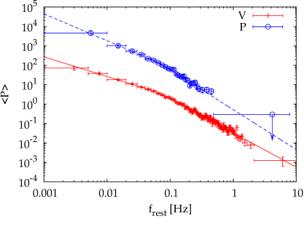
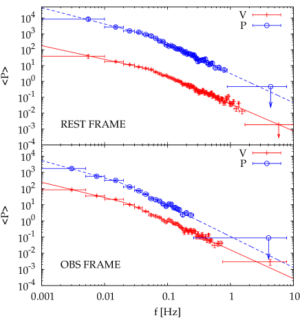
The value of $\alpha_{2}$ is very similar to the power-law index $1.67\pm 0.02$ in the range $0.02<f<1$ Hz in the 50–300 keV band found by BSS98, and between $1.50$ and $1.72$ in the range $0.025<f<1$ Hz in the 20–2000 keV band found by BSS00. Very similar results are obtained for the $z$-silver and golden samples (Figs. 3 and 4), apart from the best-fit values of $f_{\rm b}$ which are higher in the source rest frame. This is no wonder, and links to the cosmological time dilation. This is quantified by fitting the average PDS of the $z$-golden sample in the observer frame: moving from observer to source rest frame, $f_{\rm b}$ changes from $2.4\times 10^{-2}$ to $5.3\times 10^{-2}$ Hz. The ratio of $2.2\pm 0.6$ between the source- and the observer-frame values of $f_{\rm b}$ is close to the average factor of $(1+\hat{z})\sim 3.2$, where $\hat{z}=2.2$ is both median and mean redshift of the $z$-golden sample. Except for $f_{\rm b}$, the comparison of the results obtained for the $z$-golden sample between observer and source rest frame shows no significant differences in the power-law indices. The same conclusion holds when we compare the $z$-silver with the full sample. This result is not obvious: although power-law indices are clearly invariant observables, the impact of averaging out different source-frame energy bands on the observed PDS is not obvious.

Figure 5: Top panel: examples of light curves of individual GRBs randomly selected from the full sample. Data are shifted along the $y$-axis for clarity. Bottom panel: the corresponding PDSs. Dashed lines are power-laws with index $5/3$.

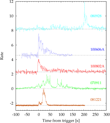
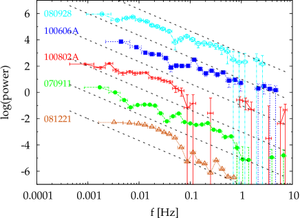
Figure 5 shows examples of light curves and their PDSs of individual GRBs randomly picked out from the full sample. While the global trend suggested by visual inspection favours the description of the average PDS with a power-law with index compatible with $\sim 1.7$ above a few $10^{-2}$ Hz, individual PDSs still exhibit a variety of different average declines.

3.1 Average PDSs at different energies

Remarkably different behaviours in the high-frequency power-law indices are observed for different observed energy bands: in the variance normalisation, $\alpha_{2}$ varies from $1.75_{-0.04}^{+0.05}$ to $1.49_{-0.07}^{+0.08}$ passing from 15–50 to 50–150 keV. The low-frequency index $\alpha_{1}$ is also shallower at higher energies, $0.91_{-0.14}^{+0.11}$ to be compared with $1.07\pm 0.05$ observed in the softer energy channel (Fig. 6).

Figure 6: Top Panel: average PDS for the full sample in the 15–50 keV energy band (observer frame). Bottom Panel: average PDS for the same sample in the 50–150 keV energy band. Symbols are the same as in Fig. 2.

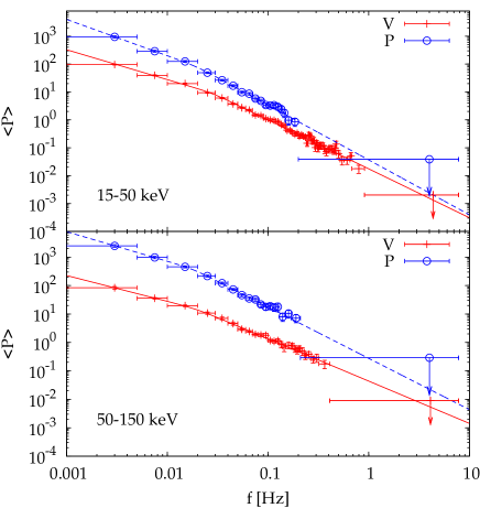
The break frequency shows no significant dependence on energy. Analogous variations are observed in the peak normalisations, although the indices are systematically steeper, as noted above. The same trend was noted in the individual BATSE energy channels: the power-law index decreased from $1.72$ in the 25–55 keV to $1.50$ above 320 keV (BSS00).

Figure 7: High-frequency power-law index $\alpha_{2}$ as a function of energy $E$ obtained by fitting the average PDS of the full sample within the variance (crosses) and the peak (circles) normalisations. BSS00 results derived from BATSE GRBs are also shown (squares). The dashed line shows the power-law $\alpha_{2}\propto E^{-0.05}$.

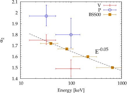
Figure 7 directly compares our values with BSS00’s as a function of energy. The BATSE data show a dependence on energy $E$ which can be modelled with the power-law $\alpha_{2}\propto E^{-0.05}$. These results are compatible with ours within uncertainties (BSS00 do not provide uncertainties on their values). Curiously, the variance normalisation, which is preferable to us also for the reasons explained below in Section 3.7, is in better agreement with BSS00 results than the peak normalisation, which BSS00 adopted for their analysis.

3.2 The effects of GRB durations

The cut-off frequency $f_{\rm b}$ is mainly connected with the average duration of the GRBs and of the individual pulses they consist of, as noted above when moving from the observer to the source rest frame. We investigated the role of the duration by selecting two subsets of the full sample with extreme durations, each collecting 90 GRBs.

In principle, because of the finiteness of the GRB duration, and therefore of the temporal window which contains its time profile, the observed PDS is the convolution of the true one with $|\sin{(f\,\pi\,T)}/(f\,\pi)|^{2}$, where $f$ is frequency and $T$ is the length of the window (e.g., van der Klis 1989). In practice, all the features in the true PDS narrower than $1/T$ are smoothed out, and the minimum frequency that can be explored, $1/T$, also defines the resolution of the PDS. Provided that $T\gg\tau$, where $\tau$ is a generic characteristic time scale acting in a GRB, the cut-off frequency associated to it, $\approx 1/\tau$, is unaffected.

Figure 8 shows the duration distributions for the full sample as well as for the two subsets chosen by us: GRBs with $T_{90}<40$ s, $T_{90}>80$ s on the other side. The top panel of Figure 9 displays the average PDS of both subsamples.

Figure 8: $T_{90}$ distribution for the full sample (solid line). Shaded histograms show two subsets including 90 GRBs each with the shortest and longest durations, respectively.

Figure 9: Top Panel: average PDS for two subsets with extreme durations: 90 shortest vs. 90 longest duration GRBs. Bottom Panel: average PDS for two subsets with extreme count fluences: 30 highest-fluence vs. 97 lowest-fluence GRBs. The thick solid lines is the best fit for the full sample. Different data sets are shifted for clarity reasons.

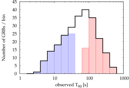
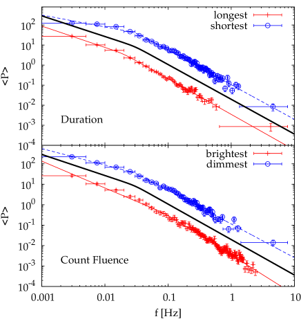
The logarithmic average durations of each subsample are $15$ and $153$ s, respectively. Indeed, $f_{\rm b}$ decreases from $3.2\times 10^{-2}$ of the shortest GRBs to $2.0\times 10^{-2}$ Hz of the longest ones (Table 4). The change of $f_{\rm b}$ is not comparable to the corresponding change in the average duration. However, the low-frequency power-law index $\alpha_{1}$ significantly steepens from $\sim 0.6$ to $\sim 1.1$ in the variance normalisation. This suggests that different values of $f_{\rm b}$ may affect the estimate of $\alpha_{1}$, because the asymptotic behaviour is not reached when $f_{\rm b}$ is close to the lowest explorable frequency, and is more affected by the finite width at low frequencies. Moreover, the cut-off frequency is more sensitive to the average characteristic times (both rise and decay times) of individual shots, rather than to the overall duration: e.g., the PDS of a simple exponential shot with a characteristic time $\tau$ has $f_{\rm b}\sim 1/2\pi\tau$ (e.g., Lazzati 2002). This is still true in the presence of shot noise (Frontera & Fuligni, 1979; Belli, 1992), provided that the occurrence times of the shots are independently distributed. Although this is a rough approximation in this case, the best-fit values of $f_{\rm b}$ imply characteristic times of individual shots about 5–8 s (2–4 s) long in the observer (source rest) frame.

3.3 The effects of GRB peak rates and fluences

Similarly, we investigated the effects of both the peak count rate and fluence on the average PDS by selecting proper subsets of the full sample. Unlike for the duration, the S/N does depend on both peak rate and fluence. We ensured comparable statistical quality of the two subsets by collecting more faint bursts (both in terms of peak rates and count fluence). As for the peak rate $p$, we ended up with 124 and 65 GRBs with $p<0.4$ count s^-1 det^-1, and $p>1.0$ count s^-1 det^-1, respectively. The fluence $F$-selected subsets include 97 and 30 bursts with $F<4.4$ count det^-1, and $F>19.8$ count det^-1, respectively. Both peak rate and count fluence distributions are shown in the projected histograms of Fig. 1.

Concerning the peak rate, the best-fit power-law indices are the same for both subsamples. Instead, $f_{\rm b}$ increases by a factor of 3 (5) in the variance (peak) normalisation when we move from the faint to the bright subset. This is due to the brighter pulses being narrower (Norris et al., 1996): on average the GRBs of our faint subset have 3 to 5 times longer pulses than those of the bright subset. This seems to be at variance with the results by BSS00, who found a decreasing power-law index with increasing peak count rate: from $1.82$ for the faintest GRBs down to $1.63$ for the brightest end.

Concerning $\alpha_{1}$, only for the count fluence sample this index becomes shallower when moving from the high- to low-fluence subset. The same behaviour is observed for the duration-driven subsamples (Section 3.2) when we move from the longest to the shortest GRBs. This common property is explained by the shortest GRBs having lower fluence on average, as confirmed by the correlation between fluence and $T_{90}$ for both the full and the $z$-silver samples with significance values of the order of $10^{-11}$ and $0.1$–$0.2$%, respectively, according to the non-parametric tests of Spearman and Kendall.

We note that the estimate of the power-law index within a given range can be affected by the choice of the model: from fig. 8 of BSS00, the range over which the power-law is fitted extends over a single decade. Within such a limited range the fitted slope is sensitive to the frequency interval chosen for modelling. Within our data, when we opt for a smoother break in equation (1) by fixing $n=1$, the best-fit values for the post-break frequency slope $\alpha_{2}$ are systematically steeper, because the asymptotic value is not reached within the range covered by the data (Section 3.6).

In equation (1) this may introduce an artificial correlation between $f_{\rm b}$ and $\alpha_{2}$ (as well as $\alpha_{1}$): the higher $f_{\rm b}$, the steeper $\alpha_{2}$, when the frequency range covered by the data is not sufficiently broad. Indeed, we observe this in the fluence-driven subsets, as reported in Table 4 and shown in the bottom panel of Fig. 9. Only in the variance normalisation case, $\alpha_{2}$ varies from $1.65$ (faint subset) to $1.94$ (bright subset), whereas $f_{\rm b}$ increases by a factor of $3.1$. No such change is observed in the peak normalisation case, where both $f_{\rm b}$ and $\alpha_{2}$ experience very little changes.

We checked whether the results obtained on the fluence-driven subsets are affected by the corresponding average S/N. We split the sample in two subsets of 50 and 150 GRBs having the highest- and lowest-S/N PDSs, respectively. Within uncertainties the two average PDSs showed no distinctive behaviour. Therefore, the variety of S/N is not directly responsible for the different PDS properties of fluence-driven subsets.

3.4 The effects of different $E_{\rm iso}$ and $L_{\rm p,iso}$

Here we investigate the possible existence of correlations between the PDS and intrinsic properties of the prompt emission. Out of the $z$-silver sample, we selected the GRBs with measured intrinsic peak energy of the time-averaged $E\,F(E)$ spectrum, the so-called $E_{\rm p,i}$. The isotropic-equivalent gamma-ray released energy in the $1$–$10^{4}$ keV band, $E_{\rm iso}$, which correlates with $E_{\rm p,i}$ (Amati et al., 2002), is also known for the same events. We adopted the standard cosmological model: $H_{0}=71$ km s^-1 Mpc^-1, $\Omega_{\Lambda}=0.73$, $\Omega_{M}=0.27$ (Spergel et al., 2003). The values for both $E_{\rm p,i}$ and $E_{\rm iso}$ are taken from Amati et al. (2008; 2009; in prep.). We ended up with a subset of 64 GRBs. For the same bursts we estimated the isotropic-equivalent peak luminosity, $L_{\rm p,iso}$, by normalising $E_{\rm iso}$ through the ratio between peak count rate and count fluence in the source-rest frame. This implicitly assumes no spectral evolution throughout the prompt emission, which for instance does not hold when the hardness ratio tracks the time profile. This leads to underestimating the peak luminosity by a factor of a few in the worst case. However, in a logarithmic space this cannot wash out possible genuine correlations or build fake ones, but it may merely increase the observed dispersion. The values of $E_{\rm iso}$, $E_{\rm p,i}$, and $L_{\rm p,iso}$ for this subsample are reported in Table 5.

We compared the average PDS of the least and that of the most energetic GRBs as follows: we collected two subsets of 25 GRBs each, with extreme values of $E_{\rm iso}$. Each subset collects about 1/3 of the overall set. The least energetic GRBs all have $E_{\rm iso}<9\times 10^{52}$ ergs, while the most energetic ones all have $E_{\rm iso}>2.1\times 10^{53}$ ergs, with logarithmic average values of $2.8\times 10^{52}$ and $4.7\times 10^{53}$ ergs, respectively. The average PDS of the two groups are not found to significantly differ from one another, as reported in Table 4.

Analogously, we divided the same sample according to different classes of $L_{\rm p,iso}$ and in none of the cases we found evidence for a dependence of the average PDS on $L_{\rm p,iso}$.

3.5 The effects of redshift

We considered two classes of 32 GRBs each with the lowest and highest redshift values, respectively, among the $z$-silver sample. The aim is to study possible evolutionary effects. The choice of the number of GRBs is a trade-off between the need for a big enough sample for statistical purposes, and the need of having two well separated redshift bins. We came up with two classes: the low-$z$ GRBs with $0.1<z<1.5$, and the high-$z$ ones with $2.6<z<8.1$. The mean (median) redshifts for both subsets are $0.9$ ($0.9$) and $3.5$ ($3.2$), respectively. The corresponding average PDSs are shown in Figure 10 together with their best-fit models (Table 4).

Figure 10: Average source-rest frame PDS for two subsets with different redshift bins taken from the $z$-silver sample: low-$z$ (filled squares), and high-$z$ (empty circles), together with their corresponding best-fit models. For comparison, the thick solid line shows the best-fit model obtained over the entire $z$-silver sample.

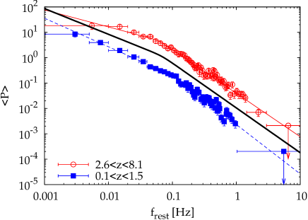
Similarly to what is observed for the low-fluence GRBs, for the variance normalisation the average PDS of high-$z$ GRBs has shallower indices: $\alpha_{1}$ and $\alpha_{2}$ are respectively $0.67_{-0.22}^{+0.17}$ and $1.71_{-0.07}^{+0.08}$, to be compared with $1.12\pm 0.08$ and $1.95_{-0.11}^{+0.12}$ found for the low-$z$ GRBs. To understand whether this is due to the farther GRBs having lower fluence values on average, in Figure 11 we studied the correlation between fluence and redshift for the full $z$-silver sample as well as for the two subsets here considered.

Figure 11: Count fluence vs. redshift $z$ distribution for the $z$-silver sample. The two subsets with different redshift bins are also shown with the same symbols as in Fig. 10.

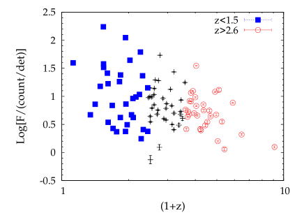
There is a hint for an anticorrelation between observed fluence and redshift, whose significance is about $0.2$–$0.3$% according to non-parametric tests (Spearman, Kendall). The fluence distributions of the low- and of the high-$z$ subsets have a K–S probability of $1.6$% of being drawn from the same population. As for the fluence, the $z$-silver sample is an unbiased subset of the full sample, since the two fluence distributions are fully compatible (46% probability according to a K–S test). Thus, the low-fluence subset of the full sample discussed in Section 3.3 is likely to include more high-$z$ bursts than what the high-fluence subset does. On average, the high-fluence bursts have lower redshifts and this explains the common properties observed in the average PDS, compared with that of low-fluence and high-redshift GRBs. Given the correlation between fluence and $T_{90}$, we checked whether for the $z$-silver sample the redshift also correlates with the observed $T_{90}$, and we found it does not. Therefore, while the fluence correlates with $T_{90}$ and anticorrelates with redshift, the latter does not correlate with $T_{90}$.

Qualitatively, the shallower power-law indices for the low-fluence/high-$z$ GRBs can be explained by the result found on the average PDSs of different energy channels (Section 3.1 and Fig. 7): harder photons have a shallower PDS (see also Table 4). Given that the light curves of the $z$-silver sample refer to the common observed 15–150 keV energy band, the results obtained for the high-$z$ subset refer to a harder source-rest frame energy band. Whether this difference between the average PDS of low- and that of high-$z$ GRBs can entirely be ascribed to the cosmological shift of the energy band, or it is due to an evolutionary property of GRBs is not clear. To clarify this issue, we should apply the same analysis to the $z$-golden sample: however, practically this is not feasible due to the low number of GRBs, the limited range both in $z$ (Section 2.2) and in fluence (Fig. 1).

3.6 Smoothness of the break

In Section 3.3 we noted that choosing a smoother break in equation (1), e.g. $n=1$ instead of $n=10$, yields systematically shallower (steeper) values for $\alpha_{1}$ ($\alpha_{2}$). The differences in $\alpha_{2}$ between $n=10$ and $n=1$ are however milder and in all cases they are compatible with zero within uncertainties. Analogously, $f_{\rm b}$ is systematically lower for a smoother break, although not significantly. Overall, allowing the data to be fitted with a smoother break implies that the asymptotic regime at low frequencies is not covered by the data, and this leads to shallower values for $\alpha_{1}$ than what data actually exhibit. The goodness of the fits in both cases is similar and shows no systematic behaviour.

We conclude that the degree of freedom brought in by the smoothness of the break of equation (1) does not affect significantly the estimates of $\alpha_{2}$, thanks to the broader frequency range at $f>f_{\rm b}$ covered by the data.

3.7 PDS distribution

PDSs of individual GRBs are very different from each other (Fig. 5). For instance, let us consider a single fast-rise exponential decay (FRED) with a characteristic time $\tau$ (either rise or decay time). At $f\gg 1/\tau$ the PDS asymptotically declines as a power-law with an index of 2 or steeper. Depending on the peakedness value, the PDS can also exhibit oscillatory terms in the decay, as shown by Lazzati (2002). Oscillations modulating the power-law decline can also appear in the PDS of those GRBs with two or more pulses separated by a quiescent time, which makes them interfere in the Fourier transform (since the PDS can also be seen as the Fourier transform of the autocorrelation function, as stated by the Wiener-Khinchin theorem).

When for each frequency bin we average out the power for a given set of GRBs, we implicitly assume that each time profile is an individual realisation of a common stochastic process. On the contrary, if one is interested in studying the light curve of a single GRB, and treats it like a deterministic signal affected by uncorrelated noise, the averaging process does not make sense any more (e.g., Guidorzi, 2011).

Under the assumption of a unique stochastic process explaining the variety of observed GRB light curves, we study the power distribution as a function of frequency. BSS98 found that for peak normalisation for a given frequency bin $f_{j}$, the fluctuations $P_{i}(f_{j})$ around the average power $\bar{P}(f_{j})$ ($i$ running over a given set of GRBs) are minimal, and the distribution is an exponential, $dN/dP(f_{j})=N\,\exp{[-P(f_{j})/\bar{P}(f_{j})]}$. For each grouped frequency bin we investigated the observed distribution. For both normalisations we did not subtract the Poisson noise.

Figure 12: Observed distributions of the power at four different frequency bins from the full sample: from top to bottom, left to right, $0.01$–$0.02$, $0.05$–$0.06$, $0.23$–$0.24$, and $0.40$–$0.41$ Hz, respectively. Dashed lines show the corresponding expected exponential distribution, $dN/dP\propto\exp{(-P/\bar{P})}$.

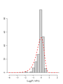
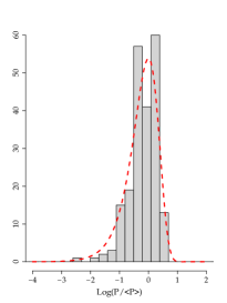
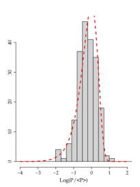
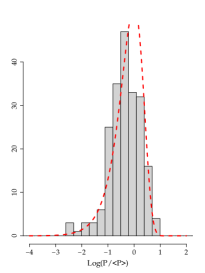
Figure 12 displays four distributions corresponding to four different frequency bins for the full sample of GRBs in the variance normalisation. We adopted the Anderson–Darling test (Anderson & Darling, 1952) implemented under the $R$ package ADGofTest (v0.1) to test the compatibility with an exponential. This test is particularly sensitive to the distribution tails and, as such, to the possible presence of a few outliers. The corresponding probability was evaluated as a function of frequency for both normalisations and for different GRB sets. The results are shown in the top panels of Figure 13. We also studied the ratio between the standard deviation of the observed distribution and that expected in the exponential distribution hypothesis (bottom panels of Fig. 13).

Figure 13: Top panel: P-value based on the Anderson-Darling test that the corresponding density distribution of power as a function of frequency is consistent with an exponential. The ratio between the $\sigma$ of the observed power distribution over the corresponding average value is also shown. The solid (dashed) line shows the variance (peak) normalisation case. GRBs are from the full sample. Mid panel: the same, with GRBs being taken from the $z$-silver sample. Bottom panel: the same, with GRBs from the $z$-golden sample.

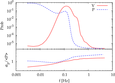
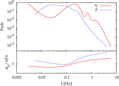
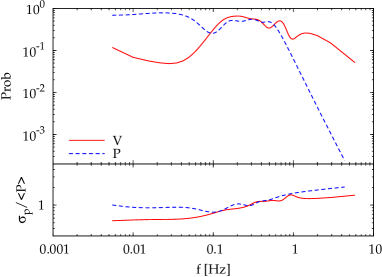
For all the GRB sets the fluctuations of the variance normalisation are systematically lower than in the peak normalisation. In the full sample case (top panel of Fig. 13), at low frequencies the p-value of the variance normalisation is $\approx 10^{-5}$, due to the small dispersion of the distribution compared to that expected for an exponential. At $f\ga$ a few $10^{-2}$ Hz the p-value rises above $0.01$, and finally decreases again below $0.01$ at $f>$ a few $0.1$ Hz. For less numerous sets, such as the $z$-silver and golden samples (mid and bottom panels of Fig. 13, respectively), the exponential hypothesis cannot be rejected at almost any frequency for the variance normalisation. For the peak normalisation, the high-frequency range ($f\ga 1$ Hz) exhibits systematically worse p-values and larger fluctuations around the average power.

In conclusion, the variance normalisation shows minimal fluctuations around the average power and the PDS is distributed most consistently with an exponential. This is also a $\chi^{2}$ distribution with two degrees of freedom ($\chi^{2}_{2}$), and suggests that the properly normalised power of each GRB at any given frequency is the result of a Fourier transform term, whose amplitude is normally distributed around the average value and the phase is independently and uniformly distributed (van der Klis, 1989). The fluctuations around the mean value become significantly larger than what expected for a $\chi^{2}_{2}$ distribution above $\sim$1 Hz in the largest samples (Fig. 13). In our data at these frequencies the statistical noise becomes comparable with signal, and this could be connected with it, although the details are not clear. Alternatively, it could be suggestive of the presence of a fraction of GRBs with significantly more power at high frequencies than the bulk of GRBs.

Concerning the relative weight of some GRBs in driving the average results, none of the classes considered above (Sections 3.2, 3.3, and 3.4) seems to be dominant in determining the observed properties, especially the high-frequency slope $\alpha_{2}$. By definition, the variance normalisation equally weighs each GRB in the average (noise–subtracted) PDS, since the normalised PDSs of both bright and dim GRBs have the same area. The only difference is that dim GRBs have a lower S/N, and, as a consequence, they can contribute more than bright GRBs to the observed scatter in the power distribution.

4 Conclusions

For the first time it was possible to study the average PDS of a sample of long GRBs by correcting for the cosmological time dilation effects both on timing and spectral properties. This is described by a smoothed broken power-law, with a typical low- (high-) frequency index around $1.0$ ($1.7$–$1.8$), and a break frequency of a few $\times 10^{-2}$ Hz. This is mainly determined by an average rest–frame characteristic time of 2–4 s for the individual shot most GRBs are made of. We found no clear difference from what is obtained by processing the same sample within the observer frame, apart from the break frequency $f_{\rm b}$. In particular, for a restricted sample of 64 GRBs with known $E_{\rm iso}$, $L_{\rm p,iso}$ we found no correlation between intrinsic properties and the average rest–frame PDS.

Comparing different energy bands, in agreement with previous results we found that the average PDS in the harder energy channel exhibits shallower indices, especially at high frequencies. From the sample of GRBs with known redshift, we found that in the observed 15–150 keV energy band the average PDS of the high-$z$ GRBs, which also have lower fluences on average, exhibits marginally shallower indices than the average PDS of the low-$z$/higher-fluence GRBs. In principle, this can be explained by the farthest GRBs being observed in source-rest frame harder energy bands. Whether this property is entirely due to the cosmological energy band shift bias, or it implies some evolution in the average PDS with redshift, cannot be settled with the present dataset, because of the narrow passband of BAT.

In the observer frame the shortest GRBs ($3$ s $<T_{90}<40$ s), which on average have lower fluences as well, are characterised by higher values of $f_{\rm b}$ and shallower values of the low-frequency power-law index. This suggests that, within the covered frequency range, they better approach the asymptotic value of a flat PDS at low frequencies.

In most cases the high-frequency index for different GRB samples is compatible with $5/3$ expected for a Kolmogorov velocity spectrum in a turbulent medium, but in fewer cases can also be as steep as $\sim 2$ with no break in the power-law up to several Hz.

At variance with past results, we do not find evidence for any cut-off around 1–2 Hz in the average PDS. Instead, for the full and the $z$-silver samples the average PDS is consistent with an unbroken power-law up to several Hz at the least (Figs. 2 and 3). However, the softer energy band of BAT compared with that of BATSE might account for the missing cut-off above 1 Hz.

Theoretical interpretations of the power-law PDS with an index compatible with $5/3$ have been proposed in several different contexts. Within the internal shock model, by tuning the flow of mass and energy emission through the wind of shells it is possible to obtain the average power-law in the PDS (Panaitescu et al., 1999; Spada et al., 2000). The observed PDS index is also obtained from emission due to a relativistic outflow of a jet propagating through the stellar and the circumstellar matter (Zhang et al., 2009; Morsony et al., 2010).

Alternatively to the classical internal shock model in which the energy of the ejecta is mostly kinetic, in the magnetically-dominated outflows the energy dissipation via magnetic reconnection plays a crucial role (e.g., Lyutikov 2006; Zhang & Yan 2011; and references therein). In the ICMART model, the rapid reconfiguration of the magnetic field can trigger MHD turbulence, which ends up in a runaway release of synchrotron gamma-rays radiated by the accelerated particles. Unlike the hydrodynamical turbulence characterised by the $5/3$ Kolmogorov velocity spectrum, MHD turbulence scales differently for different directions with respect to the field lines: the index ranges from $5/3$ to $2$ moving from perpendicular to parallel direction (Zhang & Yan, 2011). Interestingly, this range matches our results.

Within some models, the observed variability may track that of the progenitor, e.g. through erratic accretion episodes (e.g., Kumar et al. 2008), or hydrodynamical or magnetic instabilities in the accretion disc (e.g., Perna et al. 2006; Proga & Zhang 2006; Margutti et al. 2011). In particular, variability can also arise from turbulence within the accretion disc. For instance, in the context of magneto-rotational instability, Carballido & Lee (2011) studied how neutrino cooling can shape different PDSs of the observed luminosity, depending on the cooling process. Neutrino emissivity scales with temperature $T$ as $\dot{q}\propto T^{\beta}$, where $\beta$ is 9 (6) when $e^{\pm}$ pair annihilation ($e^{\pm}$ capture by free neutrons or protons) is the dominant process. They found that the range of power-law indices expected in the average PDS from $0.1$ to $100$ Hz vary between $1.7$ and $2.0$ with no clear break around $1$–$2$ Hz, and with some bumps above $1$–$10$ Hz which flatten the decline. Most of our values for the high-frequency power-law index are closer to $1.7$ (Table 4), and according to the neutrino-cooling interpretation, on average this would favour larger values for $\beta$, i.e. where pair annihilation is dominant. However, due to S/N limitations, our present data set do not allow us to explore the average properties at high ($>10$ Hz) frequencies, and the GRBs with sufficient signal are too few to draw statistically sound conclusions. Hopefully, in the future more numerous samples of GRBs with high S/N especially at high ($>10$ Hz) frequencies will allow us to better discriminate between competing models.

Table 1: Table of the full sample including 244 GRBs in the observer frame.

GRB	$t_{\rm start}$	$t_{\rm stop}$	Log(Count Fluence)	Log(peak rate)	$T_{90}$
	(s)	(s)	(count det-1)	(count s-1 det-1)	(s)
050117	$-203.8$	$302.7$	$1.155\pm 0.007$	$-0.486\pm 0.029$	$200.0$
050124	$-3.7$	$6.6$	$0.265\pm 0.015$	$-0.098\pm 0.033$	$4.1$
050128	$-37.3$	$52.8$	$0.851\pm 0.015$	$0.158\pm 0.042$	$13.8$
050219A	$-30.3$	$47.0$	$0.772\pm 0.011$	$-0.357\pm 0.028$	$23.0$
050219B	$-96.1$	$106.8$	$1.354\pm 0.010$	$0.584\pm 0.028$	$27.0$
050306	$-188.1$	$302.8$	$1.212\pm 0.015$	$-0.362\pm 0.041$	$158.4$
050315	$-179.8$	$191.6$	$0.795\pm 0.015$	$-0.673\pm 0.037$	$40.0$
050319	$-160.0$	$187.0$	$0.406\pm 0.030$	$-0.767\pm 0.043$	$10.0$
050326	$-49.2$	$68.9$	$1.120\pm 0.005$	$0.284\pm 0.018$	$29.5$
050401	$-43.5$	$64.8$	$1.105\pm 0.014$	$0.176\pm 0.030$	$33.0$
050418	$-92.8$	$163.9$	$0.936\pm 0.012$	$-0.339\pm 0.022$	$83.0$
050502B	$-34.6$	$20.7$	$-0.085\pm 0.031$	$-0.616\pm 0.034$	$17.5$
050505	$-63.8$	$97.3$	$0.550\pm 0.028$	$-0.684\pm 0.042$	$60.0$
050525A	$-12.3$	$25.1$	$1.416\pm 0.002$	$0.829\pm 0.007$	$5.2$
050603	$-26.4$	$41.7$	$1.078\pm 0.013$	$0.846\pm 0.027$	$12.0$
050607	$-19.0$	$37.3$	$0.057\pm 0.027$	$-0.902\pm 0.041$	$26.5$
050701	$-10.1$	$33.0$	$0.411\pm 0.011$	$-0.420\pm 0.026$	$40.0$
050713A	$-112.6$	$223.9$	$0.911\pm 0.012$	$-0.211\pm 0.024$	$70.0$
050713B	$-109.7$	$230.4$	$0.875\pm 0.032$	$-0.717\pm 0.050$	$75.0$
050715	$-150.0$	$224.0$	$0.529\pm 0.024$	$-0.843\pm 0.039$	$52.0$
050716	$-93.8$	$147.1$	$0.979\pm 0.013$	$-0.608\pm 0.030$	$69.0$
050717	$-89.0$	$178.1$	$0.973\pm 0.008$	$0.065\pm 0.038$	$86.0$
050801	$-6.2$	$12.8$	$-0.289\pm 0.034$	$-0.675\pm 0.039$	$20.0$
050803	$-24.2$	$234.5$	$0.573\pm 0.022$	$-0.790\pm 0.045$	$85.0$
050820B	$-14.6$	$29.9$	$0.528\pm 0.008$	$-0.271\pm 0.021$	$13.0$
050822	$-65.0$	$206.8$	$0.732\pm 0.022$	$-0.593\pm 0.037$	$102.0$
050827	$-69.3$	$76.1$	$0.530\pm 0.019$	$-0.617\pm 0.031$	$49.0$
050911	$-17.2$	$32.1$	$-0.273\pm 0.073$	$-0.538\pm 0.055$	$16.0$
050915B	$-50.0$	$98.4$	$0.822\pm 0.010$	$-0.537\pm 0.028$	$40.0$
050922C	$-8.1$	$9.1$	$0.411\pm 0.010$	$0.050\pm 0.025$	$5.0$
051006	$-28.7$	$49.8$	$0.396\pm 0.029$	$-0.346\pm 0.065$	$26.0$
051111	$-60.7$	$103.1$	$0.797\pm 0.011$	$-0.377\pm 0.029$	$47.0$
051113	$-130.2$	$165.1$	$0.664\pm 0.030$	$-0.536\pm 0.046$	$94.0$
051227	$-34.2$	$68.7$	$-0.061\pm 0.044$	$-0.839\pm 0.051$	$8.0$
060105	$-100.0$	$153.4$	$1.393\pm 0.004$	$0.083\pm 0.028$	$55.0$
060110	$-27.4$	$50.4$	$0.462\pm 0.013$	$-0.560\pm 0.024$	$17.0$
060111B	$-61.6$	$117.3$	$0.379\pm 0.034$	$-0.726\pm 0.048$	$59.0$
060115	$-118.1$	$224.4$	$0.546\pm 0.021$	$-0.993\pm 0.034$	$142.0$
060117	$-28.8$	$52.1$	$1.502\pm 0.003$	$0.867\pm 0.017$	$16.0$
060204B	$-166.5$	$264.6$	$0.703\pm 0.017$	$-0.758\pm 0.032$	$134.0$
060206	$-11.4$	$21.8$	$0.211\pm 0.013$	$-0.406\pm 0.018$	$7.0$
060210	$-299.8$	$302.3$	$1.093\pm 0.015$	$-0.349\pm 0.041$	$46.0$
060223A	$-14.1$	$22.2$	$0.058\pm 0.027$	$-0.782\pm 0.039$	$11.0$
060223B	$-17.7$	$16.6$	$0.417\pm 0.012$	$-0.280\pm 0.038$	$10.2$
060306	$-63.8$	$124.1$	$0.560\pm 0.020$	$0.022\pm 0.028$	$61.0$
060312	$-100.5$	$118.2$	$0.597\pm 0.015$	$-0.706\pm 0.029$	$43.0$
060322	$-239.2$	$477.8$	$0.915\pm 0.017$	$-0.606\pm 0.025$	$213.0$
060403	$-37.0$	$55.5$	$0.306\pm 0.020$	$-0.904\pm 0.031$	$30.0$
060413	$-60.0$	$320.0$	$0.846\pm 0.011$	$-0.900\pm 0.024$	$150.0$
060418	$-171.4$	$285.8$	$1.160\pm 0.009$	$0.073\pm 0.038$	$52.0$
060421	$-16.4$	$24.5$	$0.287\pm 0.015$	$-0.397\pm 0.027$	$11.0$
060424	$-58.0$	$59.4$	$0.109\pm 0.042$	$-0.521\pm 0.049$	$37.0$
060428A	$-54.8$	$89.9$	$0.456\pm 0.017$	$-0.571\pm 0.026$	$39.4$
060502A	$-29.1$	$41.5$	$0.555\pm 0.013$	$-0.685\pm 0.021$	$33.0$
060507	$-202.8$	$380.3$	$0.916\pm 0.017$	$-0.840\pm 0.036$	$185.0$
060510A	$-23.3$	$29.5$	$1.229\pm 0.018$	$0.422\pm 0.037$	$21.0$
060526	$-239.2$	$518.0$	$0.432\pm 0.042$	$-0.639\pm 0.043$	$13.8$
060607A	$-126.1$	$214.6$	$0.665\pm 0.015$	$-0.752\pm 0.020$	$100.0$
060607B	$-30.5$	$62.0$	$0.425\pm 0.025$	$-0.807\pm 0.050$	$31.0$
060614	$-166.2$	$327.7$	$1.599\pm 0.004$	$0.441\pm 0.036$	$102.0$
060707	$-114.9$	$86.3$	$0.496\pm 0.027$	$-0.930\pm 0.041$	$68.0$
060708	$-5.8$	$11.8$	$-0.049\pm 0.018$	$-0.573\pm 0.034$	$9.8$
060714	$-134.2$	$233.6$	$0.738\pm 0.021$	$-0.746\pm 0.039$	$115.0$
060719	$-59.9$	$119.6$	$0.431\pm 0.020$	$-0.529\pm 0.034$	$55.0$
060813	$-28.2$	$55.7$	$0.923\pm 0.006$	$0.054\pm 0.012$	$14.9$
060814	$-74.9$	$384.9$	$1.386\pm 0.004$	$-0.031\pm 0.015$	$146.0$
060825	$-10.2$	$14.5$	$0.269\pm 0.012$	$-0.438\pm 0.026$	$8.1$
060904A	$-60.0$	$208.1$	$1.133\pm 0.005$	$-0.130\pm 0.023$	$80.0$
060904B	$-173.7$	$347.0$	$0.453\pm 0.036$	$-0.467\pm 0.031$	$192.0$
060908	$-29.3$	$32.2$	$0.606\pm 0.012$	$-0.305\pm 0.033$	$19.3$
060912A	$-5.5$	$10.3$	$0.381\pm 0.013$	$0.049\pm 0.021$	$5.0$
060927	$-24.7$	$47.0$	$0.325\pm 0.017$	$-0.404\pm 0.023$	$22.6$
061004	$-5.1$	$12.5$	$0.032\pm 0.016$	$-0.399\pm 0.027$	$6.2$
061007	$-39.9$	$357.9$	$1.802\pm 0.002$	$0.431\pm 0.023$	$75.0$
061019	$-239.5$	$64.0$	$0.683\pm 0.058$	$-0.700\pm 0.056$	$191.0$
061021	$-54.5$	$109.2$	$0.673\pm 0.012$	$-0.059\pm 0.018$	$46.0$
061121	$-135.1$	$268.2$	$1.372\pm 0.003$	$0.546\pm 0.014$	$81.0$
061126	$-86.2$	$156.8$	$0.998\pm 0.009$	$0.147\pm 0.017$	$191.0$
061202	$9.8$	$196.2$	$0.574\pm 0.014$	$-0.656\pm 0.028$	$91.0$
061222A	$-113.5$	$219.6$	$1.131\pm 0.006$	$0.270\pm 0.019$	$72.0$
070103	$-18.2$	$37.1$	$-0.191\pm 0.047$	$-0.676\pm 0.064$	$19.0$
070107	$-24.0$	$662.2$	$0.902\pm 0.015$	$-0.637\pm 0.026$	$333.8$
070220	$-187.1$	$345.9$	$1.216\pm 0.007$	$-0.098\pm 0.020$	$129.0$
070306	$-239.2$	$487.7$	$0.991\pm 0.015$	$-0.295\pm 0.019$	$210.0$
070318	$-63.9$	$125.6$	$0.628\pm 0.013$	$-0.624\pm 0.024$	$63.0$
070328	$-90.0$	$227.2$	$1.126\pm 0.006$	$-0.256\pm 0.020$	$69.0$
070411	$-124.1$	$197.7$	$0.704\pm 0.016$	$-0.948\pm 0.035$	$101.0$
070419B	$-239.9$	$400.0$	$1.118\pm 0.008$	$-0.765\pm 0.023$	$236.5$
070420	$-187.4$	$230.4$	$1.360\pm 0.010$	$-0.093\pm 0.026$	$77.0$
070427	$-11.0$	$23.8$	$0.159\pm 0.015$	$-0.716\pm 0.038$	$11.0$
070508	$-46.6$	$73.1$	$1.464\pm 0.002$	$0.572\pm 0.015$	$20.9$
070521	$-70.3$	$97.7$	$1.096\pm 0.006$	$0.060\pm 0.022$	$37.9$
070529	$-115.9$	$237.8$	$0.638\pm 0.033$	$-0.659\pm 0.071$	$109.0$
070612A	$-239.0$	$514.2$	$1.227\pm 0.018$	$-0.805\pm 0.030$	$370.0$
070616	$-89.9$	$963.1$	$1.528\pm 0.004$	$-0.563\pm 0.029$	$402.0$
070621	$-45.5$	$77.0$	$0.845\pm 0.011$	$-0.449\pm 0.038$	$33.3$
070628	$-76.2$	$59.0$	$0.765\pm 0.016$	$-0.264\pm 0.017$	$39.1$
070704	$-239.0$	$732.8$	$0.999\pm 0.013$	$-0.592\pm 0.017$	$380.0$
070721B	$-239.4$	$542.7$	$0.757\pm 0.025$	$-0.720\pm 0.036$	$340.0$
070808	$-28.9$	$55.2$	$0.265\pm 0.027$	$-0.573\pm 0.036$	$32.0$
070911	$-283.5$	$302.8$	$1.347\pm 0.005$	$-0.210\pm 0.026$	$162.0$
070917	$-11.4$	$22.6$	$0.489\pm 0.009$	$0.054\pm 0.016$	$7.3$
071001	$-54.6$	$110.7$	$0.208\pm 0.031$	$-0.985\pm 0.046$	$58.5$
071003	$-182.6$	$342.7$	$1.036\pm 0.014$	$-0.139\pm 0.024$	$150.0$
071010B	$-75.6$	$77.1$	$0.861\pm 0.007$	$-0.111\pm 0.012$	$35.7$
071011	$-64.7$	$119.3$	$0.495\pm 0.029$	$-0.714\pm 0.056$	$61.0$
071020	$-12.8$	$16.9$	$0.507\pm 0.007$	$0.119\pm 0.018$	$4.2$
071025	$-131.5$	$383.7$	$1.067\pm 0.009$	$-0.773\pm 0.028$	$109.0$
071117	$-5.0$	$9.4$	$0.414\pm 0.010$	$0.057\pm 0.023$	$6.6$
080205	$-121.4$	$217.1$	$0.523\pm 0.027$	$-0.899\pm 0.052$	$106.5$
080210	$-35.0$	$39.8$	$0.423\pm 0.018$	$-0.831\pm 0.029$	$45.0$
080229A	$-69.7$	$132.4$	$1.068\pm 0.010$	$0.177\pm 0.039$	$64.0$
080310	$-84.0$	$659.5$	$0.676\pm 0.025$	$-0.953\pm 0.047$	$365.0$
080319B	$-69.6$	$62.2$	$2.057\pm 0.001$	$0.792\pm 0.018$	$125.0$
080319C	$-14.3$	$27.3$	$0.591\pm 0.013$	$-0.186\pm 0.034$	$34.0$
080328	$-115.9$	$225.1$	$1.036\pm 0.010$	$-0.277\pm 0.041$	$90.6$
080409	$-10.0$	$20.4$	$-0.205\pm 0.054$	$-0.481\pm 0.043$	$20.2$
080411	$-78.3$	$155.9$	$1.647\pm 0.002$	$0.743\pm 0.007$	$56.0$
080413A	$-48.2$	$97.4$	$0.734\pm 0.011$	$-0.168\pm 0.015$	$46.0$
080413B	$-6.9$	$11.0$	$0.627\pm 0.011$	$0.280\pm 0.021$	$8.0$
080430	$-20.4$	$40.1$	$0.360\pm 0.015$	$-0.472\pm 0.022$	$16.2$
080503	$-90.8$	$181.6$	$0.487\pm 0.023$	$-0.564\pm 0.063$	$170.0$
080602	$-91.8$	$149.3$	$0.687\pm 0.029$	$-0.326\pm 0.045$	$74.0$
080603B	$-67.5$	$135.4$	$0.639\pm 0.012$	$-0.226\pm 0.028$	$60.0$
080605	$-39.4$	$63.1$	$1.297\pm 0.004$	$0.505\pm 0.023$	$20.0$
080607	$-157.2$	$292.3$	$1.556\pm 0.006$	$0.577\pm 0.028$	$79.0$
080613B	$-86.4$	$157.2$	$0.946\pm 0.007$	$-0.224\pm 0.044$	$105.0$
080623	$-8.7$	$16.0$	$0.181\pm 0.027$	$-0.488\pm 0.059$	$15.2$
080714	$-30.9$	$51.2$	$0.608\pm 0.014$	$-0.252\pm 0.024$	$33.0$
080721	$-34.6$	$39.2$	$1.264\pm 0.013$	$0.513\pm 0.041$	$16.2$
080725	$-50.9$	$55.9$	$0.715\pm 0.013$	$-0.596\pm 0.022$	$120.0$
080727B	$-9.6$	$18.5$	$0.648\pm 0.007$	$0.114\pm 0.022$	$8.6$
080727C	$-113.9$	$222.3$	$0.924\pm 0.010$	$-0.519\pm 0.024$	$79.7$
080804	$-33.5$	$68.6$	$0.713\pm 0.018$	$-0.444\pm 0.033$	$34.0$
080805	$-88.7$	$170.3$	$0.644\pm 0.014$	$-0.846\pm 0.027$	$78.0$
080810	$-122.6$	$220.2$	$0.860\pm 0.012$	$-0.499\pm 0.034$	$106.0$
080903	$-61.9$	$98.0$	$0.489\pm 0.017$	$-0.991\pm 0.055$	$66.0$
080905B	$-96.1$	$191.9$	$0.483\pm 0.032$	$-0.759\pm 0.045$	$128.0$
080906	$-239.4$	$267.3$	$0.830\pm 0.015$	$-0.932\pm 0.022$	$147.0$
080915B	$-4.0$	$6.4$	$0.259\pm 0.012$	$0.025\pm 0.019$	$3.9$
080916A	$-76.4$	$146.2$	$0.839\pm 0.008$	$-0.461\pm 0.016$	$60.0$
080928	$-131.5$	$400.0$	$0.675\pm 0.020$	$-0.495\pm 0.031$	$280.0$
081008	$-239.6$	$338.4$	$0.876\pm 0.013$	$-0.797\pm 0.024$	$185.5$
081102	$-54.7$	$54.2$	$0.551\pm 0.023$	$-0.756\pm 0.037$	$63.0$
081109	$-109.0$	$169.0$	$0.790\pm 0.011$	$-0.791\pm 0.019$	$190.0$
081126	$-85.3$	$106.9$	$0.723\pm 0.012$	$-0.302\pm 0.021$	$54.0$
081128	$-80.0$	$153.5$	$0.681\pm 0.015$	$-0.787\pm 0.037$	$100.0$
081203A	$-141.7$	$255.4$	$1.052\pm 0.008$	$-0.318\pm 0.032$	$294.0$
081210	$-109.9$	$287.1$	$0.546\pm 0.025$	$-0.453\pm 0.028$	$146.0$
081221	$-102.4$	$205.4$	$1.509\pm 0.003$	$0.375\pm 0.013$	$33.5$
081222	$-37.1$	$72.7$	$0.922\pm 0.005$	$0.019\pm 0.012$	$24.0$
090102	$-12.4$	$85.2$	$1.013\pm 0.017$	$0.022\pm 0.053$	$27.0$
090113	$-9.4$	$18.7$	$0.112\pm 0.020$	$-0.367\pm 0.033$	$9.1$
090123	$-120.0$	$178.3$	$0.658\pm 0.023$	$-0.738\pm 0.045$	$131.0$
090129	$-26.0$	$51.8$	$0.630\pm 0.010$	$-0.297\pm 0.020$	$17.5$
090201	$-118.9$	$210.7$	$1.660\pm 0.007$	$0.356\pm 0.029$	$83.0$
090301	$-93.6$	$85.1$	$1.515\pm 0.003$	$0.418\pm 0.016$	$41.0$
090401A	$-14.0$	$292.1$	$1.245\pm 0.007$	$0.189\pm 0.020$	$112.0$
090401B	$-140.5$	$281.0$	$1.194\pm 0.006$	$0.558\pm 0.012$	$183.0$
090404	$-119.6$	$154.0$	$0.808\pm 0.011$	$-0.586\pm 0.032$	$84.0$
090410	$-76.0$	$328.2$	$0.962\pm 0.009$	$-0.438\pm 0.033$	$165.0$
090418A	$-69.6$	$124.7$	$0.854\pm 0.013$	$-0.545\pm 0.046$	$56.0$
090422	$-8.1$	$16.0$	$-0.308\pm 0.051$	$-0.411\pm 0.046$	$8.5$
090423	$-10.7$	$22.3$	$0.105\pm 0.019$	$-0.679\pm 0.035$	$10.3$
090424	$-83.2$	$164.4$	$1.522\pm 0.005$	$0.948\pm 0.013$	$48.0$
090509	$-239.3$	$300.0$	$0.731\pm 0.038$	$-0.678\pm 0.062$	$335.0$
090516	$-231.2$	$447.1$	$1.114\pm 0.031$	$-0.564\pm 0.057$	$210.0$
090518	$-5.0$	$6.4$	$-0.113\pm 0.021$	$-0.527\pm 0.037$	$6.9$
090530	$-41.0$	$81.8$	$0.266\pm 0.034$	$-0.260\pm 0.046$	$48.0$
090531B	$-55.6$	$112.0$	$0.109\pm 0.040$	$-0.574\pm 0.044$	$80.0$
090618	$-214.5$	$412.3$	$2.244\pm 0.001$	$0.657\pm 0.003$	$113.2$
090628	$-19.0$	$15.2$	$0.058\pm 0.029$	$-0.728\pm 0.046$	$20.1$
090709A	$-236.5$	$273.5$	$1.576\pm 0.003$	$0.030\pm 0.016$	$89.0$
090715B	$-239.6$	$550.0$	$0.993\pm 0.012$	$-0.316\pm 0.012$	$266.0$
090812	$-99.3$	$183.9$	$0.939\pm 0.009$	$-0.242\pm 0.028$	$66.7$
090813	$-7.0$	$13.9$	$0.375\pm 0.021$	$0.182\pm 0.039$	$7.1$
090904A	$-96.2$	$321.8$	$0.801\pm 0.017$	$-0.664\pm 0.022$	$122.0$
090904B	$-60.0$	$105.4$	$1.254\pm 0.013$	$-0.382\pm 0.081$	$47.0$
090912	$-139.6$	$276.2$	$0.889\pm 0.021$	$-0.774\pm 0.036$	$144.0$
090926B	$-171.2$	$281.4$	$1.029\pm 0.012$	$-0.477\pm 0.021$	$109.7$
090929B	$-239.4$	$380.0$	$1.025\pm 0.014$	$-0.190\pm 0.032$	$360.0$
091018	$-7.0$	$13.4$	$0.497\pm 0.008$	$0.093\pm 0.012$	$4.4$
091020	$-47.1$	$77.5$	$0.760\pm 0.012$	$-0.295\pm 0.019$	$34.6$
091026	$-56.0$	$101.1$	$0.508\pm 0.023$	$-0.514\pm 0.034$	$41.6$
091029	$-43.1$	$82.2$	$0.684\pm 0.009$	$-0.641\pm 0.021$	$39.2$
091102	$-6.9$	$13.0$	$-0.088\pm 0.025$	$-0.537\pm 0.046$	$6.6$
091127	$-10.5$	$20.1$	$1.186\pm 0.011$	$0.844\pm 0.030$	$7.1$
091130B	$-117.4$	$227.2$	$0.522\pm 0.024$	$-0.868\pm 0.038$	$112.5$
091208A	$-30.8$	$61.3$	$0.329\pm 0.020$	$-0.613\pm 0.023$	$29.1$
091208B	$-10.4$	$21.6$	$0.678\pm 0.019$	$0.368\pm 0.038$	$14.9$
091221	$-119.0$	$118.2$	$1.002\pm 0.009$	$-0.407\pm 0.020$	$68.5$
100111A	$-15.3$	$16.2$	$0.087\pm 0.023$	$-0.630\pm 0.033$	$12.9$
100119A	$-48.4$	$47.6$	$1.279\pm 0.012$	$-0.030\pm 0.025$	$23.8$
100212A	$-231.7$	$316.8$	$0.359\pm 0.048$	$-0.430\pm 0.036$	$136.0$
100413A	$-207.1$	$422.4$	$0.958\pm 0.016$	$-0.754\pm 0.091$	$191.0$
100423A	$-118.4$	$156.0$	$1.120\pm 0.008$	$0.179\pm 0.030$	$160.0$
100425A	$-39.9$	$74.0$	$0.108\pm 0.050$	$-0.775\pm 0.046$	$37.0$
100504A	$-116.3$	$210.3$	$0.620\pm 0.022$	$-0.704\pm 0.029$	$97.3$
100522A	$-35.8$	$71.1$	$0.576\pm 0.015$	$0.076\pm 0.032$	$35.3$
100606A	$-75.1$	$150.3$	$0.888\pm 0.016$	$-0.324\pm 0.044$	$480.0$
100615A	$-47.1$	$94.4$	$0.962\pm 0.006$	$-0.149\pm 0.019$	$39.0$
100619A	$-108.5$	$212.6$	$0.883\pm 0.011$	$-0.240\pm 0.015$	$97.5$
100621A	$-103.6$	$190.5$	$1.580\pm 0.002$	$0.202\pm 0.008$	$63.6$
100704A	$-217.4$	$397.4$	$0.992\pm 0.011$	$-0.251\pm 0.017$	$197.5$
100725A	$-86.5$	$168.8$	$0.512\pm 0.019$	$-0.999\pm 0.052$	$141.0$
100725B	$-222.9$	$436.2$	$1.078\pm 0.012$	$-0.525\pm 0.022$	$200.0$
100727A	$-134.8$	$102.7$	$0.375\pm 0.024$	$-0.811\pm 0.034$	$84.0$
100728A	$-110.0$	$723.0$	$1.736\pm 0.002$	$-0.112\pm 0.024$	$198.5$
100802A	$-200.0$	$936.7$	$0.836\pm 0.019$	$-0.972\pm 0.033$	$487.0$
100814A	$-235.0$	$460.6$	$1.154\pm 0.008$	$-0.484\pm 0.013$	$174.5$
100823A	$-20.7$	$38.8$	$-0.087\pm 0.038$	$-0.949\pm 0.042$	$16.9$
100902A	$-89.9$	$859.1$	$0.786\pm 0.024$	$-0.984\pm 0.029$	$428.8$
100906A	$-130.6$	$261.0$	$1.283\pm 0.005$	$0.104\pm 0.016$	$114.4$
100924A	$-79.4$	$155.5$	$1.116\pm 0.010$	$-0.192\pm 0.032$	$96.0$
101008A	$-10.5$	$15.5$	$0.051\pm 0.028$	$-0.494\pm 0.063$	$104.0$
101011A	$-36.9$	$73.1$	$0.307\pm 0.023$	$-0.701\pm 0.041$	$71.5$
101017A	$-116.9$	$217.5$	$1.416\pm 0.004$	$0.176\pm 0.035$	$70.0$
101023A	$-119.9$	$225.7$	$1.630\pm 0.005$	$0.450\pm 0.008$	$80.8$
101024A	$-20.1$	$39.7$	$0.423\pm 0.014$	$0.005\pm 0.024$	$18.7$
101030A	$-183.9$	$148.7$	$0.733\pm 0.021$	$-0.948\pm 0.027$	$92.0$
101117B	$-3.8$	$7.6$	$0.232\pm 0.015$	$-0.082\pm 0.037$	$5.2$
110102A	$-100.0$	$617.4$	$1.417\pm 0.005$	$0.074\pm 0.017$	$264.0$
110106B	$-26.0$	$44.7$	$0.544\pm 0.019$	$-0.484\pm 0.049$	$24.8$
110119A	$-230.7$	$438.5$	$1.059\pm 0.009$	$-0.397\pm 0.030$	$208.0$
110201A	$-10.1$	$19.4$	$-0.019\pm 0.021$	$-0.742\pm 0.043$	$13.0$
110205A	$-239.0$	$727.0$	$1.439\pm 0.005$	$-0.279\pm 0.030$	$257.0$
110207A	$-70.6$	$141.2$	$0.392\pm 0.025$	$-0.219\pm 0.041$	$80.3$
110213A	$-53.8$	$48.0$	$0.979\pm 0.018$	$0.092\pm 0.033$	$48.0$
110315A	$-161.8$	$127.0$	$0.846\pm 0.015$	$-0.685\pm 0.048$	$77.0$
110318A	$-24.3$	$27.1$	$0.892\pm 0.010$	$0.002\pm 0.017$	$16.0$
110319A	$-23.9$	$47.8$	$0.548\pm 0.010$	$-0.592\pm 0.019$	$19.3$
110402A	$-31.6$	$74.2$	$0.709\pm 0.030$	$0.312\pm 0.060$	$60.9$
110411A	$-106.8$	$182.8$	$0.826\pm 0.012$	$-0.819\pm 0.026$	$80.3$
110414A	$-205.0$	$304.8$	$0.758\pm 0.031$	$-0.997\pm 0.039$	$152.0$
110420A	$-24.6$	$50.1$	$1.043\pm 0.009$	$0.174\pm 0.018$	$11.8$
110422A	$-55.3$	$77.2$	$1.738\pm 0.003$	$0.590\pm 0.013$	$25.9$
110503A	$-11.1$	$17.0$	$1.143\pm 0.009$	$0.579\pm 0.021$	$10.0$
110519A	$-34.9$	$58.2$	$0.877\pm 0.009$	$-0.274\pm 0.016$	$27.2$
110610A	$-76.6$	$123.0$	$0.882\pm 0.009$	$-0.270\pm 0.022$	$46.4$
110625A	$-157.3$	$280.8$	$1.641\pm 0.008$	$0.828\pm 0.025$	$44.5$
110709A	$-64.0$	$116.9$	$1.187\pm 0.004$	$-0.046\pm 0.027$	$44.7$
110715A	$-19.2$	$35.0$	$1.266\pm 0.003$	$0.881\pm 0.009$	$13.0$
110731A	$-26.4$	$49.7$	$0.915\pm 0.006$	$0.245\pm 0.016$	$38.8$
110801A	$-239.2$	$792.5$	$0.976\pm 0.017$	$-0.813\pm 0.056$	$385.0$

Note. — The PDS is calculated in the time interval reported.

Table 2: Table of the $z$-silver sample including 97 GRBs.

GRB	$z$	$t_{\rm start}$	$t_{\rm stop}$	Log(Count Fluence)	Log(peak rate)
		(s)	(s)	(count det-1)	(count s-1 det-1)
050315	$1.949$	$-61.0$	$65.0$	$0.785\pm 0.014$	$-0.226\pm 0.032$
050318	$1.440$	$-13.4$	$13.3$	$0.375\pm 0.015$	$0.051\pm 0.023$
050319	$3.240$	$-37.7$	$44.1$	$0.396\pm 0.029$	$-0.186\pm 0.031$
050401	$2.900$	$-11.1$	$16.6$	$1.094\pm 0.014$	$0.739\pm 0.031$
050505	$4.270$	$-12.1$	$18.5$	$0.549\pm 0.027$	$-0.008\pm 0.037$
050525A	$0.606$	$-7.7$	$15.6$	$1.413\pm 0.001$	$1.042\pm 0.007$
050603	$2.821$	$-6.9$	$10.9$	$1.062\pm 0.013$	$1.360\pm 0.021$
050730	$3.967$	$-42.4$	$57.6$	$0.673\pm 0.019$	$-0.565\pm 0.032$
050820A	$2.612$	$-68.0$	$83.0$	$0.763\pm 0.017$	$0.021\pm 0.021$
050922C	$2.198$	$-2.5$	$2.9$	$0.405\pm 0.009$	$0.507\pm 0.020$
051111	$1.550$	$-23.8$	$40.4$	$0.789\pm 0.010$	$-0.087\pm 0.018$
060115	$3.530$	$-26.1$	$49.5$	$0.543\pm 0.020$	$-0.372\pm 0.028$
060206	$4.048$	$-2.3$	$4.3$	$0.201\pm 0.013$	$0.273\pm 0.016$
060210	$3.910$	$-61.1$	$61.6$	$1.082\pm 0.014$	$0.212\pm 0.031$
060223A	$4.410$	$-2.6$	$4.1$	$0.057\pm 0.025$	$-0.069\pm 0.033$
060418	$1.489$	$-68.9$	$114.8$	$1.149\pm 0.009$	$0.414\pm 0.025$
060502A	$1.510$	$-11.6$	$16.5$	$0.547\pm 0.013$	$-0.300\pm 0.020$
060510B	$4.900$	$-40.5$	$71.5$	$0.886\pm 0.012$	$-0.549\pm 0.027$
060526	$3.210$	$-56.8$	$123.0$	$0.415\pm 0.041$	$-0.070\pm 0.036$
060607A	$3.082$	$-30.9$	$52.5$	$0.658\pm 0.014$	$-0.154\pm 0.018$
060614	$0.125$	$-147.7$	$291.3$	$1.596\pm 0.004$	$0.457\pm 0.035$
060707	$3.430$	$-25.9$	$19.5$	$0.482\pm 0.026$	$-0.295\pm 0.042$
060714	$2.710$	$-36.2$	$62.9$	$0.728\pm 0.020$	$-0.207\pm 0.036$
060814	$0.840$	$-40.7$	$209.2$	$1.379\pm 0.004$	$0.225\pm 0.014$
060904B	$0.703$	$-102.0$	$203.7$	$0.429\pm 0.036$	$-0.262\pm 0.027$
060906	$3.685$	$-10.2$	$11.7$	$0.644\pm 0.017$	$-0.062\pm 0.040$
060908	$1.884$	$-10.2$	$11.2$	$0.601\pm 0.011$	$0.110\pm 0.029$
060912A	$0.937$	$-2.8$	$5.3$	$0.373\pm 0.012$	$0.332\pm 0.021$
060927	$5.467$	$-3.8$	$7.3$	$0.319\pm 0.016$	$0.352\pm 0.024$
061007	$1.262$	$-17.7$	$158.2$	$1.789\pm 0.002$	$0.696\pm 0.013$
061021	$0.346$	$-40.6$	$81.1$	$0.671\pm 0.011$	$0.061\pm 0.018$
061121	$1.314$	$-58.4$	$115.9$	$1.366\pm 0.003$	$0.865\pm 0.009$
061126	$1.159$	$-39.9$	$72.6$	$0.988\pm 0.009$	$0.456\pm 0.016$
061222A	$2.088$	$-36.8$	$71.1$	$1.124\pm 0.006$	$0.661\pm 0.012$
070306	$1.496$	$-95.8$	$195.4$	$0.993\pm 0.014$	$0.092\pm 0.017$
070318	$0.836$	$-34.8$	$68.4$	$0.623\pm 0.012$	$-0.388\pm 0.021$
070411	$2.954$	$-31.4$	$50.0$	$0.698\pm 0.015$	$-0.379\pm 0.029$
070529	$2.500$	$-33.1$	$67.9$	$0.605\pm 0.034$	$-0.195\pm 0.071$
070612A	$0.617$	$-147.8$	$318.0$	$1.225\pm 0.017$	$-0.611\pm 0.031$
070721B	$3.626$	$-51.8$	$117.3$	$0.745\pm 0.025$	$-0.081\pm 0.034$
071003	$1.604$	$-70.1$	$131.6$	$1.030\pm 0.013$	$0.255\pm 0.021$
071010B	$0.947$	$-38.8$	$39.6$	$0.862\pm 0.007$	$0.166\pm 0.011$
071020	$2.145$	$-4.1$	$5.4$	$0.499\pm 0.007$	$0.575\pm 0.015$
071117	$1.331$	$-2.2$	$4.0$	$0.409\pm 0.010$	$0.403\pm 0.018$
080210	$2.641$	$-9.6$	$10.9$	$0.414\pm 0.017$	$-0.272\pm 0.030$
080310	$2.430$	$-24.5$	$192.3$	$0.677\pm 0.024$	$-0.441\pm 0.037$
080319B	$0.937$	$-35.9$	$32.1$	$2.046\pm 0.001$	$0.876\pm 0.008$
080319C	$1.950$	$-4.9$	$9.3$	$0.579\pm 0.012$	$0.244\pm 0.028$
080330	$1.510$	$-23.3$	$46.7$	$-0.130\pm 0.074$	$-0.567\pm 0.060$
080411	$1.030$	$-38.6$	$76.8$	$1.643\pm 0.002$	$1.047\pm 0.007$
080413A	$2.433$	$-14.0$	$28.4$	$0.729\pm 0.010$	$0.355\pm 0.013$
080413B	$1.100$	$-3.3$	$5.2$	$0.624\pm 0.011$	$0.586\pm 0.022$
080430	$0.767$	$-11.5$	$22.7$	$0.370\pm 0.013$	$-0.235\pm 0.018$
080603B	$2.690$	$-18.3$	$36.7$	$0.635\pm 0.012$	$0.257\pm 0.023$
080605	$1.640$	$-14.9$	$23.9$	$1.290\pm 0.004$	$0.852\pm 0.015$
080607	$3.036$	$-38.9$	$72.4$	$1.544\pm 0.005$	$1.142\pm 0.020$
080721	$2.591$	$-9.6$	$10.9$	$1.246\pm 0.013$	$1.014\pm 0.040$
080804	$2.204$	$-10.4$	$21.4$	$0.699\pm 0.018$	$-0.028\pm 0.027$
080805	$1.505$	$-35.4$	$68.0$	$0.641\pm 0.013$	$-0.481\pm 0.023$
080810	$3.350$	$-28.2$	$50.6$	$0.854\pm 0.012$	$0.052\pm 0.037$
080905B	$2.374$	$-28.5$	$56.9$	$0.487\pm 0.030$	$-0.241\pm 0.043$
080906	$2.130$	$-76.5$	$85.4$	$0.832\pm 0.014$	$-0.437\pm 0.022$
080916A	$0.689$	$-45.3$	$86.6$	$0.837\pm 0.008$	$-0.240\pm 0.018$
080928	$1.692$	$-48.9$	$148.6$	$0.680\pm 0.019$	$-0.076\pm 0.038$
081008	$1.968$	$-80.7$	$114.0$	$0.868\pm 0.013$	$-0.335\pm 0.025$
081028	$3.038$	$-38.9$	$114.9$	$0.829\pm 0.014$	$-0.696\pm 0.026$
081222	$2.770$	$-9.8$	$19.3$	$0.917\pm 0.005$	$0.586\pm 0.009$
090102	$1.547$	$-4.9$	$33.4$	$0.988\pm 0.017$	$0.404\pm 0.047$
090418A	$1.608$	$-26.7$	$47.8$	$0.849\pm 0.013$	$-0.180\pm 0.034$
090423	$8.100$	$-1.2$	$2.5$	$0.098\pm 0.019$	$0.272\pm 0.030$
090424	$0.544$	$-53.9$	$106.5$	$1.515\pm 0.005$	$1.140\pm 0.012$
090516	$4.109$	$-45.3$	$87.5$	$1.114\pm 0.029$	$0.109\pm 0.058$
090530	$1.280$	$-18.0$	$35.8$	$0.245\pm 0.033$	$0.017\pm 0.035$
090618	$0.540$	$-139.4$	$267.7$	$2.239\pm 0.001$	$0.841\pm 0.004$
090715B	$3.000$	$-59.9$	$137.5$	$0.984\pm 0.012$	$0.278\pm 0.012$
090812	$2.452$	$-28.8$	$53.3$	$0.934\pm 0.009$	$0.261\pm 0.027$
090926B	$1.240$	$-76.5$	$125.6$	$1.033\pm 0.011$	$-0.128\pm 0.020$
091018	$0.971$	$-3.5$	$6.8$	$0.493\pm 0.007$	$0.378\pm 0.013$
091020	$1.710$	$-17.4$	$28.6$	$0.754\pm 0.011$	$0.115\pm 0.017$
091024	$1.092$	$-56.0$	$92.2$	$0.962\pm 0.014$	$-0.282\pm 0.028$
091029	$2.752$	$-11.5$	$21.9$	$0.681\pm 0.009$	$-0.086\pm 0.018$
091127	$0.490$	$-7.0$	$13.5$	$1.178\pm 0.011$	$0.991\pm 0.025$
091208B	$1.063$	$-5.1$	$10.5$	$0.671\pm 0.018$	$0.670\pm 0.037$
100425A	$1.755$	$-14.5$	$26.9$	$0.092\pm 0.049$	$-0.330\pm 0.048$
100621A	$0.542$	$-67.2$	$123.5$	$1.578\pm 0.002$	$0.389\pm 0.008$
100814A	$1.440$	$-96.3$	$188.8$	$1.152\pm 0.007$	$-0.121\pm 0.011$
100906A	$1.727$	$-47.9$	$95.7$	$1.280\pm 0.005$	$0.524\pm 0.016$
101213A	$0.414$	$-51.2$	$96.8$	$0.860\pm 0.014$	$-0.464\pm 0.036$
110106B	$0.618$	$-16.1$	$27.6$	$0.538\pm 0.018$	$-0.274\pm 0.047$
110205A	$2.200$	$-74.7$	$227.2$	$1.434\pm 0.005$	$0.190\pm 0.024$
110213A	$1.460$	$-21.9$	$19.5$	$0.977\pm 0.017$	$0.479\pm 0.034$
110422A	$1.770$	$-20.0$	$27.9$	$1.731\pm 0.003$	$0.995\pm 0.010$
110503A	$1.613$	$-4.2$	$6.5$	$1.138\pm 0.008$	$0.985\pm 0.018$
110715A	$0.820$	$-10.6$	$19.2$	$1.262\pm 0.003$	$1.129\pm 0.009$
110731A	$2.830$	$-6.9$	$13.0$	$0.909\pm 0.005$	$0.793\pm 0.012$
110801A	$1.858$	$-83.7$	$277.3$	$0.963\pm 0.017$	$-0.382\pm 0.042$
110818A	$3.360$	$-15.9$	$29.9$	$0.749\pm 0.020$	$-0.148\pm 0.045$

Note. — The PDS is calculated in the time interval reported.

Table 3: Table of the $z$-golden sample including 49 GRBs.

GRB	$z$	$t_{\rm start}$	$t_{\rm stop}$	Log(Count Fluence)	Log(peak rate)
		(s)	(s)	(count det-1)	(count s-1 det-1)
050315	$1.949$	$-61.0$	$65.0$	$0.631\pm 0.017$	$-0.367\pm 0.036$
050319	$3.240$	$-41.1$	$44.1$	$0.353\pm 0.031$	$-0.213\pm 0.042$
050401	$2.900$	$-11.1$	$16.6$	$1.027\pm 0.015$	$0.677\pm 0.033$
050603	$2.821$	$-6.9$	$10.9$	$0.997\pm 0.014$	$1.212\pm 0.024$
050922C	$2.198$	$-2.5$	$2.9$	$0.332\pm 0.010$	$0.471\pm 0.020$
051111	$1.550$	$-23.8$	$40.4$	$0.655\pm 0.011$	$-0.172\pm 0.021$
060418	$1.489$	$-68.9$	$114.8$	$0.959\pm 0.010$	$0.263\pm 0.029$
060502A	$1.510$	$-11.6$	$16.5$	$0.400\pm 0.014$	$-0.353\pm 0.029$
060526	$3.210$	$-56.8$	$123.0$	$0.386\pm 0.040$	$-0.113\pm 0.038$
060607A	$3.082$	$-30.9$	$52.5$	$0.612\pm 0.014$	$-0.210\pm 0.017$
060707	$3.430$	$-25.9$	$19.5$	$0.438\pm 0.027$	$-0.339\pm 0.042$
060714	$2.710$	$-36.2$	$62.9$	$0.665\pm 0.021$	$-0.271\pm 0.039$
060908	$1.884$	$-10.2$	$11.2$	$0.505\pm 0.012$	$0.044\pm 0.031$
061222A	$2.088$	$-36.8$	$71.1$	$1.029\pm 0.006$	$0.592\pm 0.013$
070306	$1.496$	$-95.8$	$195.4$	$0.800\pm 0.018$	$-0.090\pm 0.021$
070411	$2.954$	$-31.4$	$50.0$	$0.631\pm 0.016$	$-0.363\pm 0.036$
070529	$2.500$	$-33.1$	$67.9$	$0.561\pm 0.033$	$-0.250\pm 0.073$
071003	$1.604$	$-70.1$	$131.6$	$0.887\pm 0.015$	$0.152\pm 0.022$
071020	$2.145$	$-4.1$	$5.4$	$0.415\pm 0.008$	$0.502\pm 0.015$
080210	$2.641$	$-9.6$	$10.9$	$0.340\pm 0.018$	$-0.323\pm 0.030$
080310	$2.430$	$-20.0$	$192.3$	$0.579\pm 0.025$	$-0.532\pm 0.035$
080319C	$1.950$	$-4.9$	$9.3$	$0.497\pm 0.013$	$0.139\pm 0.033$
080413A	$2.433$	$-14.0$	$28.4$	$0.646\pm 0.011$	$0.295\pm 0.014$
080603B	$2.690$	$-18.3$	$36.7$	$0.569\pm 0.012$	$0.155\pm 0.018$
080605	$1.640$	$-14.9$	$23.9$	$1.166\pm 0.004$	$0.782\pm 0.016$
080607	$3.036$	$-38.9$	$72.4$	$1.472\pm 0.006$	$1.056\pm 0.022$
080721	$2.591$	$-9.6$	$10.9$	$1.162\pm 0.014$	$0.879\pm 0.033$
080804	$2.204$	$-10.4$	$21.4$	$0.621\pm 0.018$	$-0.047\pm 0.029$
080805	$1.505$	$-35.4$	$68.0$	$0.440\pm 0.017$	$-0.530\pm 0.026$
080810	$3.350$	$-28.2$	$50.6$	$0.795\pm 0.012$	$0.000\pm 0.038$
080905B	$2.374$	$-28.5$	$56.9$	$0.395\pm 0.032$	$-0.310\pm 0.042$
080906	$2.130$	$-76.5$	$85.4$	$0.740\pm 0.015$	$-0.501\pm 0.026$
080928	$1.692$	$-48.9$	$150.0$	$0.511\pm 0.023$	$-0.225\pm 0.031$
081008	$1.968$	$-80.7$	$114.0$	$0.747\pm 0.014$	$-0.408\pm 0.030$
081222	$2.770$	$-9.8$	$19.3$	$0.857\pm 0.005$	$0.523\pm 0.014$
090102	$1.547$	$-4.9$	$33.4$	$0.865\pm 0.019$	$0.290\pm 0.053$
090418A	$1.608$	$-26.7$	$47.8$	$0.721\pm 0.014$	$-0.252\pm 0.046$
090715B	$3.000$	$-59.9$	$140.0$	$0.923\pm 0.012$	$0.221\pm 0.013$
090812	$2.452$	$-28.8$	$53.3$	$0.862\pm 0.009$	$0.205\pm 0.027$
091020	$1.710$	$-17.4$	$28.6$	$0.602\pm 0.013$	$0.007\pm 0.019$
091029	$2.752$	$-11.5$	$21.9$	$0.612\pm 0.009$	$-0.143\pm 0.023$
100814A	$1.440$	$-96.3$	$188.8$	$0.976\pm 0.008$	$-0.194\pm 0.012$
100906A	$1.727$	$-47.9$	$95.7$	$1.118\pm 0.006$	$0.415\pm 0.017$
110205A	$2.200$	$-74.7$	$227.2$	$1.331\pm 0.006$	$0.105\pm 0.026$
110213A	$1.460$	$-21.9$	$19.5$	$0.770\pm 0.022$	$0.321\pm 0.040$
110422A	$1.770$	$-20.0$	$27.9$	$1.634\pm 0.003$	$0.939\pm 0.013$
110503A	$1.613$	$-4.2$	$6.5$	$1.028\pm 0.009$	$0.893\pm 0.020$
110731A	$2.830$	$-6.9$	$13.0$	$0.841\pm 0.006$	$0.740\pm 0.013$
110801A	$1.858$	$-83.7$	$277.3$	$0.804\pm 0.020$	$-0.555\pm 0.044$

Note. — The PDS is calculated in the time interval reported.

Table 4: Best fit parameters of the average PDS for different samples of GRBs

		Variance norm.					Peak norm.
Sample	Size	$\alpha_{1}$	$f_{\rm b}$	$\alpha_{2}$	$\chi^{2}$/dof		$\alpha_{1}$	$f_{\rm b}$	$\alpha_{2}$	$\chi^{2}$/dof
			($10^{-2}$ Hz)					($10^{-2}$ Hz)
full	244	$1.03_{-0.05}^{+0.05}$	$3.0_{-0.4}^{+0.5}$	$1.73_{-0.03}^{+0.04}$	$73.5/63$		$1.25_{-0.12}^{+0.11}$	$2.0_{-0.4}^{+0.6}$	$1.90_{-0.06}^{+0.07}$	$15.4/21$
$z$-silver	97	$1.01_{-0.08}^{+0.07}$	$6.9_{-1.2}^{+1.5}$	$1.77_{-0.05}^{+0.05}$	$60.4/82$		$1.38_{-0.20}^{+0.14}$	$6.8_{-2.7}^{+3.2}$	$2.06_{-0.18}^{+0.25}$	$15.3/25$
$z$-golden (RF)	49	$0.86_{-0.15}^{+0.14}$	$5.3_{-0.9}^{+1.2}$	$1.71_{-0.05}^{+0.05}$	$39.0/66$		$1.02_{-0.24}^{+0.19}$	$4.6_{-1.1}^{+1.6}$	$1.83_{-0.08}^{+0.09}$	$19.7/39$
$z$-golden (OF)	49	$0.95_{-0.11}^{+0.09}$	$2.4_{-0.4}^{+0.5}$	$1.77_{-0.05}^{+0.06}$	$40.1/40$		$1.08_{-0.24}^{+0.20}$	$1.8_{-0.4}^{+0.8}$	$1.92_{-0.11}^{+0.12}$	$14.7/17$
15–50 keV	244	$1.07_{-0.05}^{+0.05}$	$2.8_{-0.4}^{+0.6}$	$1.75_{-0.04}^{+0.05}$	$58.8/46$		$1.30_{-0.14}^{+0.13}$	$2.0_{-0.5}^{+0.8}$	$1.97_{-0.09}^{+0.10}$	$11.2/15$
50–150 keV	244	$0.91_{-0.14}^{+0.11}$	$2.0_{-0.5}^{+0.7}$	$1.49_{-0.07}^{+0.08}$	$14.0/24$		$1.04_{-0.18}^{+0.14}$	$1.8_{-0.5}^{+0.7}$	$1.80_{-0.12}^{+0.15}$	$6.3/14$
$T_{90}>80$ s	90	$1.06_{-0.07}^{+0.12}$	$2.0_{-0.3}^{+0.4}$	$1.78_{-0.06}^{+0.05}$	$31.3/32$		$1.18_{-0.18}^{+0.16}$	$1.8_{-0.4}^{+0.8}$	$2.00_{-0.12}^{+0.13}$	$8.6/13$
$T_{90}<40$ s	90	$0.59_{-0.11}^{+0.10}$	$3.2_{-0.4}^{+0.5}$	$1.72_{-0.04}^{+0.05}$	$93.6/59$		$0.96_{-0.25}^{+0.20}$	$3.1_{-0.5}^{+0.9}$	$1.86_{-0.06}^{+0.06}$	$22.1/37$
$P<0.4$	124	$1.03_{-0.07}^{+0.07}$	$2.1_{-0.3}^{+0.4}$	$1.73_{-0.04}^{+0.06}$	$27.9/33$		$1.25_{-0.15}^{+0.14}$	$1.8_{-0.4}^{+0.5}$	$2.03_{-0.10}^{+0.11}$	$10.8/14$
$P>1.0$	65	$1.00_{-0.06}^{+0.06}$	$6.1_{-1.0}^{+1.5}$	$1.79_{-0.04}^{+0.04}$	$109/115$		$1.44_{-0.09}^{+0.06}$	$10.9_{-3.4}^{+4.6}$	$1.93_{-0.06}^{+0.05}$	$89.5/117$
$F<4.4$	97	$0.80_{-0.11}^{+0.10}$	$3.0_{-0.6}^{+1.0}$	$1.65_{-0.05}^{+0.05}$	$60.6/50$		$0.94_{-0.20}^{+0.16}$	$2.0_{-0.4}^{+0.6}$	$1.79_{-0.07}^{+0.08}$	$19.0/24$
$F>19.8$	30	$1.31_{-0.04}^{+0.05}$	$9.4_{-1.1}^{+4.9}$	$1.94_{-0.04}^{+0.08}$	$120/106$		$1.45_{-0.14}^{+0.11}$	$3.6_{-0.9}^{+3.6}$	$1.77_{-0.07}^{+0.07}$	$19.4/44$
$E_{\rm iso,52}<9$	25	$1.04_{-0.13}^{+0.10}$	$6.2_{-2.7}^{+2.5}$	$1.70_{-0.08}^{+0.09}$	$74.5/48$		$1.21_{-0.07}^{+0.07}$	$8.6_{-2.3}^{+2.2}$	$2.14_{-0.19}^{+0.23}$	$57.6/37$
$E_{\rm iso,52}>21$	25	$1.08_{-0.17}^{+0.15}$	$8.3_{-2.0}^{+3.0}$	$1.89_{-0.07}^{+0.07}$	$73.5/81$		–	–	$1.86_{-0.07}^{+0.07}$	$31.1/43$
$0.1<z<1.5$	32	$1.12_{-0.08}^{+0.08}$	$10.2_{-2.2}^{+2.6}$	$1.95_{-0.11}^{+0.12}$	$50.6/48$		–	–	$1.68_{-0.11}^{+0.10}$	$18.2/14$
$2.6<z<8.1$	32	$0.67_{-0.22}^{+0.17}$	$6.0_{-1.3}^{+2.1}$	$1.71_{-0.07}^{+0.08}$	$45.0/54$		–	–	$1.69_{-0.10}^{+0.09}$	$17.6/28$

Note. — The average PDS of the samples denoted with ’RF’ (’OF’) refer to the source rest-frame (observer frame). The peak count rate $p$ (count fluence $F$) is expressed in count s^-1 det^-1 (count det^-1) per fully illuminated detector for an equivalent on-axis source.

Table 5: Table of the subsample of 64 GRBs with measured $E_{\rm p,i}$, $E_{\rm iso}$, and $L_{\rm p,iso}$.

GRB	$z$	Log($E_{\rm iso,52}$)	Log($E_{\rm p,i}$)	Log($L_{\rm p,iso,51}$)
050318	$1.440$	$0.361\pm 0.031$	$2.050\pm 0.096$	$1.036\pm 0.041$
050401	$2.900$	$1.566\pm 0.086$	$2.657\pm 0.104$	$2.211\pm 0.093$
050525A	$0.606$	$0.402\pm 0.076$	$2.117\pm 0.013$	$1.031\pm 0.076$
050603	$2.821$	$1.806\pm 0.031$	$3.123\pm 0.035$	$3.103\pm 0.040$
050820A	$2.612$	$2.013\pm 0.035$	$3.113\pm 0.092$	$2.271\pm 0.044$
060115	$3.530$	$0.822\pm 0.066$	$2.452\pm 0.052$	$0.907\pm 0.074$
060206	$4.048$	$0.653\pm 0.097$	$2.593\pm 0.051$	$1.725\pm 0.099$
060418	$1.489$	$1.123\pm 0.088$	$2.743\pm 0.111$	$1.387\pm 0.092$
060526	$3.210$	$0.436\pm 0.058$	$2.012\pm 0.088$	$0.951\pm 0.080$
060607A	$3.080$	$1.065\pm 0.102$	$2.666\pm 0.109$	$1.253\pm 0.104$
060614	$0.125$	$-0.702\pm 0.184$	$1.500\pm 0.500$	$-0.841\pm 0.187$
060707	$3.425$	$0.755\pm 0.084$	$2.443\pm 0.044$	$0.978\pm 0.097$
060814	$0.840$	$0.856\pm 0.043$	$2.650\pm 0.148$	$0.702\pm 0.045$
060908	$1.884$	$1.013\pm 0.042$	$2.702\pm 0.087$	$1.522\pm 0.052$
060927	$5.600$	$1.166\pm 0.063$	$2.675\pm 0.043$	$2.198\pm 0.069$
061007	$1.261$	$1.952\pm 0.044$	$2.945\pm 0.061$	$1.859\pm 0.046$
061121	$1.314$	$1.368\pm 0.050$	$3.107\pm 0.052$	$1.867\pm 0.051$
061126	$1.159$	$1.494\pm 0.050$	$3.105\pm 0.138$	$1.961\pm 0.053$
061222A	$2.088$	$1.468\pm 0.094$	$2.935\pm 0.075$	$2.004\pm 0.095$
071003	$1.604$	$1.580\pm 0.052$	$3.313\pm 0.060$	$1.805\pm 0.058$
071010B	$0.947$	$0.189\pm 0.239$	$1.996\pm 0.087$	$0.493\pm 0.239$
071020	$2.145$	$0.951\pm 0.213$	$3.000\pm 0.069$	$2.026\pm 0.214$
071117	$1.331$	$0.614\pm 0.104$	$2.783\pm 0.158$	$1.608\pm 0.106$
080319B	$0.937$	$2.070\pm 0.033$	$3.100\pm 0.022$	$1.901\pm 0.034$
080319C	$1.950$	$1.164\pm 0.089$	$2.937\pm 0.135$	$1.830\pm 0.094$
080411	$1.030$	$1.209\pm 0.026$	$2.715\pm 0.058$	$1.613\pm 0.027$
080413A	$2.433$	$0.920\pm 0.108$	$2.745\pm 0.138$	$1.546\pm 0.109$
080413B	$1.100$	$0.397\pm 0.047$	$2.167\pm 0.088$	$1.359\pm 0.053$
080603B	$2.690$	$1.062\pm 0.012$	$2.559\pm 0.118$	$1.684\pm 0.029$
080605	$1.640$	$1.403\pm 0.031$	$2.811\pm 0.037$	$1.965\pm 0.035$
080607	$3.036$	$2.300\pm 0.024$	$3.224\pm 0.058$	$2.898\pm 0.032$
080721	$2.591$	$2.119\pm 0.075$	$3.237\pm 0.057$	$2.886\pm 0.086$
080810	$3.350$	$1.676\pm 0.050$	$3.164\pm 0.053$	$1.874\pm 0.063$
080916A	$0.689$	$0.025\pm 0.036$	$2.263\pm 0.043$	$-0.053\pm 0.041$
080928	$1.692$	$0.589\pm 0.100$	$1.965\pm 0.107$	$0.833\pm 0.108$
081008	$1.968$	$0.998\pm 0.040$	$2.408\pm 0.088$	$0.795\pm 0.049$
081028	$3.038$	$1.261\pm 0.044$	$2.332\pm 0.183$	$0.736\pm 0.053$
081222	$2.770$	$1.503\pm 0.050$	$2.702\pm 0.029$	$2.172\pm 0.051$
090102	$1.547$	$1.351\pm 0.052$	$3.056\pm 0.063$	$1.767\pm 0.073$
090418A	$1.608$	$1.230\pm 0.069$	$3.182\pm 0.109$	$1.200\pm 0.078$
090423	$8.100$	$1.060\pm 0.138$	$2.652\pm 0.188$	$2.234\pm 0.142$
090424	$0.544$	$0.660\pm 0.091$	$2.436\pm 0.008$	$1.284\pm 0.092$
090516	$4.109$	$1.848\pm 0.085$	$2.949\pm 0.185$	$1.843\pm 0.107$
090618	$0.540$	$1.340\pm 0.052$	$2.404\pm 0.070$	$0.943\pm 0.052$
090715B	$3.000$	$1.372\pm 0.067$	$2.706\pm 0.144$	$1.666\pm 0.069$
090812	$2.452$	$1.670\pm 0.076$	$3.273\pm 0.159$	$1.997\pm 0.081$
090926B	$1.240$	$0.555\pm 0.022$	$2.309\pm 0.021$	$0.394\pm 0.032$
091018	$0.971$	$-0.097\pm 0.044$	$1.710\pm 0.165$	$0.788\pm 0.046$
091020	$1.710$	$0.957\pm 0.134$	$2.313\pm 0.359$	$0.298\pm 0.136$
091024	$1.092$	$1.743\pm 0.042$	$2.724\pm 0.199$	$1.499\pm 0.052$
091029	$2.752$	$0.947\pm 0.040$	$2.343\pm 0.128$	$1.180\pm 0.045$
091127	$0.490$	$0.172\pm 0.051$	$1.731\pm 0.040$	$0.986\pm 0.058$
091208B	$1.063$	$0.398\pm 0.031$	$2.404\pm 0.043$	$1.396\pm 0.052$
100621A	$0.542$	$0.447\pm 0.055$	$2.159\pm 0.069$	$0.258\pm 0.056$
100814A	$1.440$	$1.183\pm 0.051$	$2.410\pm 0.057$	$0.909\pm 0.053$
100906A	$1.727$	$1.474\pm 0.040$	$2.455\pm 0.070$	$1.718\pm 0.043$
101213A	$0.414$	$0.426\pm 0.085$	$2.604\pm 0.189$	$0.102\pm 0.093$
110205A	$2.220$	$1.680\pm 0.058$	$2.841\pm 0.185$	$1.436\pm 0.063$
110213A	$1.460$	$0.757\pm 0.061$	$2.325\pm 0.149$	$1.259\pm 0.072$
110422A	$1.770$	$1.900\pm 0.045$	$2.622\pm 0.043$	$2.164\pm 0.046$
110503A	$1.613$	$1.317\pm 0.038$	$2.739\pm 0.047$	$2.163\pm 0.043$
110715A	$0.820$	$0.637\pm 0.044$	$2.341\pm 0.040$	$1.504\pm 0.045$
110731A	$2.830$	$1.692\pm 0.040$	$3.065\pm 0.022$	$2.576\pm 0.042$
110818A	$3.360$	$1.423\pm 0.045$	$3.037\pm 0.095$	$1.526\pm 0.067$

References

- Amati et al. (2002) Amati L., et al., 2002, A&A, 390, 81
- Amati et al. (2008) Amati L., Guidorzi C., Frontera F., Della Valle M., Finelli F., Landi R., Montanari E., 2008, MNRAS, 391, 577
- Amati et al. (2009) Amati L., Frontera F., Guidorzi C., 2009, A&A, 508, 173
- Anderson & Darling (1952) Anderson T. W., Darling D. A., 1952, Annals of Math. Statistics, 23, 193
- Barthelmy et al. (2005) Barthelmy S. D., et al., 2005, Space Sci. Rev., 120, 143
- Belli (1992) Belli B. M., 1992, ApJ, 393, 266
- Beloborodov et al. (1998) Beloborodov A. M., Stern B. E., Svensson R., 1998, ApJ, 508, L25 (BSS98)
- Beloborodov et al. (2000) Beloborodov A. M., Stern B. E., Svensson R., 2000, ApJ, 535, 158 (BSS00)
- Bhat et al. (1992) Bhat P. N., Fishman G. J., Meegan C. A., Wilson R. B., Brock M. N., Paciesas W. S., 1992, Nature, 359, 217
- Carballido & Lee (2011) Carballido A., Lee W. H., 2011, ApJ, 727, L41
- Cenko et al. (2010) Cenko S. B., et al., 2010, AJ, 140, 224
- De Luca et al. (2010) De Luca A., Esposito P., Israel G. L., Götz D., Novara G., Tiengo A., Mereghetti S., 2010, MNRAS, 402, 1870
- Fenimore et al. (1995) Fenimore E. E., in’t Zand J. J. M., Norris J. P., Bonnell J. T., Nemiroff R. J., 1995, ApJ, 448, L101
- Frontera & Fuligni (1979) Frontera F., Fuligni, F., 1979, ApJ, 232, 590
- Galassi et al. (2009) Galassi M., et al., 2009, GNU Scientific Library Reference Manual (3rd Ed.), ISBN 0954612078
- Gao et al. (2011) Gao H., Zhang B.-B., Zhang B., 2011, submitted (arXiv:1103.0074)
- Gehrels et al. (2004) Gehrels N., et al. 2004, ApJ, 611, 1005
- Ghisellini (2011) Ghisellini G., 2011, in IAU Conf. Proc. 275, Jets at all Scales, 335
- Guidorzi (2011) Guidorzi C., 2011, MNRAS, 415, 3561
- Israel & Stella (1996) Israel G. L., Stella L., 1996, ApJ, 468, 369
- Kawanaka & Kohri (2011) Kawanaka N., Kohri K., 2011, MNRAS, 419, 713
- Kumar et al. (2008) Kumar P., Narayan R., Johnson J. L., 2008, MNRAS, 388, 1729
- Lazzati (2002) Lazzati D., 2002, MNRAS, 337, 1426
- Leahy et al. (1983) Leahy D. A., Darbro W., Elsner R. F., Weisskopf M. C., Sutherland P. G., Kahn S., Grindlay J. E., 1983, ApJ, 266, 160 (L83)
- Lyutikov (2006) Lyutikov M., 2006, NJPh, 8, 119
- MacFayden Woosley (1999) MacFayden A. I., & Woosley S., E. 1999, ApJ, 524, 262
- Margutti (2009) Margutti R., 2009, PhD thesis, Univ. Bicocca, Milan, http://boa.unimib.it/handle/10281/7465
- Margutti et al. (2011) Margutti R., Bernardini G., Barniol Duran R., Guidorzi C., Shen R. F., Chincarini G., 2011, MNRAS, 410, 1064
- Morsony et al. (2010) Morsony B. J., Lazzati D., Begelman M. C., 2010, ApJ, 723, 267
- Narayan & Kumar (2009) Narayan R., Kumar P., 2009, MNRAS, 394, L117
- Norris et al. (1994) Norris J. P., Nemiroff R. J., Scargle J. D., Kouveliotou C., Fishman G. J., Meegan C. A., Paciesas W. S., Bonnell J. T., 1994, ApJ, 424, 540
- Norris et al. (1996) Norris J. P., Nemiroff R. J., Bonnell J. T., Scargle J. D., Kouveliotou C., Paciesas W. S., Meegan C. A., Fishman G. J., 1996, ApJ, 459, 393
- Paciesas et al. (1999) Paciesas W.S., et al., 1999, ApJS, 122, 465
- Panaitescu et al. (1999) Panaitescu A., Spada M., Mészáros P., 1999, ApJ, 522, L105
- Perna et al. (2006) Perna R., Armitage P. J., Zhang B., 2006, ApJ, 636, L29
- Proga & Zhang (2006) Proga D., Zhang B., 2006, MNRAS, 370, L61
- Rees & Mészáros (1994) Rees M. J., Mészáros P., 1994, ApJ, 430, L93
- Rizzuto et al. (2007) Rizzuto D., et al., 2007, MNRAS, 379, 619
- Ryde et al. (2003) Ryde F., Borgonovo L., Larsson S., Lund N., von Klienin A., Lichti G., 2003, A&A, 411, L331
- Sakamoto et al. (2011) Sakamoto T., et al., 2011, ApJS, 195, 2
- Scargle et al. (1998) Scargle J. D., Norris J., Bonnell J., 1998, in AIP Conf. Proc. 428, Gamma- Ray Bursts, ed C. Meegan, R. Preece, & T. Koshut (New York: AIP), 181
- Spada et al. (2000) Spada M., Panaitescu A., Mészáros P., 2000, ApJ, 537, 824
- Spergel et al. (2003) Spergel D. N., et al., 2003, ApJS, 148, 175
- Temperton (1983) Temperton C., 1983, J. of Computational Physics, 52, 1
- van der Klis (1989) van der Klis M., 1989, in NATO/ASI Ser. C, Vol. 262, Timing Neutron Stars, ed. H. Ögelman E. P. J. van den Heuvel (Dordrecht: Kluwer), 27
- Vetere et al. (2006) Vetere L., Massaro E., Costa E., Soffitta P., Ventura G., 2006, A&A, 447, 499
- Walker et al. (2000) Walker K. C., Schaefer B. E., Fenimore E. E., 2000, ApJ, 537, 264
- Zhang et al. (2009) Zhang B., MacFadyen A., Wang P., 2009, ApJ, 692, L40
- Zhang (2011) Zhang B., 2011, C. R. Phys., 12, 206
- Zhang & Yan (2011) Zhang B., Yan H., 2011, ApJ, 726, 90