Deep Crustal Heating in a Multicomponent Accreted Neutron Star Crust

Abstract

A quasi-statistical equilibrium model is constructed to simulate the multicomponent composition of the crust of an accreting neutron star. The ashes of rp-process nucleosynthesis are driven by accretion through a series of electron captures, neutron emissions, and pycnonuclear fusions up to densities near the transition between the neutron star crust and core. A liquid droplet model which includes nuclear shell effects is used to provide nuclear masses far from stability. Reaction pathways are determined consistently with the nuclear mass model. The nuclear symmetry energy is an important uncertainty in the masses of the exotic nuclei in the inner crust and varying the symmetry energy changes the amount of deep crustal heating by as much as a factor of two.

I Introduction

A large set of observational data from accreting neutron stars, including X-ray bursts, superbursts, crust cooling, and the quiescent luminosity of transiently accreting sources has become available in recent years. This wealth of observational data leads to opportunities to probe the properties of neutron stars, reactions on exotic nuclei, and the nature of dense matter. However, the composition of the deepest layers of the crust of accreting neutron stars is still not yet well known. This work presents one of the first multicomponent crust models which computes the properties of the deepest regions of the crust.

In an accreting neutron star, as accreted matter (principally hydrogen and helium) accumulates on the surface, nuclei in the outer crust are pushed to deeper layers. At densities near $10^{6}$ g/cm³, the fusion of hydrogen and helium can become unstable and a thermonuclear explosion results, an X-ray burst. These X-ray bursts generate heavier nuclei by burning hydrogen, referred to as rp-process nucleosynthesis Schatz et al. (1998). As matter accretes, the burst ashes are pushed to higher densities and undergo a series of nuclear reactions: electron captures, neutron emissions, and pycnonuclear fusions. These reactions drive the composition to nuclear statistical equilibrium, the ground state in the neutron star crust. This stable burning also generates heat of a few MeV per nucleon, which heats the crust in addition to the unstable burning which occurs in X-ray bursts. This is referred to as “deep crustal heating” Haensel and Zdunik (1990). It is this deep crustal heating which is thought to drive the quiescent luminosity of accreting neutron stars Brown et al. (1998). At around $10^{11-12}$ g/cm³ (the start of the inner crust) the neutron separation energy becomes negative and some of the neutrons form a quasi-free degenerate superfluid neutron gas. The neutron emissions dominate the deep crustal heating at densities just above the density at which the inner crust begins. Finally, near $10^{14}$ g/cm³, the crust ends when nuclei are no longer energetically favorable.

One success in connecting the observations to theoretical models is the work in Refs. Shternin et al. (2007); Brown and Cumming (2009), which used a theoretical cooling model to describe the crust cooling of KS 1731 and MXB 1659. The X-ray flux from these objects was observed immediately after outburst, and this flux decreased according to a broken power-law: the flux decreases more weakly with time at early times before the photons from the inner crust have reached the photosphere, and the flux decreases more strongly with time at later times. This effect is due principally to the larger thermal conductivity from superfluid quasi-free neutrons in the inner crust (it is the first definitive observation of superfluidity in the crust). Ref. Brown and Cumming (2009) showed that the crust must have a relatively small impurity parameter to have a thermal conductivity large enough to reproduce the data.

Another success is the observation of the crustal cooling of SAX J1808 after an accretion outburst. SAX J1808 is a neutron star with transiently accretes from a small main sequence companion. These accretion events warm up the neutron star crust relative to the core and the cooling of the crust can be observed right after the end of an accretion event. Ref. Heinke et al. (2006) compared the observations to models developed in Ref. Yakovlev and Pethick (2004) which required the composition and heating of the accreted crust as an input. The result was that the cooling of SAX J1808 was so rapid as to suggest that the minimal neutron star cooling model Page et al. (2004, 2009) was insufficient to explain the strong decrease in luminosity. This suggests that extra cooling beyond the minimal model, such as direct Urca or the cooling from pions or quarks, is present in SAX J1808.

Some observations have been difficult to reproduce with current crust models. An instability to Carbon fusion at around $10^{10}$ g/cm³ may generate a superburst Cumming and Bildsten (2001); Strohmayer and Brown (2002), an energetic form of X-ray burst which is observed in some sources. This instability is strongly temperature dependent. Current models suggest that the crust is too cold do destabilize Carbon fusion, thus suggesting superburst models require revisiting Brown (2004); Cumming et al. (2006); Gupta et al. (2007); Brown and Cumming (2009). While the carbon fusion cross section is not well understood at these low energies, a severe enhancement in the fusion rate would be required to explain many superbursts Cooper et al. (2009). One important input parameter in these models is the amount of heating in the inner crust. If the heating in the inner crust was sufficiently strong, this could alleviate difficulties in current superburst models.

Theoretical models of X-ray bursts which couple reaction networks to hydrodynamics and radiation transport have met with considerable success Woosley et al. (2004). These complicated computational frameworks cannot yet follow the reactions all the way the higher densities probed in superbursts, in part because of the computational cost of the immense nuclear reaction networks which are required. An alternative was employed in Refs. Gupta et al. (2007, 2008), which uses a full reaction network with simplified hydrodynamics. These authors found extra heating from electron captures into excited states which partially, but not fully, alleviated the problem with superburst models. These simplified models become difficult in the inner crust, where nuclear reactions in the medium of quasi-free neutrons are not well known. Thus, these models cannot yet trace the evolution of accreted material as it sinks into the inner crust. A final difficulty is the requirement that the nuclear reactions are consistent with the nuclear masses, themselves subject to significant uncertainties at the relevant densities.

On the other hand, multicomponent models of the accreted crust are particularly important because crusts are at a sufficiently low temperature and density to strongly limit the possible nuclear reactions which might occur. Nuclear structure effects also come into play, and some reactions which would not have been possible in a one-component system open up new reaction flows in a multicomponent system.

A simplification comes from the fact that, in the deepest regions of the crust, most of the relevant nuclear reaction rates are strongly density dependent. This means that as soon as a reaction channel becomes energetically allowed, its rate rises and quickly becomes much faster than the local accretion timescale. A quasi-statistical equilibrium (QSE) ensues where, to a good approximation, electron captures and neutron emissions always proceed so long as they are exothermic. This QSE state is almost independent of the details of the nuclear reactions and depends more strongly on the masses of the nuclei which are present at any particular density (i.e. the Q values). Pycnonuclear fusion reactions are allowed when their fusion timescale is much faster than the local accretion timescale and can be handled separately.

In this work, a one-zone multicomponent QSE model is used to describe the composition and heating in the crust of an accreting neutron star. When a particular nuclear reaction is energetically disfavored, its rate is presumed to be zero. When non-fusion reactions are energetically favored, their rate is taken to be infinite, proceeding until they become energetically disfavored again. Pycnonuclear fusion is handled by taking advantage of recent work on the relevant nuclear S-factors. Nuclear masses are described with a modern liquid droplet model which contains corrections for nuclear shell effects and matches available experimental data with an accuracy near that of more microscopic approaches. In-medium corrections are also included, i.e. the masses of each nuclei depend on the temperature, the potential presence of quasi-free neutrons, and also on the ambient electron density. The use of a liquid droplet model allows the inclusion of almost all of the relevant physics, but avoids the large computational time of more microscopic models.

II Crust model

This work assumes that the multicomponent crust is uniformly mixed, that nuclei are randomly distributed and uncorrelated, except for the lattice correlations which naturally occur in the Coulomb solid. The Wigner-Seitz approximation is used, and each nucleus occupies one and only one Wigner-Seitz cell, filled with electrons and quasi-free neutrons. Each cell is fixed in size by requiring it have no overall electric charge.

The assumption of uniform mixing may be a poor one, especially at lower densities. Recent molecular dynamics calculations Horowitz et al. (2007, 2009); Horowitz and Berry (2009) suggest that lighter and heavier nuclei separate. This will not affect the bulk energetics of the system but may have a significant impact on the pycnonuclear reaction rates described below. However, these microscopic simulations are computationally difficult, and cannot yet be performed for a wide range of density regimes, nuclear mass models, and initial compositions. These simulations also employ very simplified models of the nucleon-nucleon interaction and do not handle all of the potential finite-size effects.

II.1 In-medium nuclear mass formula

The binding energy of the nucleus in medium with index $i$ can be written as a sum of terms,

$$E_{\mathrm{nuc}}(N_{i},Z_{i},n_{n,\mathrm{out}},n_{p,\mathrm{out}},n_{e},T)=E_{\mathrm{bulk}}+E_{\mathrm{surf}}+$$

$$E_{\mathrm{Coul}}+E_{\mathrm{pair}}+E_{\mathrm{shell}}\,.$$ (1)

For simplicity, $\hbar=k_{B}=c=1$ in the following. The quantities $n_{n,\mathrm{out}}$ and $n_{p,\mathrm{out}}$ denote the average quasi-free neutron and proton densities outside of nuclei. The demarcation of nucleons inside and outside of nuclei is clearly artificial, but has proven to be a good approximation for the bulk thermodynamic properties of matter except at the highest densities in the crust. The dependence of the mass formula on the $n_{n,\mathrm{out}}$ and $n_{p,\mathrm{out}}$, and on the ambient electron density, $n_{e}$, is required to reflect the fact that the masses of nuclei depend on the surrounding medium. While the physical properties (radii, internal neutron and proton densities, etc.) of each nucleus in the distribution are different for each nucleus and should thus be given a subscript $i$, this subscript is omitted in this section to simplify the notation. The eleven nuclear mass model parameters described below are all identical for each nucleus, and the distinction between model parameters and nuclear properties will be made clear.

The bulk part of the nuclear energy is constructed from a given equation of state (EOS) of bulk nuclear matter, denoted $\varepsilon_{\infty}(n_{n},n_{p},T)$. Let ${\tilde{\varepsilon}}_{\infty}(n_{n},n_{p},T)$ denote the energy density of bulk matter defined without the rest mass energy density, and similarly for the Helmholtz free energy density, ${\tilde{f}}$, e.g.

$${\tilde{\varepsilon}}_{\infty}(n_{n},n_{p},T) = \varepsilon_{\infty}(n_{n},n_{p},T)-m_{n}n_{n}-m_{p}n_{p}$$

$${\tilde{f}}_{\infty}(n_{n},n_{p},T) = f_{\infty}(n_{n},n_{p},T)-m_{n}n_{n}-m_{p}n_{p}$$ (2)

$$= {\tilde{\varepsilon}}_{\infty}(n_{n},n_{p},T)-Ts(n_{n},n_{p},T)$$

The function $\varepsilon_{\infty}(n_{n},n_{p},T)$ is given either by a Skyrme Skyrme (1959) model or by the model of Akmal et al Akmal et al. (1998) (hereafter APR). Skyrme models SLy4 Chabanat (1995), Gs, and Rs Friedrich and Reinhard (1986) are used, motivated by the fact that they provide a variation in the symmetry energy while still giving reasonable saturation properties and neutron star masses and radii. Finite temperature corrections in the bulk part of the nuclear energy are negligible at the temperatures of interest ($<10^{9}$ K), so $s(n_{n},n_{p},T)$ will be taken to be zero. In effect, the mass model described below is actually an entire class of mass models with different functions, $\varepsilon_{\infty}$, all of which have a comparable quality as evaluated by the RMS deviation of the mass excess, yet with different compressibilities and symmetry energies. This allows one to estimate the uncertainties in the property of the crust due to the uncertainties in the nature of the nucleon-nucleon interaction Oyamatsu and Iida (2007); Steiner (2008); Newton et al. (2011).

An approximate expression for the volume of the nucleus is $V_{\mathrm{nuc}}=A/n_{B,\mathrm{in}}$, where $n_{B,\mathrm{in}}\equiv n_{n,\mathrm{in}}+n_{p,\mathrm{in}}$, the sum of the average neutron and proton densities inside the nucleus. Then the bulk energy is (c.f. Steiner (2008)),

$$E_{\mathrm{bulk}}={\tilde{\varepsilon}}_{\infty}(n_{n,\mathrm{in}},n_{p,\mathrm{in}},T)\left(\frac{A}{n_{B,\mathrm{in}}}\right)\,,$$ (3)

where $n_{n,\mathrm{in}}$ and $n_{p,\mathrm{in}}$ are the internal neutron and proton densities inside the nucleus. In the present model, the internal baryon density is chosen to be

$$n_{B,\mathrm{in}}=n_{0}+n_{1}I^{2}\,,$$ (4)

where $n_{0}$ and $n_{1}$ are parameters of the model and $I\equiv 1-2Z/A$. The individual average neutron and proton number densities are given by

$$n_{n,\mathrm{in}} = n_{B,\mathrm{in}}(1+\delta)/2+g(\chi)$$

$$n_{p,\mathrm{in}} = n_{B,\mathrm{in}}(1-\delta)/2-g(\chi)$$ (5)

and the density asymmetry $\delta=\zeta I$ where $\zeta$ is an additional parameter of the model. Other models choose to treat $n_{n,\mathrm{in}}$ and $n_{p,\mathrm{in}}$ as nucleus shape parameters to be minimized over for each nucleus, but this does not typically improve the fit to experimentally measured masses. If $\zeta=1$, nuclei in vacuum have no neutron skin and $\zeta<1$ indicates the presence of a neutron skin. The fraction of the Wigner-Seitz cell volume occupied by the nucleus, $\chi$, is described below. Without the additional correction, $g(\chi)$, the energy of ultra-neutron rich matter the densities implied by $n_{n,\mathrm{in}}$ and $n_{p,\mathrm{in}}$ fail to give a physical value of the core-crust transition density as computed in, e.g. Ref. Oyamatsu and Iida (2007). The function $g(\chi)$ is defined by

$$g(\chi)\equiv f_{nC}\left(\frac{1-e^{f_{nE}\chi}}{1-e^{f_{nE}}}\right)\,,$$ (6)

where $f_{nE}\equiv 5$ and $f_{nC}\equiv 1/2$ alleviates this difficulty. This choice of this functional form for $g(\chi)$ is purely phenomenological; the exponential in $\chi$ ensures that nuclei are only affected at the deepest regions of the crust. Nuclear radii are defined by the relations $4\pi R_{n}^{3}n_{n,\mathrm{in}}=3N$ and $4\pi R_{p}^{3}n_{p,\mathrm{in}}=3Z$.

The radius of the Wigner-Seitz cell, $R_{\mathrm{WS}}$ for each nucleus is determined by assuming that each cell contains the same number of protons and electrons, i.e.

$$\frac{4}{3}\pi R_{\mathrm{WS}}^{3}n_{e}=Z$$ (7)

where the electron density $n_{e}$ is taken to be the same in the WS cells of all nuclear species. This choice approximately ensures that the edges of every Wigner-Seitz cell is at a fixed electrostatic potential. Furthermore, this choice ensures that the WS cells for each nucleus in the multicomponent mixture occupy the entire volume and that each neutron in the quasi-free neutron gas is associated with one and only one WS cell. The volume fraction of the cell which is occupied by the neutrons in the nucleus is $\chi\equiv(R_{n}/R_{\mathrm{WS}})^{3}$ and the volume fraction occupied by protons is $\chi_{p}\equiv(R_{p}/R_{\mathrm{WS}})^{3}$. Because the size of the cell depends on the ambient electron density, and because the Coulomb energy in each nucleus depends on the size of the cell, the mass of every nucleus depends (albeit weakly) on the number density of every other species in the system. This is expected, since the Coulomb energy has longer range than the nuclear forces and couples each nucleus to the others. Defining volume of each cell, $V_{i}=4\pi R_{\mathrm{WS},i}^{3}/3$ ensures that the identity $\sum_{i}n_{i}V_{i}=1$ exactly holds.

The surface energy is given as

$$E_{\mathrm{surf}}=4\pi R_{\mathrm{surf}}^{2}\sigma{\cal B}(n_{n},n_{p})$$ (8)

where $R_{\mathrm{surf}}$ is defined by the relation

$$\frac{4}{3}\pi R_{\mathrm{surf}}^{3}n_{B,\mathrm{in}}=A\,,$$ (9)

the quantity ${\cal B}$ is defined by

$${\cal B}(n_{n},n_{p})\equiv\frac{16+b}{\left[1/x^{3}+b+1/(1-x)^{3}\right]}\,,$$ (10)

and $\sigma_{\delta}=96/(b+16)$. This is equivalent to Eq. 5 in Ref. Steiner (2008), and ensures that the surface energy properly obeys the $x^{3}$ dependence shown in Ref. Lattimer et al. (1985) to match Thomas-Fermi calculations of very neutron-rich nuclei. It has the consequence that nuclei at large densities have small surface energies because the vanishing proton fraction requires the neutron density distribution to be quite diffuse (even though the current model contains no explicit diffusiveness).

The Coulomb energy is

$$E_{\mathrm{Coul}}=2{\cal C}\pi e^{2}R_{p}^{2}\left(n_{p,\mathrm{in}}-n_{p,\mathrm{out}}\right)^{2}f_{d}(\chi_{p})\left(\frac{A}{n_{B,\mathrm{in}}}\right)$$ (11)

where the function $f_{c}(\chi_{p})$ is given by

$$f_{d}(\chi_{p})=\frac{1}{d+2}\left\{\left(\frac{2}{d-2}\right)\left[1-\frac{1}{2}\chi_{p}^{\left(1-2/d\right)}\right]+\chi_{p}\right\}$$ (12)

where $d$ is the dimensionality (shape) of the nucleus. All nuclear are assumed to be spherical, i.e. $d=3$. The coefficient, ${\cal C}$, is an arbitrary parameter which decreases the Coulomb energy slightly, in order to model the diffusiveness of the proton distribution in laboratory nuclei. This formula can include pasta by allowing $d$ to be different from 3, but this possibility is left to future work. This differs slightly from the original expression in Ravenhall et al. (1983): the factor $\left(n_{p,\mathrm{in}}-n_{p,\mathrm{out}}\right)^{2}$ ensures that the Coulomb energy vanishes if the proton densities internal and external to nuclei are equal. In practice, however, this correction will not affect our results.

The pairing energy is

$$E_{\mathrm{pair}}=\left\{\begin{array}[]{ll}-A^{-1/3}E_{\Delta}&\mathrm{N~{}and~{}Z~{}even}\\ A^{-1/3}E_{\Delta}&\mathrm{N~{}and~{}Z~{}odd}\\ 0&\mathrm{otherwise}\end{array}\right.\,.$$ (13)

The exponent $1/3$ is known to be not well constrained by fitting to laboratory nuclei, and varying this exponent as a model parameter does not substantially improve the fit.

For the shell energy, the corrections described in Ref. Dieperink and van Isacker (2009) are used, modified to correct for the medium. Shell corrections can be particularly difficult to evaluate in quantum mechanical models of nuclei at these densities because of spurious shell effects which are generated by the boundary of the Wigner-Seitz cell Grasso et al. (2008). It is also unclear how to properly modify these shell effects for the medium. One expects that, as the number density of neutrons outside of nuclei increases relative to the number density of neutrons inside nuclei, the shell effects become less pronounced. This is treated phenomenologically by applying quenching functions

$$\Lambda_{n} = \left(\frac{n_{n,\mathrm{in}}-n_{n,\mathrm{out}}}{n_{n,\mathrm{in}}}\right)^{2}$$

$$\Lambda_{p} = \left(\frac{n_{p,\mathrm{in}}-n_{p,\mathrm{out}}}{n_{p,\mathrm{in}}}\right)^{2}$$ (14)

to the shell correction energy, i.e.

$$S_{2} = \frac{n_{v}{\bar{n}}_{v}}{D_{n}}\Lambda_{n}+\frac{z_{v}{\bar{z}}_{v}}{D_{z}}\Lambda_{p}$$

$$S_{3} = \frac{n_{v}{\bar{n}}_{v}\left(n_{v}-{\bar{n}}_{v}\right)}{D_{n}}\Lambda_{n}+\frac{z_{v}{\bar{z}}_{v}\left(z_{v}-{\bar{z}}_{v}\right)}{D_{z}}\Lambda_{p}$$

$$S_{\mathrm{np}} = \frac{n_{v}{\bar{n}}_{v}z_{v}{\bar{z}}_{v}}{D_{n}D_{z}}\Lambda_{n}\Lambda_{p}$$ (15)

Then the final shell correction is

$$E_{\mathrm{shell}}=a_{1}S_{2}+a_{2}S_{2}^{2}+a_{3}S_{3}+a_{\mathrm{np}}S_{\mathrm{np}}$$ (16)

The neutron magic numbers are set to 2, 8, 14, 28, 50, 82, 126, 184, 228, 308, and 406, as suggested by Ref. Denisov (2005), and the proton magic numbers are all within the range accessible by experiment.

In summary, the 11 free parameters in this model (outside of the input equation of state of bulk nuclear matter which is a kind of parameter in itself) are the surface tension in MeV/fm², $\sigma$, the surface symmetry energy $\sigma_{\delta}$, the correction factor to the Coulomb energy, ${\cal C}$, the asymmetry parameter $\zeta$, the central density parameters, $n_{0}$ and $n_{1}$ which are expressed in units of fm^-3, the pairing energy $E_{\Delta}$, and the four parameters for the shell effects, $a_{1}$, $a_{2}$, $a_{3}$, $a_{\mathrm{np}}$.

Quantity (Units)	APR	SLy4	Gs	Rs
$n_{0}$ (fm-3)	0.1786	0.1789	0.1479	0.1504
$n_{1}$ (fm-3)	-0.1057	-0.08760	0.03355	0.02920
$\eta$	0.8804	0.8798	0.8642	0.8696
$\sigma$ (MeV/fm2)	1.155	1.154	0.9772	0.9906
$\sigma_{\delta}$	1.382	1.251	0.4446	0.4597
${\cal C}$	0.8957	0.8933	0.9246	0.9227
$E_{\Delta}$ (MeV)	5.224	5.226	5.213	5.218
$a_{1}$ (MeV)	-1.390	-1.390	-1.378	-1.373
$a_{2}$ (MeV)	0.008931	0.01001	0.01300	0.01264
$10^{3}$ $a_{3}$ (MeV)	2.380	2.360	1.865	1.920
$a_{\mathrm{np}}$ (MeV)	0.1133	0.1137	0.09897	0.09944
$\delta m_{\mathrm{RMS}}$ (MeV)	1.132	1.124	1.228	1.200

Table 1: The model parameters and RMS deviation in the mass excess for the homogeneous equations of state used in this work.

The results of the fit to the experimental mass data from Ref. Audi et al. (2003) are given in Table 1. Note that, because of the inclusion of shell effects, the quality of the mass formula is about 1.2 MeV, much closer to the 0.7 MeV deviation observed for FRDM, and much improved from a typical liquid droplet model which has a deviation of 2.6 MeV or more. It is also instructive to see how the parameters depend with the density dependence of the symmetry energy: APR and SLy4 have symmetry energies which depend rather more weakly with density and Gs and Rs have symmetry energies which depend more strongly with density. It is clear that the surface symmetry energy $\sigma_{\delta}$ is correlated with the symmetry energy, as is the parameter $n_{1}$, but the pairing and shell parameters are only weakly correlated to the symmetry energy.

II.2 Free energy of multi-component matter

The free energy density of matter (without the rest mass energy density) is

$${\tilde{f}}\left(\{n_{i}\},n_{n,\mathrm{out}},n_{p,\mathrm{out}},T\right)=$$

$$\sum_{i}\left[E_{\mathrm{nuc}}(Z_{i},N_{i},n_{n,\mathrm{out}},n_{p,\mathrm{out}},n_{e},T)n_{i}+f_{C}(n_{i},T)\right]$$

$$+(1-\phi){\tilde{f}}_{\infty}(n_{n,\mathrm{out}},n_{p,\mathrm{out}},T)+{\tilde{f}}_{\mathrm{elec}}(n_{e},T)$$ (17)

where $f_{C}$ is the classical expression for the free energy density of nucleus $i$ with density $n_{i}$ at temperature $T$ and $f_{\mathrm{elec}}$ is the free energy density of electrons without the electron rest mass energy density. One can also in principle include finite temperature corrections to $f_{C}$ appropriate to dense matter as described in Ref. Souza et al. (2009). The contribution from $f_{C}$ is small and will be omitted here. Other thermodynamic quantities, such as the Gibbs energy density (see the Appendix), can be trivially obtained from the free energy density in the usual way. Hereafter, the proton drip is assumed to be negligible, i.e. $n_{p,\mathrm{out}}=0$. The electron density is not independent, $n_{e}$ must be self-consistently determined from the nuclear densities, i.e. $n_{e}=\sum_{i}n_{i}Z_{i}$. The partial volume fraction

$$\phi\equiv\sum_{i}\phi_{i}\equiv\sum_{i}\frac{4}{3}\pi R_{n,i}^{3}n_{i}$$ (18)

is also not independent and is a function of $\{n_{i}\}$. In this formulation, $n_{n,\mathrm{out}}$ is the local number density of the quasi-free neutron gas in between nuclei, while $n_{n,\mathrm{out}}(1-\phi)$ is the number of neutron per unit volume inside a large volume of many Wigner-Seitz cells. In a one-component system, $\phi=\chi$.

The rest mass part of the energy density (not included above) is

$$\rho\equiv\varepsilon_{\mathrm{rest}} = \sum_{i}\left(N_{i}m_{n}n_{i}+Z_{i}m_{p}n_{i}\right)+$$ (19)

$$\left(1-\phi\right)n_{n,\mathrm{out}}m_{n}+m_{e}n_{e}\,.$$

Note that the rest mass energy density is defined in terms of neutron and proton degrees of freedom, even though the protons are typically bound in nuclei, which is convenient since nuclear binding energies are being modified by the medium.

The excluded volume correction can be written

$$f_{\mathrm{exc}}=-\sum_{i}\phi_{i}{\tilde{f}}_{\infty}(n_{n,\mathrm{out}},0,T)$$ (20)

One can think about this either as a correction to the total energy density as is written in Eq. 17 or as a correction to the bulk energy of each nucleus

$$E_{\mathrm{exc},i}=-\left(\frac{\phi_{i}}{n_{i}}\right){\tilde{f}}_{\infty}(n_{n,\mathrm{out}},0,T)\,.$$ (21)

When written this way, one is effectively defining the mass of the nucleus in the medium relative to energy of pure neutron matter in an WS cell of equivalent volume, rather than defining the nuclear mass relative to the vacuum. (This is similar to what has been historically done in some Hartree-Fock and Thomas-Fermi calculations in order to remove spurious shell effects Bonche et al. (1984); Suraud (1987)) If one defines

$$N^{\prime}_{i}=N_{i}-\phi_{i}\frac{n_{n,\mathrm{out}}}{n_{i}}=N_{i}-\frac{4}{3}\pi R_{n,i}^{3}n_{n,\mathrm{out}}$$ (22)

and define ${\cal E}_{\mathrm{nuc},i}=E_{\mathrm{nuc},i}+E_{\mathrm{exc},i}$ then the free energy density of matter can be rewritten

$$f\left(\{n_{i}\},n_{n,\mathrm{out}},0,T\right)=$$ (23)

$$\sum_{i}n_{i}\left({\cal E}_{\mathrm{nuc},i}+Z_{i}m_{p}+N^{\prime}_{i}m_{n}\right)$$

$$+f_{\infty}(n_{n,\mathrm{out}},0,T)+f_{\mathrm{elec}}(n_{e},T) \,.$$

This form now explicitly includes the rest mass part of the energy density and also makes computing analytical derivatives of the free energy a bit simpler. The factor of $(1-\phi)$ from the neutron free energy in Eq. 17 is no longer present, because the excluded volume correction has been absorbed into the definition of ${\cal E}_{\mathrm{nuc},i}$. Note that some authors also refer to finite-volume corrections to $f_{C}(n_{i},T)$ as excluded volume corrections, but these corrections are negligible here. The total baryon density is

$$n_{B}=\sum_{i}A_{i}n_{i}+(1-\phi)n_{n,\mathrm{out}}$$ (24)

This formulation (with some minor additional finite-temperature effects) of the properties of dense matter is rich enough to express the properties of stellar matter in thermodynamic equilibrium at higher densities, conditions relevant for Type II supernovae. In this case, the multicomponent nature has a small impact on the overall thermodynamic properties Lattimer et al. (1985) thus justifying a “single nucleus approximation” pioneered in Ref. Lattimer and Swesty (1991) where matter was assumed to consist only of neutrons, protons, alpha particles, and representative heavy nuclei. Multicomponent calculations of an EOS for supernova simulations have been performed in several works Hix et al. (2003); Botvina and Mishustin (2005); Sumiyoshi and Röpke (2008); Arcones et al. (2008); Souza et al. (2009); Hempel and Schaffner-Bielich (2010) but these works have not addressed the matter in the accreted neutron star crust.

II.3 Quasi-Statistical Equilibrium

In lieu of a full reaction network, nuclear reactions proceed in “chunks”; a small chunk of the nuclei present in the current distribution are assumed to instantaneously undergo a particular reaction at constant pressure and constant entropy. In the case that the Helmholtz free energy (enthalpy) per particle is lowered, then the reaction proceeds and the composition is modified accordingly. At the temperatures of interest, finite-temperature effects are negligible so the enthalpy is replaced with the Gibbs energy. Minimizing the Gibbs energy per particle at fixed pressure rather than the free energy density has the additional benefit that prevents the system from using nuclear reactions to unphysically lower the pressure as the baryon density is increased. As the chunk size approaches zero, this procedure is equivalent to choosing a quasi-equilibrium state at each density. The chunk size is chosen to be 1/100th of the total number density of all nuclei, and this size is sufficiently small to ensure that the results approximate the correct quasi-equilibrium. This process does not represent true statistical equilibrium because the pycnonuclear fusion reactions are not reversible, i.e. fission is not allowed.

In order to match an old and new configuration at constant pressure, the nuclear densities and the global quasi-free neutron density, $n_{n,\mathrm{out}}(1-\phi)$ in the new configuration are scaled by the same factor (denoted $\alpha$ below) until the pressure matches that of the original configuration. Neutron emissions and neutron captures require an additional constraint to ensure that the neutrons are counted correctly. Denoting $\delta n$ as the decrease in the number density of parent nuclei due to neutron emission, the number density of parent nuclei after neutron emission is $\alpha(n_{P}-\delta n)$ and the number density of daughter nuclei after neutron emission is $\alpha(n_{D}+\delta n)$. Denoting the new configuration with apostrophes, The number density of quasi-free neutrons is given by

$$n^{\prime}_{n,\mathrm{out}}(1-\phi^{\prime})=\alpha\left[n_{n,\mathrm{out}}(1-\phi)+\delta n\right]\,,$$ (25)

where $\alpha$ is the volume scaling factor and $\phi^{\prime}$ is implicitly a function of $n^{\prime}_{n,\mathrm{out}}$. The variable $n^{\prime}_{n,\mathrm{out}}$ must be varied to ensure that this equation holds. In combination with the requirement that the pressures are equal, this gives two equations which must be solved for the variables $\alpha$ and $n^{\prime}_{n,\mathrm{out}}$ to compute the proper new configuration after any proposed nuclear reaction. This procedure applies the neutron emission before the compression, but is equivalent to the opposite choice, i.e. $n_{P}^{\prime}=\alpha n_{P}-\delta n$, in the limit that $\delta n$ is small.

The simulation of a crust begins with an initial composition at a density near $10^{6}$ g/cm³ and proceeds in a series of quasi-equilibrium configurations to higher densities. Electron captures, $\beta$-decays, neutron emissions, and neutron captures are always allowed if they lower the Gibbs energy per particle. In practice, since matter is becoming more neutron-rich as the density increases, electron captures and neutron emission dominate over $\beta$-decays and neutron captures. Nuclei with number densities less than $10^{10}$ times the total number density of nuclei are automatically pruned from the distribution. The heating rate is determined by computing the change in Gibbs free energy per baryon as the system proceeds from one configuration to another. In order to estimate the reduction in heating from neutrino emission in electron captures, heating from electron captures is multiplied by 1/4 as in Ref. Haensel and Zdunik (2008). Because the liquid droplet model is not very accurate for very light nuclei, all reactions which result in nuclei with $Z<4$ are not permitted, but this is a good approximation throughout the crust, as shown below. Nuclei whose neutron or proton radii are larger than the size of the WS cell are unphysical and thus also disallowed.

II.4 Pycnonuclear Fusion Reaction Rates

Pycnonuclear fusion reaction rates are the most uncertain rates involved in the accreted crust, in particular the effect of large neutron skins on rates is not clear Horowitz et al. (2009). Previously, detailed fusion rates have not been widely available, for example, in Haensel and Zdunik (1990), a simplified fusion rates were based on approximate S factors obtained from the parameterization in Fowler and Hoyle (1964). This situation has been improved two-fold: (i) fusion S-factors for light neutron-rich nuclei were computed in Ref. Beard et al. (2010), and (ii) a detailed formalism for fusion rates in a multicomponent plasma has been described in Ref. Yakovlev et al. (2006).

Ref. Beard et al. (2010) computes S-factors for $Z=6$, 8, 10, and 12 isotopes with even neutron numbers. In the work below, it is assumed that Z=4 nuclei always fuse, though this assumption does not significantly affect our calculations. Nuclei Z=14 are assumed to fuse whenever Z=12 nuclei fuse, and this assumption does not affect our results. In order to compute S-factors involving odd proton or neutron numbers, the proton number is always increased by one and the neutron number is decreased by one, which slightly decreases the fusion rates. Ref. Beard et al. (2010) does not compute S-factors for nuclei which are sufficiently neutron-rich for our study, so it is assumed that the S-factors for all $Z=6$ nuclei with $A\geq A_{\mathrm{max}}(Z)$ are the same as that for $A=A_{\mathrm{max}}(Z)$, where $A_{\mathrm{max}}(Z)\equiv 24$, 28, 40, and 46, for $Z=6$, 8, 10, and 12, respectively. This choice slightly increases the potential for fusion.

To compute the rates, the formalism in Ref. Yakovlev et al. (2006) is used, which assumes that the multicomponent plasma is uniformly mixed. To compute the reaction rates, the parameter $\lambda$ is defined with

$$\lambda_{ij} = \frac{A_{i}+A_{j}}{A_{i}A_{j}Z_{i}Z_{j}\left(Z_{i}^{1/3}+Z_{j}^{1/3}\right)}$$ (26)

$$\times\left[\frac{\rho\left(1-X_{n}\right)\left<Z\right>}{\left<A\right>1.3574\times 10^{11}\mathrm{g}~{}\mathrm{cm}^{-3}}\right]^{1/3}$$

and the plasma temperature

$$T_{p}^{ij}=\left(\frac{4\pi Z_{i}Z_{j}e^{2}n_{ij}}{2\mu_{ij}}\right)^{1/2}$$ (27)

where

$$n_{ij}\equiv\frac{6}{\pi\left[\left(4\pi n_{i}/3\right)^{-1/3}+\left(4\pi n_{j}/3\right)^{-1/3}\right]^{3}}$$ (28)

for nuclei $i$ and $j$ with number densities $n_{i}$ and $n_{j}$, and the reduced mass $\mu_{ij}\equiv m_{u}A_{i}A_{j}/(A_{i}+A_{j})$. With these definitions the rate is given by

$$R_{\mathrm{pyc}} = 10^{46}C_{\mathrm{pyc}}\frac{8\rho(1-X_{n})x_{i}x_{j}A_{i}A_{j}\left<A\right>Z_{i}^{2}Z_{j}^{2}}{\left(1+\delta_{ij}\right)(A_{i}+A_{j})^{2}}$$

$$\times S(E_{pk})\lambda_{ij}^{3-C_{\mathrm{pl}}}\exp\left(-\frac{C_{\mathrm{exp}}}{\sqrt{\lambda_{ij}}}\right)~{}\mathrm{cm}^{-3}\mathrm{s}^{-1}$$ (29)

In order to test if a particular fusion reaction is allowed, the the fusion timescale $n_{i}/R_{\mathrm{pyc}}$ is compared with the accretion timescale $y/{\dot{M}}$. If the accretion rate timescale is larger, than the pycnonuclear reaction is allowed if the fusion will lower the free energy, otherwise, the fusion is prohibited.

III Results

It is useful to compare the accreted crust to the much simpler case of an isolated neutron star crust in full equilibrium (all possible nuclear reactions are allowed) at zero temperature. The composition in the equilibrium crust is given in Fig. 1. Except for the shell effects, the qualitative features agree with recent work in Ref. Newton et al. (2011). The neutron magic numbers are indicated by dashed lines, and it is clear that shell effects dominate the choice of the neutron number over all densities, while the proton number steadily decreases to select the proper equilibrium electron fraction as it decreases with density. The proton number is most often even because of pairing. Note that at these small temperatures, the single nucleus approximation is very good because the energy difference between nuclear masses is typically much larger than the temperature and because the system is in equilibrium.

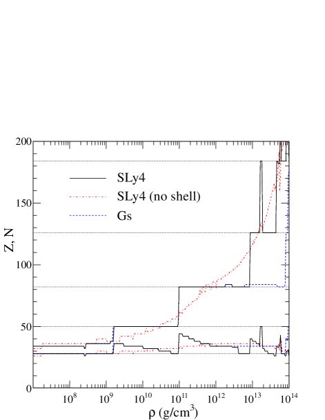
Figure 1: (Color online) The composition of the equilibrium neutron star crust as a function of density. Deviations originate primarily because of the symmetry energy: models where the symmetry energy depends more steeply with density have larger Z and smaller N, i.e. a composition closer to the valley of stability. The smoother curves labeled “no shell” do not include shell effects.

The free energy per baryon of matter in the full equilibrium is given in Figure 2. Note that the uncertainty in the homogenous matter EOS affects the free energy per baryon at higher densities even though the composition is not strongly affected.

Fig. 3 summarizes the properties of the accreted crust for the four EOSs used in this work. The entire crust is fixed at a temperature of T=$10^{8}$ K, and thermal effects do not strongly affect the composition. The initial composition is taken from Table I in Ref. Horowitz et al. (2007). The lower panel for each model shows the average neutron and proton numbers in the crust as a function of density along with an impurity parameter, $\left<Q\right>$. Given the average proton number,

$$\left<Z\right>=\left(\sum_{i}n_{i}Z_{i}\right)\left(\sum_{i}n_{i}\right)^{-1}\,,$$ (30)

the impurity parameter is defined as

$$\left<Q\right>=\left[\sum_{i}n_{i}\left(Z_{i}-\left<Z\right>\right)^{2}\right]\left[\sum_{i}n_{i}\right]^{-1}\,.$$ (31)

Generally, neutron numbers increase with density and proton numbers decrease with density, but a large amount of variation is present in the deepest regions in the crust. The dotted line in the upper panel is the chemical potential of the quasi-free neutrons in homogeneous matter at the same number density. The dashed line is the baryon chemical potential of the full equilibrium crust. The solid line is the full baryon chemical potential of matter in the accreted crust. The total amount of heating in the crust is equal to the baryon chemical potential (the Gibbs free energy per baryon). because a significant amount of heating occurs at densities slightly larger than the neutron drip density, the baryon chemical potential tends to form a valley at that density where heating overcomes the natural increase in baryon chemical potential from increasing pressure.

The dashed-dotted line is the sum of this baryon chemical potential with the total integrated heat from all the layers above the current one. This quantity from Fig. 5 of Ref. Haensel and Zdunik (2008) was defined to help explain the deep crustal heating phenomenon. The total amount of deep crustal heating is limited to the energy difference between this value and the baryon chemical potential in the full equilibrium crust. In models SLy4 and APR, the amount of deep crustal heat is limited by the rise of the baryon chemical potential in the full equilibrium crust. In models Gs and Rs, where the symmetry energy depends less strongly with density, the baryon chemical potential of the full equilibrium crust is smaller and thus the deep crustal heating is more significant.

Variations in the initial composition of matter are explored in the top part of Fig. 4. The left panel has an initial composition of pure ¹⁰⁶Pd and the right panel has an initial composition of pure ⁵⁶Ni. The final compositions in these models are not strikingly different from the X-ray burst ashes used in Fig. 3. The impurity parameters are much lower, except for a peak near $4\times 10^{12}$ g/cm³ in the ¹⁰⁶Pd case where the composition is recovering from the larger number of neutrons stored in nuclei in that case. Increasing the temperature to $10^{9}$ K, or varying the mass accretion rate (important for computing the relevant accretion timescale to compare with the fusion timescale) by an order of magnitude did not significantly change the results.

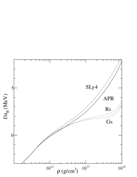
Figure 2: The energy per baryon of matter in the cold neutron star crust in full equilibrium. The distinction between the APR and SLy4 models and the Gs and Rs models is primarily due to the difference in the density dependence of the nuclear symmetry energy.

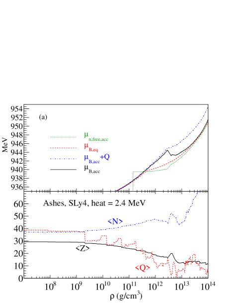
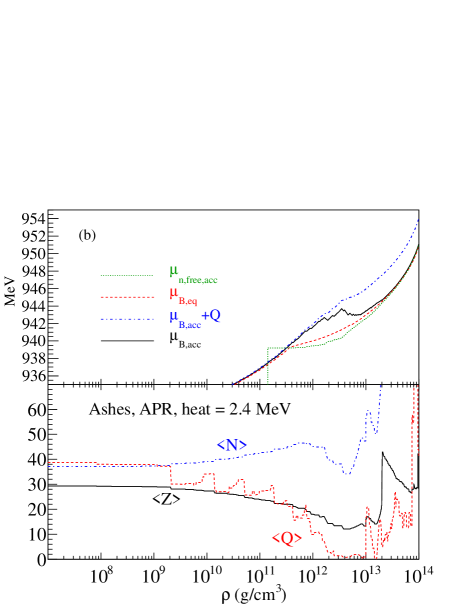
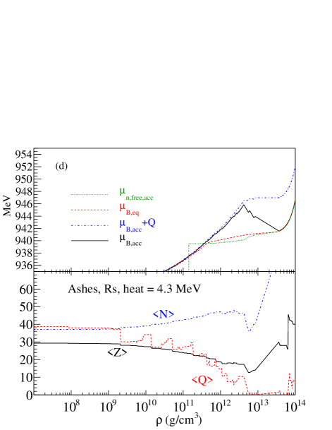
Figure 3: (Color online) The accreted crust properties for the four models used in this work: (a) SLy4, (b) APR, (c) Gs, and (d) Rs. X-ray burst ashes were used as the initial composition in each case. Each panel gives the total integrated heat generated by nuclear reactions throughout the crust.

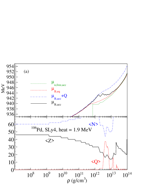
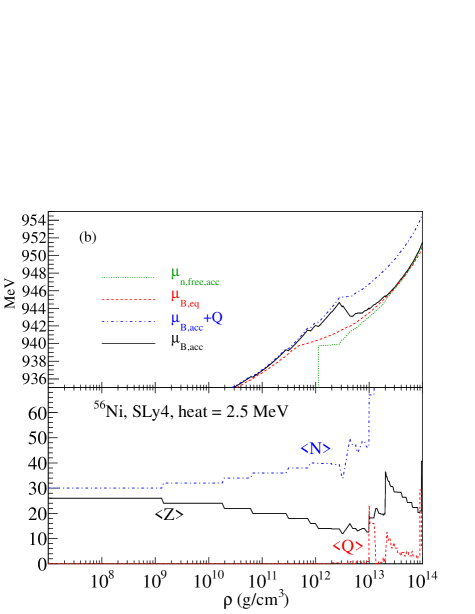
Figure 4: (Color online) The accreted crust properties for model SLy4 but using an initial composition of either pure ¹⁰⁶Pd (a) or pure ⁵⁶Ni (b). Each panel gives the total integrated heat generated by nuclear reactions throughout the crust.

The majority of the heating occurs through the emission of neutrons near neutron drip. This heating often occurs in large chains which effectively convert some nuclei entirely into neutrons, leaving the relative composition of the remaining nuclei unaltered. A sample chain of this form begins with two ⁴⁰Mg nuclei, both of which undergo 6 electron captures and enough neutron emissions to form ²²C. These two nuclei fuse to form one ⁴⁴Mg nucleus, which then may emit four neutrons to return to the original ⁴⁰Mg. This cycle effectively converts one nucleus entirely into neutrons. Only a fraction of nuclei can undergo such a cycle at any depth, and thus such cycles are difficult to resolve in single-nucleus models. While shell closures in this region are partially softened by the presence of the quasi-free neutron gas, resolving the nature of shell effects for neutron-rich nuclei in this region may be helpful in understanding the reaction pathway details at densities just higher than neutron drip.

IV Discussion

This work is an important tool to calibrate more sophisticated network calculations which follow the evolution of nuclei in the crust as they begin at the surface and evolve to lower depths. If the physical nucleon-nucleon interaction leads to a symmetry energy which depends more weakly with density, then this may result in more heating and will help alleviate the current difficulties that superburst models have in reproducing superburst data. Some of this additional heat, however, will be transmitted to the core rather than the crust, and a full simulation of the thermal profile which includes possible variation in the nuclear masses due to the symmetry energy is not yet available.

Compositional nonuniformity may also drive novel heating processes in the crust Medin and Cumming (2010a, b). While these heating processes are not included in the current model, they are also fundamentally limited by the difference in the baryon chemical potential between the accreted and equilibrium crusts.

The model outlined in this work ignores proton and light-fragment emission in accreting neutron stars, and may be incorrect near the crust-core phase transition. Near this density, protons may tunnel between nuclei and this will also affect the composition. Finally, the presence of pasta structures and nuclear structure uncertainties in the masses of nuclei are important in the deepest layers of the crust. The amount of heat generated at this depth is small, and the composition at the deepest regions in an accreting neutron star may be difficult to observe. The composition of the cold crust in equilibrium might be observable in the giant flares emitted by magnetars Steiner and Watts (2009).

A one-zone model may not properly estimate the properties of matter just near neutron drip. To demonstrate this, consider Fig. 5 of Ref. Haensel and Zdunik (2008). In the single-nucleus approximation, the baryon chemical potential, $\mu_{B}$, drops discontinuously as a function of the pressure at locations where the composition of the crust changes. This is clearly unphysical, as this means that the system can lower its energy by a finite amount by taking a neutron from pressures slightly lower than the drop in $\mu_{B}$ to pressures slightly larger than the drop. This means that neutrons might sink as they are emitted, and the crust will reconfigure itself to ensure that there are no strong discontinuities in $\mu_{B}$. (The electron chemical potential may also exhibit discontinuities in regions where multiple electron captures occur.) The multicomponent models in this work soften these discontinuities considerably, but a flow of neutrons cannot be ruled out in this one-zone model. A multi-zone generalization of this work is in progress.

V Acknowledgments:

The author thanks E.F. Brown, A. Cumming, R. Lau, S. Reddy, and H. Schatz for several useful discussions. This work was supported by DOE grant DE-FG02-00ER41132, NASA ATFP grant NNX08AG76G, and by the Joint Institute for Nuclear Astrophysics at MSU under NSF PHY grant 08-22648.

VI Appendix: Gibbs Free Energy Density

To compute the Gibbs free energy density, it is useful to compute the chemical potentials and entropies analytically from Eq. 17. An advantage of the liquid droplet model formalism is that these expressions are simple to compute accurately.

The global quasi-free neutron density is defined with ${\hat{n}}_{n}\equiv n_{n,\mathrm{out}}(1-\phi)$, and this (not $n_{n,\mathrm{out}}$ is the quantity directly connected to baryon number conservation. Thus, to compute the Gibbs energy the derivatives

$${\hat{\nu}}_{n}\equiv\left(\frac{\partial f}{\partial{\hat{n}}_{n}}\right)_{\{n_{i}\},T}$$ (32)

and

$$\nu_{i}\equiv\left(\frac{\partial f}{\partial n_{i}}\right)_{{\hat{n}}_{n},\{n_{j}\forall j\neq i\},T}\,$$ (33)

are required. The symbol $\nu$ is used rather than $\mu$ which is reserved for the chemical potentials in infinite matter

$$\mu_{n}\equiv\left[\frac{f_{\infty}(n_{n,\mathrm{out}},T)}{\partial n_{n,\mathrm{out}}}\right]_{T}\,,\quad\mathrm{and}$$

$$\mu_{e}\equiv\left[\frac{f_{\mathrm{elec}}(n_{e},T)}{\partial n_{e}}\right]_{T}\,.$$ (34)

Note that these chemical potentials are defined including the rest mass energy. To be more concise, the subscripts will sometimes be suppressed in the following. The Gibbs free energy density is then

$$g={\hat{\nu}}_{n}{\hat{n}}_{n}+\sum_{i}\nu_{i}n_{i}\,.$$ (35)

It is useful to note that $n_{n,\mathrm{in},i}=n_{n,\mathrm{in},i}(\chi_{i})$ is distinct quantity for each nuclear species $i$ and is a function of $\chi_{i}$. For simplicity, this is denoted as $n_{ni}$ below. Also note that no separate term in the Gibbs free energy is required for the electrons since their number density is not an independent variable. In this section, it is also easier to think of the function ${\cal E}_{\mathrm{nuc}}$ as a set of functions of the form ${\cal E}_{\mathrm{nuc},i}(n_{n,\mathrm{out}},\chi_{i})$. For each nucleus $i$,

$$N_{i}n_{e}=N_{i}\left(\sum_{j}n_{j}Z_{j}\right)=Z_{i}\chi_{i}n_{ni}$$ (36)

and this implies that $\chi$ and $n_{e}$ both depend only on the number densities of nuclei and not separately on $n_{n,\mathrm{out}}$. From Eq. 36, one can obtain the relation $\partial n_{e}/\partial n_{i}=Z_{i}$ and the derivative

$$\left(\frac{\partial\chi_{j}}{\partial n_{i}}\right)_{\{n_{j}\}\forall j\neq i,~{}{\hat{n}}_{n}}=\frac{N_{j}Z_{i}}{Z_{j}n_{nj}+Z_{j}\chi_{j}g^{\prime}(\chi_{j})}\,.$$ (37)

This derivative is non-zero for $i\neq j$ because the nuclei are all coupled by the Coulomb interaction through the electron density. Some simplification is afforded by the relation $\phi_{i}=N_{i}n_{i}/n_{ni}$, where $n_{ni}$ depends only on $\chi_{i}$, which shows that $\phi_{i}$ is constant when all of the $\{n_{i}\}$ are held fixed. Thus,

$$\left(\frac{\partial n_{n,\mathrm{out}}}{\partial{\hat{n}}_{n}}\right)_{\{n_{i}\}}=(1-\phi)^{-1}$$ (38)

and

$$\left(\frac{\partial n_{n,\mathrm{out}}}{\partial n_{i}}\right)_{\{n_{j}\}\forall j\neq i,~{}{\hat{n}}_{n}}=\frac{{\hat{n}}_{n}}{\left(1-\phi\right)^{2}}\sum_{j}\left(\frac{\partial\phi_{j}}{\partial n_{i}}\right)$$ (39)

One can rewrite the derivative of $\phi_{j}$ in terms of the derivative of $\chi_{j}$ determined above

$$\left(\frac{\partial\phi_{j}}{\partial n_{i}}\right)_{\{n_{j}\}\forall j\neq i,~{}{\hat{n}}_{n}}=\frac{N_{j}}{n_{nj}}\left[\delta_{ij}-\frac{n_{j}g^{\prime}(\chi_{j})}{n_{nj}}\left(\frac{\partial\chi_{j}}{\partial n_{i}}\right)_{{\hat{n}}_{n}}\right]\,$$ (40)

where $\delta_{ij}$ is 1 if $i=j$ and zero otherwise. The last derivative which is required is

$$\left(\frac{\partial N_{j}^{\prime}}{\partial n_{i}}\right)_{\{n_{j}\}\forall j\neq i,~{}{\hat{n}}_{n}} = -4\pi R_{\mathrm{n},j}^{2}\left[\frac{R_{\mathrm{n},j}}{3}\left(\frac{\partial n_{n,\mathrm{out}}}{\partial n_{i}}\right)\right.$$ (41)

$$\left.+n_{n,\mathrm{out}}\left(\frac{\partial R_{\mathrm{n},j}}{\partial\chi_{j}}\right)\left(\frac{\partial\chi_{j}}{\partial n_{i}}\right)\right]\,.$$

The derivative of $f$ with respect to ${\hat{n}}_{n}$ is

$${\hat{\nu}}_{n} = \left(\frac{\partial n_{n,\mathrm{out}}}{\partial{\hat{n}}_{n}}\right)\left\{\mu_{n}+\sum_{i}n_{i}\left[\left(\frac{\partial{\cal E}_{\mathrm{nuc},i}}{\partial n_{n,\mathrm{out}}}\right)_{\chi_{i}}+\right.\right.$$ (42)

$$\left.\left.-\frac{4\pi}{3}R_{n,i}^{3}m_{n}\right]\right\}\,.$$

Note that this implies

$${\hat{n}}_{n}~{}\nu_{{\hat{n}}_{n}}=n_{n,\mathrm{out}}\left(\frac{\partial f}{\partial n_{n,\mathrm{out}}}\right)_{\{n_{i}\}}\,.$$ (43)

The derivative of $f$ with respect to the number density of nucleus $i$ is

$$\nu_{i} = \left(\frac{\partial f}{\partial n_{n,\mathrm{out}}}\right)\left(\frac{\partial n_{n,\mathrm{out}}}{\partial n_{i}}\right)+Z_{i}\mu_{e}+{\cal E}_{\mathrm{nuc},i}+Z_{i}m_{p}$$ (44)

$$+N_{i}^{\prime}m_{n}+\sum_{j}n_{j}h_{ij}$$

where $h_{ij}$ is defined by

$$h_{ij} \equiv \left(\frac{\partial{\cal E}_{\mathrm{nuc},j}}{\partial\chi_{j}}\right)_{n_{n,\mathrm{out}}}\left(\frac{\partial\chi_{j}}{\partial n_{i}}\right)$$ (45)

$$+\left(\frac{\partial{\cal E}_{\mathrm{nuc},j}}{\partial n_{n,\mathrm{out}}}\right)_{\chi_{j}}\left(\frac{\partial n_{n,\mathrm{out}}}{\partial n_{i}}\right)+m_{n}\left(\frac{\partial N_{j}^{\prime}}{\partial n_{j}}\right)_{n_{n,\mathrm{out}}}$$

References

- Schatz et al. (1998) H. Schatz, A. Aprahamian, J. Görres, M. Wiescher, T. Rauscher, J. F. Rembges, F.-K. Thielemann, B. Pfeiffer, P. Möller, K.-L. Kratz, et al., Phys. Rep. 294, 167 (1998).
- Haensel and Zdunik (1990) P. Haensel and J. L. Zdunik, Astron. & Astrophys. 227, 431 (1990).
- Brown et al. (1998) E. F. Brown, L. Bildsten, and R. E. Rutledge, Astrophys. J. Lett. 504, L95 (1998).
- Shternin et al. (2007) P. S. Shternin, D. G. Yakovlev, P. Haensel, and A. Y. Potekhin, Mon. Not. Royal Astron. Soc. 382, L43 (2007).
- Brown and Cumming (2009) E. F. Brown and A. Cumming, Astrophys. J. 698, 1020 (2009).
- Heinke et al. (2006) C. O. Heinke, G. B. Rybicki, R. Narayan, and J. E. Gridlay, Astrophys. J. 644, 1090 (2006).
- Yakovlev and Pethick (2004) D. G. Yakovlev and C. J. Pethick, Ann. Rev. Astron. Astrophys. 42, 169 (2004).
- Page et al. (2004) D. Page, J. M. Lattimer, M. Prakash, and A. W. Steiner, Astrophys. J. Supp. 155, 623 (2004).
- Page et al. (2009) D. Page, J. M. Lattimer, M. Prakash, and A. W. Steiner, Astrophys. J. 707, 1131 (2009).
- Cumming and Bildsten (2001) A. Cumming and L. Bildsten, Astrophys. J. 559, L127 (2001), eprint astro-ph/0107213.
- Strohmayer and Brown (2002) T. E. Strohmayer and E. F. Brown, Astrophys. J. 566, 1045 (2002).
- Brown (2004) E. F. Brown, Astrophys. J. Lett. 614, 57 (2004).
- Cumming et al. (2006) A. Cumming, J. Macbeth, J. J. M. in ’t Zand, and D. Page, Astrophys. J. 646, 429 (2006).
- Gupta et al. (2007) S. Gupta, E. F. Brown, H. Schatz, P. Möller, and K.-L. Kratz, Astrophys. J. 662, 1188 (2007).
- Cooper et al. (2009) R. L. Cooper, A. W. Steiner, and E. F. Brown, Astrophys. J. 702, 660 (2009).
- Woosley et al. (2004) S. E. Woosley, A. Heger, A. Cumming, R. D. Hoffman, J. Pruet, T. Rauscher, J. L. Fisker, H. Schatz, B. A. Brown, and M. Wiescher, Astrophys. J. Supp. 151, 75 (2004).
- Gupta et al. (2008) S. S. Gupta, T. Kawano, and P. Möller, Phys. Rev. Lett. 101, 231101 (2008).
- Horowitz et al. (2007) C. J. Horowitz, D. K. Berry, and E. F. Brown, Phys. Rev. E 75, 066101 (2007).
- Horowitz et al. (2009) C. J. Horowitz, O. L. Caballero, and D. K. Berry, Phys. Rev. E 79, 026103 (2009).
- Horowitz and Berry (2009) C. J. Horowitz and D. K. Berry, Phys. Rev. C 79, 065803 (2009).
- Skyrme (1959) T. H. R. Skyrme, Nucl. Phys. 9, 615 (1959).
- Akmal et al. (1998) A. Akmal, V. R. Pandharipande, and D. G. Ravenhall, Phys. Rev. C 58, 1804 (1998).
- Chabanat (1995) E. Chabanat, Ph. D. Thesis, University of Lyon (1995).
- Friedrich and Reinhard (1986) J. Friedrich and P.-G. Reinhard, Phys. Rev. C 33, 335 (1986).
- Oyamatsu and Iida (2007) K. Oyamatsu and K. Iida, Phys. Rev. C 75, 015801 (2007).
- Steiner (2008) A. W. Steiner, Phys. Rev. C 77, 035805 (2008).
- Newton et al. (2011) W. G. Newton, M. Gearhart, and B.-A. Li, arXiv:1110.4043 (2011).
- Lattimer et al. (1985) J. M. Lattimer, C. J. Pethick, D. G. Ravenhall, and D. Q. Lamb, Nucl. Phys. A 432, 646 (1985).
- Ravenhall et al. (1983) D. G. Ravenhall, C. J. Pethick, and J. R. Wilson, Phys. Rev. Lett. 50, 2066 (1983).
- Dieperink and van Isacker (2009) A. E. L. Dieperink and P. van Isacker, European Physical Journal A 42, 269 (2009).
- Grasso et al. (2008) M. Grasso, E. Khan, J. Margueron, and N. Van Giai, Nucl. Phys. A 807, 1 (2008).
- Denisov (2005) V. Y. Denisov, Phys. of At. Nucl. 68, 1133 (2005).
- Audi et al. (2003) G. Audi, A. H. Wapstra, and C. Thibault, Nucl. Phys. A 729, 337 (2003).
- Souza et al. (2009) S. R. Souza, A. W. Steiner, W. G. Lynch, R. Donangelo, and M. A. Famiano, Astrophys. J. 707, 1495 (2009), eprint 0810.0963.
- Bonche et al. (1984) P. Bonche, S. Levit, and D. Vautherin, Nucl. Phys. A 427, 278 (1984).
- Suraud (1987) E. Suraud, Nucl. Phys. A 462, 109 (1987).
- Lattimer and Swesty (1991) J. M. Lattimer and F. D. Swesty, Nucl. Phys. A 535, 331 (1991).
- Hix et al. (2003) W. R. Hix, O. E. B. Messer, A. Mezzacappa, M. Liebendörfer, J. Sampaio, K. Langanke, D. J. Dean, and G. Martinez-Pinedo, Phys. Rev. Lett. 91, 201102 (2003).
- Botvina and Mishustin (2005) A. S. Botvina and I. N. Mishustin, Phys. Rev. C 72, 048801 (2005).
- Sumiyoshi and Röpke (2008) K. Sumiyoshi and G. Röpke, Phys. Rev. C 77, 055804 (2008).
- Arcones et al. (2008) A. Arcones, G. Martinez-Pinedo, E. O’Connor, A. Schwenk, H.-T. Janka, C. J. Horowitz, and K. Langanke, Phys. Rev. C 78, 015806 (2008).
- Hempel and Schaffner-Bielich (2010) M. Hempel and J. Schaffner-Bielich, Nucl. Phys. A 837, 210 (2010).
- Haensel and Zdunik (2008) P. Haensel and J. L. Zdunik, Astron. & Astrophys. 480, 459 (2008).
- Fowler and Hoyle (1964) F. A. Fowler and F. Hoyle, Astrophys. J. Suppl. 9, 201 (1964).
- Beard et al. (2010) M. Beard, A. V. Afanasjev, L. C. Chamon, L. R. Gasques, M. Wiescher, and D. G. Yakovlev, arXiv.org:1002.0741 (2010).
- Yakovlev et al. (2006) D. G. Yakovlev, L. R. Gasques, M. Beard, M. Wiescher, and A. V. Afanasjev, Phys. Rev. C 74, 035803 (2006).
- Medin and Cumming (2010a) Z. Medin and A. Cumming, Phys. Rev. E 81, 036107 (2010a).
- Medin and Cumming (2010b) Z. Medin and A. Cumming, Astrophys. J 730, 97 (2010b).
- Steiner and Watts (2009) A. W. Steiner and A. L. Watts, Phys. Rev. Lett. 103, 181101 (2009).