Gravitational wave background from population III binaries

Abstract

Context. Current star formation models imply that the binary fraction of population III stars is non-zero. The evolution of these binaries must have led to the formation of compact object binaries.

Aims. We estimate the gravitational wave background originating in these binaries and discuss its observability .

Methods. The properties of the population III binaries are investigated using a binary population synthesis code. We numerically model the background and take into account the evolution of eccentric binaries.

Results. The gravitational wave background from population III binaries dominates the spectrum below 100 Hz. If the binary fraction is larger than $10^{-2}$, the background will be detectable by Einstein Telescope (ET), Laser Interferometer Space Antenna (LISA) and DECi-Hertz Interferometer Gravitational wave Observatory (DECIGO).

Conclusions. The gravitational wave background from population III binaries will dominate the spectrum below 100 Hz. The instruments LISA, ET and DECIGO should either see it easily or, in the case of non-detection, provide very strong constraints on the properties of the population III stars.

1 Introduction

Coalescing compact object binaries are among the best candidates for sources of gravitational waves. They include the double neutron star binaries (DNS), the mixed, black hole neutron star binaries (BHNS) and binary black holes (BBH). A gravitational wave signal may be detected as single events from nearby sources, but the signals of more distant objects will overlap contributing to the gravitational wave background (GWB). The GWB from coalescing compact object binaries has been investigated by numerous authors (e.g., Tumlinson & Shull 2000; Bromm et al. 2001; Rosado 2011; Zhu et al. 2011; Olmez et al. 2011; Regimbau 2011; Marassi et al. 2011). Existing gravitational wave detectors Laser Interferometer Gravitational Wave Observatory (LIGO) and Virgo Gravitational Wave Detector have achieved their design sensitivity (Accadia et al. (2011), Kawabe & the LIGO Collaboration (2008)), and are currently undergoing transitions to the advanced phase with a sensitivity increase of a factor 30. Additionally, there are plans to construct other large-scale detectors such as Large-scale Cryogenic Gravitational wave Telescope (LCGT) (Kuroda & LCGT Collaboration 2010). In the more distant future, third generation detectors such as the Einstein Telescope (ET) (Van Den Broeck 2010) should be constructed. Theses instrumental developments ensure that the investigation of the stochastic backgrounds of gravitational waves is very important. At lower frequencies such as designed band of ET ($\sim$ 1Hz), we expect large populations of distant object to be observed. The biggest contribution in that frequency window will come from massive BBH. There are no direct observations of this kind of objects, hence there are many uncertainties in the stellar evolution models of the formation of BBH. Because of the high redsift range of future detectors, there is a possibility that among observed objects there could be the remnants of the oldest stars in the Universe. Population III stars should be metal free, thus they should produce black holes of masses reaching hundreds of solar masses. If our understanding of their evolution is correct, there should be a significant gravitational background from remnants of population III stars.

In this paper, we investigate the possible contribution to the GWB of population III star binaries. Population III stars are the first stars in the Universe that formed out of metal-free material. As such, they had very different properties from the currently forming stars. The evolution and properties of single population III stars were investigated by Baraffe et al. (2001) and Tan (2008), who found that single population III stars are stable up to a few hundred of solar masses. Moreover, they evolve with little mass loss. The evolution of this massive star will end up either in a pair instability supernova leaving no remnant, or forming a black hole through a direct collapse. While no population III stars are known, their properties have been investigated by numerical simulations of the collapse of metal-free clouds of gas. These simulations have shown that the initial mass function of a population III star is skewed towards higher masses than those of either population I or II stars (Abel et al. 2002; Bromm et al. 2002). The existence of binaries among population III stars has been uncertain, although simulations of the collapse of rotating clouds of gas have found evidence of bar instabilities and the formation of two protostars (Saigo et al. 2004; Machida et al. 2008). Since all known stellar populations contain a significant fraction of binaries, it seems justified to consider the properties of population III binaries. The evolution of population III binaries was investigated by Belczynski et al. (2004) and Kulczycki et al. (2006). They found that the coalescence of BBH binaries originating in population III stars may be a significant source of gravitational waves detectable by the current and future gravitational wave interferometers. In section 2, we analyze the gravitational wave spectrum of eccentric binaries, and section 3 is devoted to the analysis of properties of population III binaries. Section 4 contains an outline of the estimate of the GWB. We present the results in section 5, and in section 6 we discuss them.

2 Population of stars - models

The evolution of population III metal-free stars was first examined in detail about ten years ago by Heger et al. (2001), Baraffe et al. (2001), Marigo et al. (2001), Marigo et al. (2003), and Schaerer (2002). These stars were found to be stable with masses of up to 500 $\textrm{M}_{\odot}$. Population III star evolve very quickly experiencing nearly no mass loss. Depending on their initial mass, they may form neutrons stars, black holes, or leave no remnant at all, because of total star disruption in pair instability supernovae (Heger & Woosley 2002). The mass spectrum of population III stars is still a matter of debate. On the one hand the simulations of metal-free cloud collapse have clearly illustrated the possibility of forming high mass objects. Searches for the low mass metal-free stars that are predicted to persist in the Universe have brought no success, which indicates that the low mass cutoff of the population III initial mass function was significantly higher than for the current population of stars. An additional question is whether population III stars were also formed as binaries. Every known stellar population contains a significant fraction of binaries, so one should also expect this to be the case for population III stars. Numerical simulations of the collapse of rotating metal-free clouds indicate the appearance of a bar instability leading to the formation of two protostars in a binary (Saigo et al. 2004). In recent simulations (Turk et al. 2009; Stacy et al. 2010; Greif et al. 2011; Clark et al. 2011; Stacy et al. 2012), a similar result was shown. A massive protostellar cloud develops spiral structure, instabilities, and leads to the formation of several multiple systems. Thus, we conclude that there is ample justification to investigate population III binary evolution and its consequences.

We model the evolution of population III binaries using a code described in Belczynski et al. (2004). The code uses the evolutionary sequences based on Heger et al. (2001), Baraffe et al. (2001), and Marigo et al. (2001). It includes a detailed treatment of the calculation of stellar remnants. The binary evolution calculation involves the analysis of the stability of mass transfers. The common envelope mass transfers end in a merger if the donor is a main sequence star, and for giant stars we use the standard formalism of Webbink (1984).

We assumed that the initial mass function of the primaries stretches between 10 $\textrm{M}_{\odot}$ and 500 $\textrm{M}_{\odot}$ with the exponent of -2.35. The mass ratio is drawn from a flat distribution. The initial orbital separation distribution is flat as a logarithm of $a$. The range of initial orbital separations is bounded from below by the requirement that the stars are not in contact at the zero age main sequence (ZAMS) - $a_{min}=1.3(R_{1}+R_{2})$. The upper bound is more arbitrary. We chose $a_{max}=10^{6}R_{\odot}$. While Bromm & Loeb (2006) argue that the upper limit to the initial separation is as large as $5\times 10^{7}R_{\odot}$, we wished to include all systems that interact. The binaries with initial separations close to or above our upper limit will not interact and if they survive the evolution and form compact object binaries, they will only contribute to the GW background spectrum below $10^{-11}$Hz. The uncertainty in the number of binaries due to a variation in the upper cutoff $a_{max}$ is small because of the logarithmic distribution of initial orbital separations. We calculated the evolution of binaries and note that the cases when a compact object binary was formed. We then traced its evolution due to the emission of gravitational waves.

2.1 Properties of compact objects

We tracked the evolution of $10^{6}$ binary stars of zero metallicity using the population synthesis code StarTrack. As a result, we obtained 462496 compact objects, which we treat as a realistic sample of population III remnants. More than 60% of them are BBH systems, where both components have masses greater than $2.5\textrm{M}_{\odot}$. Detailed distributions of initial parameters are presented in Figure 1. In the top panel, one can see that there is very broad range of initial eccentricities - over 60% of all binaries have eccentricities greater than $0.1$. The bottom panel shows the distributions of chirp masses and coalescence times. Only 12% of binaries will merge within the present Hubble time.

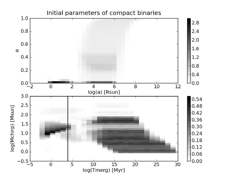
Figure 1: The initial properties of the population III compact object binaries. The top panel shows the distribution of the orbital properties, i.e. the density in the plane spanned by the semi-major axis and the eccentricity of the orbit. The lower panel shows the distribution of the chirp masses and the merger times of the binaries. Vertical line represents the Hubble time. Numbers represent the percentage of all binaries in the simulation.

3 Gravitational wave spectrum of eccentric binaries

While the spectra of circular binaries have been well-studied, we have shown above that a large fraction of population III binaries will be eccentric. It is therefore important to investigate the possible effects of eccentricity on the gravitational wave spectra of compact object binaries. (Peters & Mathews 1963; Peters 1964)

3.1 General derivation

The gravitational wave spectrum from a binary can be calculated as

$$\frac{dE_{gw}}{df_{gw}}=\frac{dE_{gw}}{dt}\left(\frac{df_{gw}}{dt}\right)^{-1}.$$ (1)

The velocity on an eccentric orbit changes over its period, hence the instantaneous orbital frequency also varies. Thus, the system is radiating across some range of frequencies, not only one in particular, as in the case of a circular orbit.

In the quadrupole approximation, the orbit decays owing to gravitational wave emission and the orbital parameters change as

$$\frac{da}{dt} = -\frac{64}{5}\frac{G^{3}\mu M^{2}}{a^{3}c^{5}}\Psi(e),$$ (2)

$$\Psi(e) = \frac{1+73/24e^{2}+37/96e^{4}}{(1-e^{2})^{7/2}},$$ (3)

while orbital frequency is

$$f_{orb}={1\over 2\pi}\left({GM\over a^{3}}\right)^{1/2},$$ (4)

where we have denoted the total mass of the binary $M$, $\mu$ is the reduced mass, and $a$ is the semi-major axis. An eccentric binary emits gravitational waves in a spectrum of harmonics of the orbital frequency

$$f^{n}_{gw}=nf_{orb},$$ (5)

$$\frac{df_{gw}}{dt}=n\frac{df_{orb}}{dt}.$$ (6)

In the case of a circular orbit, gravitational waves are emitted in only one mode $n=2$. Inserting Eq. 4 and Eq. 2 into Eq. 6, we obtain

$$\frac{df^{n}_{gw}}{dt}=\frac{96}{5}\left(\frac{2\pi}{n}\right)^{8/3}\frac{{f^{n}_{gw}}^{11/3}G^{5/3}M_{chirp}^{5/3}}{c^{5}}\Psi(e),$$ (7)

where we have introduced the chirp mass, which is a quantity that determines the amplitude and frequency dependence of the inspiral gravitational wave signal $M_{chirp}=\mu^{3/5}M^{2/5}$. The power of the radiation for each harmonic was calculated by Peters & Mathews (1963) to be

$$\frac{dE}{dt}(n)=\frac{32}{5}\frac{G^{4}\mu^{2}M^{3}}{c^{5}a^{5}}g(n,e),$$ (8)

where $g(n,e)$ is

$$g(n,e) = \frac{n^{4}}{32}\left\{[J_{n-2}(ne)-2eJ_{n-1}(ne)+\frac{2}{n}J_{n}(ne)\right.$$ (9)

$$+2eJ_{n+1}(ne)-J_{n+2}(ne)]^{2}$$

$$+(1-e^{2})\left[J_{n-2}(ne)-2J_{n}(ne)+J_{n+2}(ne)\right]^{2}$$

$$\left.+\frac{4}{3n^{2}}\left[J_{n}(ne)\right]^{2}\right\}$$

and $J_{n}$ are the Bessel functions. This result follows from the Fourier analysis of the Kepler motion Peters & Mathews (1963). We obtain the instantaneous spectrum of gravitational waves from an eccentric binary by combining Eq. 1- 8 and Eq. 7

$$\frac{dE}{df^{n}_{gw}}=\frac{\pi}{3}\frac{1}{G}\left(\frac{4}{n^{2}}\right)^{1/3}\frac{\left(GM_{chirp}\right)^{5/3}}{\left(f^{n}_{gw}\pi\right)^{1/3}}\frac{g(n,e)}{\Psi(e)}.$$ (10)

For a circular orbit this reduces to the well-known result, e.g. (Phinney 2001)

$$\frac{dE}{df_{gw}}\Bigg{|}_{e=0}=\frac{\pi}{3}\frac{1}{G}\frac{\left(GM_{chirp}\right)^{5/3}}{\left(f_{gw}\pi\right)^{1/3}},$$ (11)

since $\Psi(e=0)=1$, $g(n,e=0)=1$ when $n=2$ and $g(n\neq 2,e=0)=0$. The result has to be averaged over the lifetime of the binary. In the following section, we discuss two cases: the long-lived and the short-lived binaries, as outlined below.

3.2 Long-lived systems

By the term long-living, we mean that the time to coalescence is longer than the present Hubble time, which we assume for simplicity to be $t_{H}=10^{4}Myr$. We are interested in objects that have not merged. These objects have very wide orbits and the semi-major axis of the binary, as well as its eccentricity, can be assumed to be constant during the entire evolution time. The spectrum is then discrete as the binary emits the gravitational radiation only at the frequencies specified by the harmonics

$$\frac{dE}{df}=\sum_{n=2}^{\infty}\delta(f-nf_{orb})\frac{dE}{df^{n}_{gw}},$$ (12)

where the spectrum in each harmonic is given by Eq. 10.

To illustrate this case, we chose a binary consisting of two massive black holes of masses $M_{1}=M_{2}=300\,M_{\odot}$ on a wide orbit $a=1.2\times 10^{6}\,R_{\odot}$. We present the spectra for a few values of the eccentricity in Figure 2.

Figure 2: Spectra of the GW radiation from a long-living binary ($M_{1}=M_{2}=300\,M_{\odot}$, $a=1.2\times 10^{6}\,R_{\odot}$) for different values of eccentricity. A single ’plus’ mark corresponds to a circular orbit, by crosses we show the case for eccentricity 0.5, stars corresponds to eccentricity 0.7, and squares to initial eccentricity 0.9.

When the eccentricity is almost zero, we have just one point,which corresponds to a very wide, circular orbit. The velocity is then constant and we observe only one frequency. As the eccentricity increases, we observe that spectrum becomes wider. In addition, the maximum of the energy distribution is shifted to higher frequencies. For the highest considered eccentricity (0.9), there is a minimum around a frequency $10^{-11}$, which is caused by the specific structure of the function described by Eq. 9.

3.3 Short-lived systems

In this group, we consider systems that can coalescence during their evolution. The orbit changes and we observe radiation across a very wide range of frequencies. The binary emits a continous spectrum over its lifetime. The orbital frequency changes from $f_{ini}$, which is the initial orbital frequency determined by the orbital parameters after formation of the second compact object in the binary, to the final orbital frequency just before merger. For the final orbital frequency, we chose the frequency for the marginally stable orbit

$$f_{ISCO}=\frac{c^{3}}{6\sqrt{6}\pi G(M_{1}+M_{2})}.$$ (13)

As the binary evolves, its eccentricity decreases and its evolution of eccentricity can be found by solving the equation

$$\frac{de}{df_{orb}}=-\frac{19}{18}\frac{1}{f_{orb}}\frac{e}{(1-e^{2})^{5/2}}\left(1+\frac{121}{304}e^{2}\right).$$ (14)

Denote the dependence of the eccentricity on the orbital frequency as $e(f_{orb})$.

The gravitational wave spectrum is

$$\frac{dE}{df}=\sum_{n=2}^{\infty}\frac{dE}{df^{n}_{gw}}(e=e(f^{n}_{gw}/n)),$$ (15)

where the functions $\frac{dE}{df^{n}_{gw}}$ are evaluated only for the frequencies in the range $nf_{ini}<f^{n}_{gw}<nf_{ISCO}$.

We illustrate this case with a binary of the same mass as in previous section of $M_{1}=M_{2}=300\,M_{\odot}$, but on a much tighter orbit $a=1.2\times 10^{2}\,R_{\odot}$. We present the spectra for four different values of eccentricity in Figure 3.

Figure 3: Spectrum of the GW radiation from short-lived binaries for different values of the initial eccentricity. Solid line corresponds to circular orbit, by dashed line we show case for eccentricity 0.5, dotted line corresponds to eccentricity 0.7 and dash-dotted line to initial eccentricity 0.9

For zero eccentricity, the spectrum is a simple power law. For non-zero eccentricities, the power law spectrum acquires a tail that increases to higher frequencies. The shape of the high frequency tail in the spectrum is determined by the eccentricity of the system.

4 Gravitational wave background radiation

We analyze the population of massive black hole binaries using the StarTrack population synthesis code (Belczynski et al. 2002). For each system, we obtain its component masses $M_{1,i}$, $M_{2,i}$, and its initial orbital parameters: the semi-major axis $a_{i}$, and the eccentricity $e_{i}$. We denote the total mass of the system as $M_{i}=M_{1,i}+M_{2,i}$ , the reduced mass as $\mu_{i}=\frac{M_{1,i}M_{2,i}}{M_{1,i}+M_{2,i}}$, and the chirp mass $M_{chirp,i}=\mu_{i}^{3/5}M_{i}^{2/5}$.

4.1 Evolution of the orbit

The initial value of the semi-major axis is given by the synthesis population code and we can use it to estimate the lowest frequency possible for any particular binary

$$f_{i,1}=\sqrt{\frac{GM}{\pi^{2}a_{i}^{3}}}.$$ (16)

The eccentricity and semi-major axis changes during the evolution according to the two differential equations

$$\frac{da}{dt}=-\frac{\beta}{a^{3}}\Psi(e)\hskip 42.67912pt\Psi(e)=\frac{1+73/24e^{2}+37/96e^{4}}{(1-e^{2})^{7/2}},$$ (17)

$$\frac{de}{dt}=-\frac{19}{12}\frac{\beta}{a^{4}}\Phi(e)\hskip 42.67912pt\Phi(e)=\frac{(1+121/304e^{2})e}{(1-e^{2})^{5/2}}.$$ (18)

We have to calculate the size of the orbit after a Hubble time. For short-living systems, we assume that the final great semi-major axis is $a_{f}=10^{-3}R_{\odot}$, beyond which we should consider tidal effects. The angular momentum timescale is comparable to age of the binary, hence the system will merge eventually. For long-living systems, we have to solve Eq. (17) and Eq. (18). We can then calculate the frequency corresponding to the final size of the orbit in the same way as we did it for initial parameters.

Figure 4: The gravitational wave background from population III stars. The standard model results are presented as the thick solid line and denoted as A. The thin lines are labeled with a letter denoting the model; for a description, see Table 1. We also present the sensitivities of future gravitational wave experiments. Bottom panel was created for clarity, because the models G, F1, and F2 are no different from the standard model.

4.2 Spectrum

A stochastic background is described in terms of the present-day gravitational wave energy density ($\rho_{gw}$) per logarithmic frequency interval normalized to the critical rest-mass energy density ($\rho_{c}c^{2}$) Phinney (2001)

$$\Omega_{gw}(f)=\frac{1}{\rho_{c}c^{2}}\frac{d\rho_{gw}(f)}{d\ln(f)}.$$ (19)

The total present-day energy density contained in the gravitational radiation is related to $\Omega(f)$ and the amplitude of the gravitational wave spectrum over a logarithmic frequency interval ($h_{c}(f)$) through

$$\mathcal{E}_{gw}=\int_{0}^{\infty}\rho_{c}c^{2}\Omega_{gw}(f)\frac{df}{f}=\int_{0}^{\infty}\frac{\pi}{4}\frac{c^{2}}{G}f^{2}h_{c}^{2}(f)\frac{df}{f}.$$ (20)

On the other hand, $\mathcal{E}_{gw}$ should be the sum of the energy radiated by all sources at all redshifts

$$\mathcal{E}_{gw}=\int_{0}^{\infty}\int_{0}^{\infty}N(z)\frac{1}{1+z}f_{r}\frac{dE_{gw}}{df_{r}}dz\frac{df}{f}.$$ (21)

Since the Universe is expanding, the observed frequency is different from the emitted one and equal to $f_{r}=f(1+z)$, while $N(z)$ is the number of sources in the interval $(z,z+1)$.

Combining (20) and (21), we obtain

$$\rho_{c}c^{2}\Omega_{gw}(f) = \frac{\pi}{4}\frac{c^{2}}{G}f^{2}h_{c}^{2}(f)=$$

$$= \int_{0}^{\infty}N(z)\frac{1}{1+z}\left(f_{r}\frac{dE_{gw}}{df_{r}}\right)\Bigg{|}_{f_{r}=f(1+z)}dz.$$

Using Eq. (10), we obtain equations describing the spectrum from a single harmonic for one type of source

$$\Omega(f_{gw}^{n}) = \frac{G^{2/3}M_{chirp}^{5/3}2^{2/3}\pi^{2/3}}{3n^{2/3}\rho_{c}c^{2}}\times$$

$$\times(f_{gw}^{n})^{2/3}\frac{g(n,e)}{\Psi(e)}N_{0}\left<(1+z)^{-1/3}\right>,$$

where $N_{0}$ is the density of one type of sources

$$N_{0}=\frac{1}{N_{tot}}f_{bin}n_{pop3},\qquad f_{bin}=\frac{2}{1+\frac{1}{f_{b}}}.$$ (24)

The term in the brackets is

$$\left<(1+z)^{-1/3}\right>=\frac{1}{N_{0}}\int_{z_{min}}^{z_{max}}\frac{N(z)}{(1+z)^{1/3}}dz.$$ (25)

In the case of population III binaries, the right-hand side integral is trivial, since we assumed that all population III stars were formed at single redshift $z=15$. Taking into account the very short evolution timescales of massive stars population III stars, we were able to assume that the binary compact objects were formed at the same redshift.

To obtain the energy density from all simulated objects, we sum over harmonics (index $n$) and over the total number of binaries (index $i$)

$$\Omega(f) = \sum_{i=1}^{N}\sum_{n=2}^{\infty}\delta(f-f_{i}^{n})\frac{G^{2/3}M_{chirp,i}^{5/3}2^{2/3}\pi^{2/3}}{3n^{2/3}\rho_{c}c^{2}}\times$$

$$\times(f_{i}^{n})^{2/3}\frac{g(n,e)}{\Psi(e)}N_{0}\left<(1+z)^{-1/3}\right>.$$

The amplitude of the gravitational wave spectrum ($h_{c}(f)$) and the spectral density of the gravitational wave background ($S(f)$) are given by

$$h_{c}^{2}(f)=\frac{4\rho_{c}G}{\pi f^{2}}\Omega(f) S(f)=\frac{h_{c}}{f}.$$ (27)

5 Results

We present the resulting gravitational wave background spectrum in Figure 4. The standard model spectrum is shown as the thick continuous line. The shape of the background spectrum is determined by three different factors. In the low frequency regime, below $10^{-5}$Hz , the background originates in long-lived systems, thus the spectrum is basically determined by the distribution of initial parameters of the binaries at the time of formation. In the intermediate region, between $10^{-4}$Hz and $50$Hz the spectrum is due to the short-lived systems that merger within a Hubble time. It has a typical slope of two-thirds, which corresponds to the orbit decay due to gravitational wave emission. At the frequencies above $50$Hz, the spectrum is determined by the higher harmonics arising due to eccentricity of the binaries. In this work, we neglect the merger and ringdown phases, which may alter the shape of the background spectrum in the region above $50$Hz.

Figure 5: The gravitational wave background from population III stars. Comparison with the results of Rosado (2011). Solid line corresponds to our standard model A. Dotted and dashed lines indicate the background from the different classes of compact objects calculated by Rosado (2011).

5.1 Dependence on the models

The calculation of the background involved assuming the values of several parameters. In this section, we present the dependence of the final result on the choice of these parameters. The list of models is shown in Table 1. In the models B1, B2, C, D1, and D2, we vary the initial mass distributions of the binaries. In model D1, we increased the minimum mass of a population III star, while in model D2 we decreased the upper end of the IMF. Models B1 and B2 have different values of the initial mass function slope, and in model C we draw the two masses in the binary from the same IMF. Models E1 and E2 are characterized by a lower value of the binary fraction of $0.01$ for the first one and $0.001$ for the latter one. In models F1 and F2, we place the binaries at different formation redshifts of $z_{form}=10$ and $20$. Finally, model G corresponds to the population of circular binaries.

Table 1: List of models used in the parameter study

Model	Description
A	Standard
B1	Binary fraction decreased to $10^{-2}$
B2	Binary fraction decreased to $10^{-3}$
C	Star masses drawn independently from same distribution
D1	The minimum mass increased to $50M_{\odot}$
D2	The maximum mass deceased to $100M_{\odot}$
E1	The IMF exponent decreased to $1.5$
E2	The IMF exponent increased to $3$
F1	Formation redshift $z_{form}=10$
F2	Formation redshift $z_{form}=20$
G	All binaries are initially circular

The shape of the gravitational wave background calculated with these different assumptions is shown in Figure 4. The effects of decreasing the binary fraction affects only the normalization of the spectrum without altering its shape. Varying the initial mass function can change both the normalization of the spectrum, as well as the shape of the high frequency region. Model D2 has a cutoff at frequency $10^{-6}$ Hz because of the lack of high mass binaries. Drawing the two stars from the same distribution leads to the formation of a large number of small mass binaries and the overall level of the spectrum decreases. This is similar to increasing the IMF exponent (see model E2). When the IMF exponent is increased (model E1), the level of the spectrum goes up as there are more high mass binaries. The gravitational wave spectra depend very weakly on the redshift of the formation of population III stars, as can clearly be seen from Eq. 4.2. Finally, the effects of eccentricity are demonstrated by model G, where all binaries follow initially circular orbits. This affects only the high frequency tail of the spectrum.

We also compare the gravitational wave background of population III binaries with the gravitational wave backgrounds of other types of compact binaries. Rosado (2011) performed such a comprehensive calculation. We present the standard model results along with the results of the Rosado (2011) calculation in Figure 5. The lower mass compact object binaries dominate the region above 100Hz. In the region below 100Hz, the spectrum of the population III background is an order of magnitude higher than the NSNS background calculated by Rosado (2011).

From Figure 4, one can see that the gravitational wave background should be clearly detectable with the next generation instruments. The ET will detect it, if the binary fraction was larger than $10^{-2}$. In the case of LISA, the background will show up just above the threshold of the band around $10^{-3}$Hz. However, for future experiments such as DECIGO, the gravitational wave background from population III stars could be the dominating noise source, even if the binary fraction was as low as $10^{-3}$. However, at this level the gravitational wave background from population III stars will be well-buried under the background coming from double neutron star binaries formed at later epochs.

6 Summary

We have analyzed the population III metal-free binaries. The evolution of these binaries leads to the formation of binary black holes, which in turn will be a source of gravitational waves. We have calculated the stochastic background from these binaries and shown that it can potentially be a significant contribution to the overall gravitational wave background. The spectrum has a characteristic slope of $\frac{2}{3}$ below $\approx 50$Hz, and declines above that frequency.

We have investigated the dependence of the shape of the gravitational wave spectrum on the evolutionary parameters of the population III binaries. The evolutionary parameters mainly affect the level of the spectrum, while its shape is rather insensitive to the parametrization. Only in the region above $50$Hz, where the spectrum fall off rapidly, does the shape of the spectrum vary with the model. In this spectral range, the shape is mainly affected by the initial mass function of the population III binaries. For a binary fraction greater than $10^{-2}$, the gravitational wave background below $100$Hz is dominated by the contribution of population III BBH binaries.

The stochastic background from population III BBH binaries should be detectable by the next generation instruments such as LISA, DECIGO, and ET. However, the distinctive feature of this background is the break in the region of $50-100$Hz, which is unfortunately below the sensitivity of ET. Thus, it will be very difficult to distinguish the origin of the background if detected by any of the above-mentioned instruments. A detailed investigation of the spectrum of the gravitational wave background above $50$Hz would be most interesting. It could potentially reveal the nature of the sources of gravitational wave background, their mass spectrum, as well as show some effects connected with eccentricity of the binaries. On the other hand, lack of detection of the stochastic background will lead to some constraints on the binary fraction and masses of population III binaries.