Heegaard Floer homology, L-spaces and smoothing order on links II

Abstract.

We focus on L-spaces for which the boundary maps of the Heegaard Floer chain complexes vanish. In previous paper [16], we collect such manifolds systematically by using the smoothing order on links. In this paper, we classify such L-spaces under appropreate constraint.

1. Introduction

In [11] and [10], Ozsváth and Szabó introduced the Heegaard-Floer homology $\widehat{HF}(Y)$ for a closed oriented three manifold $Y$. The Heegaard Floer homology $\widehat{HF}(Y)$ is defined by using a pointed Heegaard diagram representing $Y$ and a certain version of Lagrangian Floer theory. The boundary map of the chain complex counts the number of pseudo-holomorphic Whitney disks. Of course, the boundary map depends on the pointed Heegaard diagram. In this paper, the coefficient of homology is $\mathbb{Z}_{2}$. A rational homology three-sphere $Y$ is called an L-space when its Heegaard Floer homology $\widehat{HF}(Y)$ is a $\mathbb{Z}_{2}$-vector space with dimension $|H_{1}(Y;\mathbb{Z})|$, where $|H_{1}(Y;\mathbb{Z})|$ is the number of elements in $H_{1}(Y;\mathbb{Z})$.

In this paper, we consider a special class of L-spaces.

Definition 1.1.

An L-space $Y$ is strong if there is a pointed Heegaard diagram representing $Y$ such that the boundary map vanishes.

Strong L-spaces are originally defined in [6] in another way (see Proposition 2.1), and discussed in [1] and [5].

Now, We prepare some notations to state the main theorems.

For a link $L$ in $S^{3}$, we can get a link diagram $D_{L}$ in $S^{2}$ by projecting $L$ to $S^{2}\subset S^{3}$. To make other link diagrams from $D_{L}$, we can smooth a crossing point in different two ways (see Figure 1.)

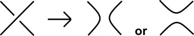
Figure 1. smoothing

In [2] and [14], the following ordering on links is defined.

Definition 1.2.

Let $D_{L_{1}}$ and $D_{L_{2}}$ be alternating link diagrams in $S^{2}$. We say $D_{L_{1}}\subseteq D_{L_{2}}$ if $D_{L_{2}}$ contains $D_{L_{1}}$ as a connected component after smoothing some crossing points of $D_{L_{2}}$.

Let $L_{1}$ and $L_{2}$ be alternating links in $S^{3}$. Then, we say $L_{1}\leq L_{2}$ if for any minimal crossing alternating link diagram $D_{L_{2}}$ of $L_{2}$, there is a minimal crossing alternating link diagram $D_{L_{1}}$ of $L_{1}$ such that $D_{L_{1}}\subseteq D_{L_{2}}$.

These orderings on links and diagrams are called smoothing orders in [2]. Note that smoothing orders become partial orderings. Let us denote the minimal crossing number of $L$ by $c(L)$. If $L_{1}\leq L_{2}$, then $c(L_{1})\leq c(L_{2})$. We can check the well-definedness by using this observation. Actually, if $L_{1}\leq L_{2}$ and $L_{2}\leq L_{1}$, then $c(L_{1})=c(L_{2})$ and there is no smoothed crossing point. So $L_{1}=L_{2}$. Next, if $L_{1}\leq L_{2}$ and $L_{2}\leq L_{3}$, then $L_{1}\leq L_{3}$ by defintion. Note that we can define $\leq$ for any two links by ignoring alternating conditions. But in this paper we consider only alternating links and alternating link diagrams. The Borromean rings $\rm{Brm}$ are an alternating link in $S^{3}$ whose diagram looks as in Figure 2. We fix this diagram and denote it by $\rm{Brm}$ too.

Figure 2. The Borromean rings

Definition 1.3.

$\mathcal{L}_{\overline{\rm{Brm}}}=\{$ an alternating link $L$ in $S^{3}$ such that $\rm{Brm}\nleq L\}$, where $\rm{Brm}$ is the Borromean rings.

Denote $\Sigma(L)$ a double branched covering of $S^{3}$ branched along a link $L$. The following theorem is proved in [16]:

Theorem 1.1.

Let $L$ be a link in $S^{3}$. If $L$ satisfies the following conditions:

• $L\in\mathcal{L}_{\overline{\rm{Brm}}}$,

• $\Sigma(L)$ is a rational homology three-sphere,

then $\Sigma(L)$ is a strong L-space and a graph manifold (or a connected sum of graphmanifolds).

A graph manifold is defined as follows.

Definition 1.4.

A closed oriented three manifold $Y$ is a graph manifold if $Y$ can be decomposed along embedded tori into finitely many Seifert manifolds.

In [16], we also defined the following class of manifolds.

Definition 1.5.

$(T,\sigma,w)$ is an alternatingly weighted tree when the following three conditions hold.

• $T$ is a disjoint union of trees (i.e a disjoint union of simply connected, connected graphs). Let $V(T)$ denote the set of all vertices of $T$.

• $\sigma:V(T)\rightarrow\{\pm 1\}$ is a map such that if two vertices $v_{1}$, $v_{2}$ are connected by an edge, then $\sigma(v_{1})=-\sigma(v_{2})$.

• $w:V(T)\rightarrow\mathbb{Q}_{\geq 0}\cup\{\infty\}$ is a map.

Denote $\mathcal{T}$ the set of all alternatingly weighted trees. For an alternatingly weighted tree $(T,\sigma,w)$, shortly $T$, we define a three manifold $Y_{T}$ as follows. First, we can take a realization of the tree $T$ in $\mathbb{R}^{2}\subset S^{3}$. For each vertex $v$, we introduce the unknot in $S^{3}$. Next if two verteces in $T$ are connected by an edge, we link the corresponding two unknots with linking number $\pm 1$. Thus, we get a link $L_{T}$ in $S^{3}$. Then, we can get a new closed oriented three-manifold $Y_{T}$ by the surgery of $S^{3}$ along every unknot component of $L_{T}$ with the surgery coefficients $\sigma(v)w(v)$ (see Figure 3)

This process gives a natural map $\mathcal{T}\rightarrow\mathcal{M}_{\mathcal{T}}=\{Y_{T};T\in\mathcal{T}\}/\text{homeo}$.

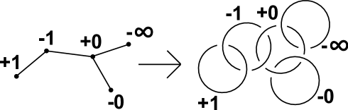
Figure 3.

However, we can prove that these classes are equivalent as follows (see [16]).

Theorem 1.2.

The set of the three manifolds $Y_{T}$ induced from alternatingly weighted trees $(T,\sigma,w)$ is equal to the set of the branched double coverings $\Sigma(L)$ of $S^{3}$ branced along $L$ with $\rm{Brm}\nleq L\}$. That is, $\mathcal{M}_{\mathcal{T}}=\mathcal{L}_{\overline{\rm{Brm}}}$.

Definition 1.6.

A Heegaard diagram is called strong if the induced boundary map of Heegaard Floer chain complex vanishes.

Then, we prove the following classification theorem.

Theorem 1.3.

Let $(\Sigma,\alpha,\beta,z)$ be a strong Heegaard diagram representing a strong $L$-space $Y$. If the genus of $\Sigma$ is at most three, then $Y$ is in $\mathcal{L}_{\overline{\rm{Brm}}}=\mathcal{M}_{\mathcal{T}}$.

2. Heegaard-Floer homology and L-spaces

The Heegaard Floer homology of a closed oriented three manifold $Y$ is defined from a pointed Heegaard diagram representing $Y$. Let $f$ be a self-indexing Morse function on $Y$ with $1$ index zero critical point and $1$ index three critical point. Then, $f$ gives a Heegaard splitting of $Y$. That is, $Y$ is given by glueing two handlebodies $f^{-1}([0,3/2])$ and $f^{-1}([3/2,3])$ along their boundaries. If the number of index one critical points or the number of index two critical points of $f$ is $g$, then $\Sigma=f^{-1}(3/2)$ is a closed oriented genus $g$ surface. We fix a gradient flow on $Y$ corresponding to $f$. We get a collection $\alpha=\{\alpha_{1},\cdots,\alpha_{g}\}$ of $\alpha$ curves on $\Sigma$ which flow down to the index one critical points, and another collection $\beta=\{\beta_{1},\cdots,\beta_{g}\}$ of $\beta$ curves on $\Sigma$ which flow up to the index two critical points. Let $z$ be a point in $\Sigma\setminus(\alpha\cup\beta)$. The tuple $(\Sigma,\alpha,\beta,z)$ is called a pointed Heegaard diagram for $Y$. Note that $\alpha$ and $\beta$ curves are characterized as pairwise disjoint, homologically linearly independent, simple closed curves on $\Sigma$. We can assume $\alpha$-curves intersect $\beta$-curves transversaly.

Next, we review the definition of the Heegaard Floer chain complex.

Let $(\Sigma,\alpha,\beta,z)$ be a pointed Heegaard diagram for $Y$. The $g$-fold symmetric product of the closed oriented surface $\Sigma$ is defined by $\rm{Sym}^{g}(\Sigma)=\Sigma^{\times g}/S_{g}$. That is, the quotient of $\Sigma^{\times g}$ by the natural action of the symmetric group on $g$ letters.

Let us define $\mathbb{T}_{\alpha}=\alpha_{1}\times\cdots\times\alpha_{g}/S_{g}$ and $\mathbb{T}_{\beta}=\beta_{1}\times\cdots\times\beta_{g}/S_{g}$.

Then, the chain complex $\widehat{CF}(\Sigma,\alpha,\beta,z)$ is defined as a free $\mathbb{Z}_{2}$-module generated by the elements of

$$\mathbb{T}_{\alpha}\cap\mathbb{T}_{\beta}=\{x=(x_{1\sigma(1)},x_{2\sigma(2)},\cdots,x_{g\sigma(g)})|x_{i\sigma(i)}\in\alpha_{i}\cap\beta_{\sigma(i)},\sigma\in S_{g}\}.$$

Then, the boundary map $\widehat{\partial}$ is given by

(1) $$\widehat{\partial}x=\sum_{y\in\mathbb{T}_{\alpha}\cap\mathbb{T}_{\beta}}c(x,y)\cdot y,$$

where $c(x,y)\in\mathbb{Z}_{2}$ is defined by counting the number of pseudo-holomorphic Whitney disks. For more details, see [11].

Definition 2.1.

[11] The homology of the chain complex $(\widehat{CF}(\Sigma,\alpha,\beta,z),\widehat{\partial})$ is called the Heegaard Floer homology of a pointed Heegaard diagram. We denote it by $\widehat{HF}(\Sigma,\alpha,\beta,z)$.

Remark.

For appropriate pointed Heegaard diagrams representing $Y$, their Heegaard Floer homologies become isomorphic. So we can define the Heegaard Floer homology of $Y$. Denote it by $\widehat{HF}(Y)$. (For more details, see [11]).

In this paper, we consider only L-spaces, in particular strong L-spaces. The following proposition enables us to define strong L-spaces in another way. The second condition comes from [6].

Proposition 2.1.

Let $(\Sigma,\alpha,\beta,z)$ be a pointed Heegaard diagram representing a rational homology sphere $Y$. Then, the following two conditions (1) and (2) are equivalent.

1. the boundary map $\widehat{\partial}$ is the zero map, and $Y$ is an $L$-apace.

2. $|\mathbb{T}_{\alpha}\cap\mathbb{T}_{\beta}|=|H_{1}(Y;\mathbb{Z})|$.

For example, any lens-spaces are strong L-spaces. Actually, we can draw a genus one Heegaard diagram representing $L(p,q)$ for which the two circles $\alpha$ and $\beta$ meet transversely in $p$ points. That is, $|\mathbb{T}_{\alpha}\cap\mathbb{T}_{\beta}|=|H_{1}(L(p,q);\mathbb{Z})|=p$.

To prove this proposition, we recall that the Heegaard Floer homology $\widehat{HF}(Y)$ admits a relative $\mathbb{Z}/2\mathbb{Z}$ grading([10]) By using this grading, the Euler characteristic satisfies the following equation.

$$\chi(\widehat{HF}(Y,s))=|H_{1}(Y;\mathbb{Z})|.$$

Proof.

The first condition tells us that $\widehat{CF}(Y)$ becomes a $\mathbb{Z}_{2}$-vector space with dimension $|H_{1}(Y;\mathbb{Z})|$. By definition of $\widehat{CF}(Y)$, we get that $|\mathbb{T}_{\alpha}\cap\mathbb{T}_{\beta}|=|H_{1}(Y;\mathbb{Z})|$. Conversely, the second condition and the above equation tell us that both $\widehat{CF}(Y)$ and $\widehat{HF}(Y)$ become $\mathbb{Z}_{2}$-vector spaces with dimension $|H_{1}(Y;\mathbb{Z})|$. Therefore, the first condition follows. ∎

3. Strong diagram and induced matrix

3.1. Characterization of strong diagram

Let $(\Sigma,\alpha,\beta)$ be a Heegaard diagram. Fix orientations of $\alpha$- and $\beta$-curves. Let $\{f_{1},\cdots,f_{g}\}$ be pairwise disjoint simple closed oriented curves with $\#(f_{i}\cap\alpha_{j})=+\delta_{ij}$ (see Figure 4). Then, $\{f_{1},\cdots,f_{g}\}$ generates $H_{1}(Y;\mathbb{Z})$. So $\beta_{j}$ can be written as linear combinations

$$\beta_{j}=\sum^{g}_{i=1}a_{ij}f_{i},\text{ where }a_{ij}\in\mathbb{Z}.$$

In other words, $a_{ij}$ is defined as the algebraic intersection number of $\alpha_{i}$ and $\beta_{j}$, i.e., $a_{ij}=\#(\alpha_{i}\cap\beta_{j})$. Let us define $A=(a_{ij})$.

Figure 4. A generator of $H_{1}(Y;\mathbb{Z})$

Next, let $b_{ij}$ be the number of the elements of the set $\alpha_{i}\cap\beta_{j}$. $b_{ij}$ become non negative integers. Let $B=(b_{ij})$. By the definition of $a_{ij}$ and $b_{ij}$, it is easy to see that $|a_{ij}|\leq b_{ij}$. Moreover, we get that $|\rm{det}(A)|=|H_{1}(Y;\mathbb{Z})|$ and $\overline{\rm{det}}(B)=\mathbb{T}_{\alpha}\cap\mathbb{T}_{\beta}$, where

$$\overline{\rm{det}}(B)=\sum_{\sigma\in S_{g}}b_{1\sigma(1)}\cdots b_{g\sigma(g)}.$$

If $(\Sigma,\alpha,\beta)$ is a strong Heegaard diagram, then $|\rm{det}(A)|=\overline{\rm{det}}(B)$ by its definition. Now we describe a characterization of strong Heegaard diagrams.

Lemma 3.1.

A Heegaard diagram $(\Sigma,\alpha,\beta)$ is strong if and only if $A$ is effective and $|a_{ij}|=b_{ij}$ for all $(i,j)$.

Proof.

Let $(\Sigma,\alpha,\beta)$ be a Heegaard diagram and define $A$ and $B$ as above. Then, $|\rm{det}(A)|$ and $\overline{\rm{det}}(B)$ are expanded as follows.

$$|\rm{det}(A)|=\bigl{|}\sum_{\rm{sgn}(\sigma)=+1}a_{1\sigma(1)}\cdots a_{g\sigma(g)}-\sum_{\rm{sgn}(\sigma)=-1}a_{1\sigma(1)}\cdots a_{g\sigma(g)}\bigr{|},\text{ and }$$

$$\overline{\rm{det}}(B)=\sum_{\rm{sgn}(\sigma)=+1}b_{1\sigma(1)}\cdots b_{g\sigma(g)}+\sum_{\rm{sgn}(\sigma)=-1}b_{1\sigma(1)}\cdots b_{g\sigma(g)}.$$

By using the triangle inequality,

$$\overline{\rm{det}}(A)=\bigl{|}\sum_{\rm{sgn}(\sigma)=+1}a_{1\sigma(1)}\cdots a_{g\sigma(g)}-\sum_{\rm{sgn}(\sigma)=-1}a_{1\sigma(1)}\cdots a_{g\sigma(g)}\bigr{|}$$

$$\leq\sum_{\rm{sgn}(\sigma)=+1}|a_{1\sigma(1)}\cdots a_{g\sigma(g)}|+\sum_{\rm{sgn}(\sigma)=-1}|a_{1\sigma(1)}\cdots a_{g\sigma(g)}|.$$

This inequation becomes the equality if and only if $A$ is effective.

On the other hand, the inequality $|a_{ij}|\leq b_{ij}$ implies that

$$|\rm{det}(B)|=\sum_{\rm{sgn}(\sigma)=+1}b_{1\sigma(1)}\cdots b_{g\sigma(g)}+\sum_{\rm{sgn}(\sigma)=-1}b_{1\sigma(1)}\cdots b_{g\sigma(g)}$$

$$\geq\sum_{\rm{sgn}(\sigma)=+1}|a_{1\sigma(1)}\cdots a_{g\sigma(g)}|+\sum_{\rm{sgn}(\sigma)=-1}|a_{1\sigma(1)}\cdots a_{g\sigma(g)}|.$$

This inequation becomes the equality if and only if $|a_{ij}|=b_{ij}$ for all $(i,j)$.

Thus, this lemma follows.

∎

Definition 3.1.

Let $(\Sigma,\alpha,\beta)$ be a strong Heegaard diagram and orient $\alpha$- and $\beta$- curves. The induced matrix $A_{(\Sigma,\alpha,\beta)}$ is defined by $A_{(\Sigma,\alpha,\beta)}=(\#(\alpha_{i}\cap\beta_{j}))_{ij}$.

3.2. Equivalence class of matrices

Definition 3.2.

Let $A$ be a $g\times g$ effective matrix. $A$ is not maximal if $A$ can be changed into a new effective matrix $A^{\prime}$ by replacing some $0$-component of $A$ with $+1$ or $-1$.

Definition 3.3.

Let $A=(a_{ij})$ and $B=(b_{ij})$ be $g\times g$ matrices. We say $A\sim B$ if $A$ can be changed into a new matrix $A^{\prime}$ so that each $(i,j)$-component of $A^{\prime}$ has the same signature $\{+,-,0\}$ as the $(i,j)$-component of $B$ by some of the following operations.

• to permutate two rows or two columns,

• to multiple a row or a column by $(-1)$,

• to transpose the matrix.

Note that if an effective (or maximal) matrix $A$ is equivalent to $B$, then $B$ is also effective (or maximal). Thus, we can define

$$E_{g}=\{A:\text{ effective }\}/\sim,\text{ and }$$

$$ME_{g}=\{A:\text{ maximal and effective }\}/\sim\subset E_{g}.$$

Definition 3.4.

Let $[A]$ and $[B]$ be two elements of $E_{g}$. We say $[A]\leq[B]$ if we can change $A$ into $A^{\prime}$ by replacing some zero components of $A$ by $+1$ or $-1$ so that the new class $[A^{\prime}]$ is equal to $[B]$.

Note that this ordering tells us that an element of $ME_{g}$ is maximal in $E_{g}$.

For $g=2$, we can prove easily that there exists only one maximal effective matrix $A_{2}$, i.e., $ME_{g}=\{[A_{2}]\}$;

$$A_{2}=\left(\begin{array}[]{@{\,}cccc@{\,}}+&+\\ -&+\end{array}\right),$$

where we consider only signatures of components of matrices.

Lemma 3.2.

For $g=3$, there exists only one maximal effective matrix $A_{3}$, where

$$A_{3}=\left(\begin{array}[]{@{\,}cccc@{\,}}+&+&+\\ -&+&+\\ 0&-&+\end{array}\right),$$

i.e., $ME_{g}=\{[A_{3}]\}$

Proof.

It is easy to see that $A_{3}$ is a maximal effective matrix. Let $A$ be a maximal effective $3\times 3$ matrix. We prove $A\sim A_{3}$. First, put

$$A=\left(\begin{array}[]{@{\,}cccc@{\,}}x_{1}&x_{2}&x_{3}\\ x_{4}&x_{5}&x_{6}\\ x_{7}&x_{8}&x_{9}\end{array}\right).$$

Since $A$ is maximal, we can assume that the diagonal components of $A$ are all positive, i.e., $x_{1}=x_{5}=x_{9}=+$. We can also assume that there exists at least one $0$ component, and we can put $x_{7}=0$ (by permutating rows and columns.) Next, we consider the signature of $x_{4}$.

• If $x_{4}=0$, we can put $x_{6}=+$ and $x_{8}=-$ because $A$ is maximal. (by permutating rows and columns). Then, we can assign arbitrary signatures to $x_{2}$ and $x_{3}$. ($A$ is still effective.) By multipling second or third columns by $(-1)$, we can assume $x_{2}=x_{3}=+$. This operations may change the signature of $x_{5}$, $x_{6}$,$x_{8}$ and $x_{9}$. But by multipling second or third rows by $(-1)$ or permutating rows and columns, we can assume $x_{5}=x_{6}=x_{9}=+$ and $x_{8}=-$. Thus, all signatures of $A$ are decided, however $A$ is not maximal because we can take $x_{4}$ to be positive. This is contradiction.

  $$A\to\left(\begin{array}[]{@{\,}cccc@{\,}}+&x_{2}&x_{3}\\ x_{4}&+&x_{6}\\ 0&x_{8}&+\end{array}\right)\to\left(\begin{array}[]{@{\,}cccc@{\,}}+&x_{2}&x_{3}\\ 0&+&x_{6}\\ 0&x_{8}&+\end{array}\right)\to\left(\begin{array}[]{@{\,}cccc@{\,}}+&x_{2}&x_{3}\\ 0&+&+\\ 0&-&+\end{array}\right)\to\left(\begin{array}[]{@{\,}cccc@{\,}}+&+&+\\ 0&+&+\\ 0&-&+\end{array}\right)$$

  .

• If $x_{4}=+$, by multipling second row and column by $(-1)$, we can change so that $x_{4}=-$.

• If $x_{4}=-$, then $x_{2}=+$ because $A$ is maximal. If $x_{8}=0$, we can transpose $A$ and we return to the case when $x_{4}=0$. So $x_{8}\neq 0$. Moreover, we can put $x_{8}=-$ by multipling third rows and columns by $(-1)$. Lastly, $x_{3}$ and $x_{6}$ must be positive because $A$ is maximal. Thus, $A\sim A_{3}$.

  $$A\to\left(\begin{array}[]{@{\,}cccc@{\,}}+&x_{2}&x_{3}\\ -&+&x_{6}\\ 0&x_{8}&+\end{array}\right)\to\left(\begin{array}[]{@{\,}cccc@{\,}}+&+&x_{3}\\ -&+&x_{6}\\ 0&x_{8}&+\end{array}\right)\to\left(\begin{array}[]{@{\,}cccc@{\,}}+&+&x_{3}\\ -&+&x_{6}\\ 0&-&+\end{array}\right)\to\left(\begin{array}[]{@{\,}cccc@{\,}}+&+&+\\ -&+&+\\ 0&-&+\end{array}\right)=A_{3}$$

  .

∎

Now we define $A^{\prime}_{3}$ as follows.

$$A^{\prime}_{3}=\left(\begin{array}[]{@{\,}cccc@{\,}}+&0&+\\ -&+&0\\ 0&-&+\end{array}\right).$$

Note that $[A^{\prime}_{3}]\leq[A]$.

4. In the case $g=2$

4.1. Types of strong diagrams with $g=2$

First, recall that we can describe a Heegaard diagram $(\Sigma,\alpha,\beta)$ in $\mathbb{R}^{2}$ as in Figure 5, where $2g$ signed oriented circles are $\beta$-curves and oriented arcs are $\alpha$ curves. By attaching the corresponding $\beta$ circles, we recover the Heegaard diagram $(\Sigma,\alpha,\beta)$. Denote each $\beta$-circle by $\beta_{j}^{+}$ or $\beta_{j}^{-}$.

Figure 5. examples of Heegaard diagrams ($g=2,3$)

Each $\alpha$-curve is divided into arcs by $\beta$-circles, and each arc is oriented and has its endpoints at $\beta_{j}^{\pm}$. So let us denote the set of $\alpha_{i}$-arcs from $\beta_{j}^{\pm}$ to $\beta_{j^{\prime}}^{\pm}$ by $\Gamma_{i}(\pm j,\pm j^{\prime})$. We put $\Gamma_{i}(\pm j^{\prime},\pm j)=\Gamma_{i}(\pm j,\pm j^{\prime})$ and $\Gamma(\pm j,\pm j^{\prime})=\Gamma(\pm j^{\prime},\pm j)=\amalg_{i}\Gamma_{i}(\pm j,\pm j^{\prime})$. Moreover, let us denote the union of all elements in $\Gamma(\pm j,\pm j^{\prime})$ by $\Gamma^{\prime}(\pm j,\pm j^{\prime})\subset S^{2}$. For example, the following $\alpha$-arc is an element in $\Gamma_{1}(+1,-2)$.

Figure 6. an element in $\Gamma_{1}(+1,-2)$

Let us consider the $g=2$ case.

Let $(\Sigma,\alpha,\beta)$ be a strong diagram representing $Y$. By Lemma 3.1, the induced matrix $A_{(\Sigma,\alpha,\beta)}$ is effective. Now we first consider the case when $A_{(\Sigma,\alpha,\beta)}$ is $A_{2}$. We call such a diagram an $A_{2}$-strong diagram. There exist just $8$ $\Gamma$-sets which may have some elements as follows.

$$\Gamma_{1}(+\{1,2\},-\{1,2\}),$$

$$\Gamma_{2}(-1,+1),\Gamma_{2}(+2,-2),\Gamma_{2}(+2,+1),\Gamma_{2}(-1,-2),$$

where $\{1,2\}$ means $1$ or $2$.

Now we prepare a notation. Let $E$ a subset of $S^{2}$. For two elements $\gamma_{1}$ and $\gamma_{2}$ in $\Gamma(\pm j,\pm j^{\prime})$, we say $\gamma_{1}\sim\gamma_{2}$ out of $E$ if $\gamma_{1}$ and $\gamma_{2}$ are isotopic on $(S^{2}\setminus E,\beta_{j}^{\pm}\cup\beta_{j^{\prime}}^{\pm})$.

Recall that we can transform a Heegaard diagram by isotopies and handle-slides and stabilizations. For two $\alpha$- or $\beta$-curves, (for example $(\alpha_{1},\alpha_{2})$, ) we can get a new pair of curves by adding one curve to the other curve (for example $(\alpha_{1},\alpha_{2}\pm\alpha_{1})$) (see Figure 7). Denote this handle-slide by $\pm\alpha_{1}\leadsto\alpha_{2}$. In particular, for $\beta$-curves, we denote a handle-slide by $\beta_{j}^{\pm}\leadsto\beta_{j^{\prime}}^{\pm}$.

Figure 7. Handle-slide

Proposition 4.1.

Let $(\Sigma,\alpha,\beta)$ be an $A_{2}$-strong diagram. Then, $(\Sigma,\alpha,\beta)$ can be transformed by handle-slides and isotopies (if it is necessary) so that the new diagram is strong and $\Gamma(+j,-j)$ has at least one element for each $j=1,2$. (However, The new diagram may not be $A_{2}$-strong.)

Proof.

We prove this proposition in two steps.

1. We can transform $(\Sigma,\alpha,\beta)$ so that $\Gamma(+2,-2)\neq\emptyset$.

2. If $\Gamma(+2,-2)\neq\emptyset$, we can transform the diagram so that $\Gamma(+1,-1)\neq\emptyset$ (while keeping the condition $\Gamma(+2,-2)\neq\emptyset$).

In each step, we must take a strong diagram.

Step 1 Let $(\Sigma,\alpha,\beta)$ be an $A_{2}$-strong diagram. If $\Gamma(+2,-2)\neq\emptyset$, there is nothing to do.

Suppose that $\Gamma(+2,-2)=\emptyset$. Since $\#(\alpha_{2}\cap\beta_{2})\neq 0$, we get that $\Gamma(+2,+1)\neq\emptyset$ and $\Gamma(-1,-2)\neq\emptyset$. For any two element $\gamma_{1}$ and $\gamma_{2}$ in $\Gamma(+2,+1)$, we get that $\gamma_{1}\sim\gamma_{2}$ out of $(\beta_{2}^{\mp}\cup\beta_{1}^{\mp}\cup\Gamma^{\prime}(-1,-2))$ because $S^{2}\setminus(\beta_{2}^{\mp}\cup\beta_{1}^{\mp}\cup\Gamma^{\prime}(-1,-2))$ consists of disjoint disks. Then, we can transform the diagram by a handle-slide $\beta_{2}^{+}\leadsto\beta_{1}^{+}$. Note that the new diagram is strong but not $A_{2}$-strong because $\Gamma_{2}(-1,-2)=\emptyset$.

Figure 8.

Step 2 Let $(\Sigma,\alpha,\beta)$ be an $A_{2}$-strong diagram with $\Gamma(+2,-2)\neq\emptyset$. If $\Gamma(+1,-1)\neq\emptyset$, there is nothing to do.

Suppose that $\Gamma(+1,-1)=\emptyset$. Since $\#(\alpha_{2}\cap\beta_{1})\neq 0$, we get that $\Gamma(+2,+1)\neq\emptyset$ and $\Gamma(-1,-2)\neq\emptyset$. For any two element $\gamma_{1}$ and $\gamma_{2}$ in $\Gamma(+2,+1)$, $\gamma_{1}\sim\gamma_{2}$ out of $(\beta_{2}^{\mp}\cup\beta_{1}^{\mp}\cup\Gamma^{\prime}(-1,-2))$, because $S^{2}\setminus(\beta_{2}^{\mp}\cup\beta_{1}^{\mp}\cup\Gamma^{\prime}(-1,-2)\cup\Gamma^{\prime}(+2,-2))$ also consists of disjoint disks. Then, we can transform the diagram by handle-slides $\beta_{1}^{+}\leadsto\beta_{2}^{+}$ finitely many times (see Figure 9). In finitely many steps, we will get an $A_{2}$-strong Heegaard diagram where $\Gamma(+1,-1)\neq\emptyset$. We also get $\Gamma(+2,-2)\neq\emptyset$ because the set $\alpha_{1}\cap\beta_{2}$ becomes non empty after these handle-slides.

Figure 9.

∎

Proposition 4.2.

Let $(\Sigma,\alpha,\beta)$ be an $A_{2}$-strong diagram. Suppose that $\Gamma(+j,-j)\neq\emptyset$ for each $j=1,2$. Then, $(\Sigma,\alpha,\beta)$ is of type (a) or (b) shown in Figure 10.

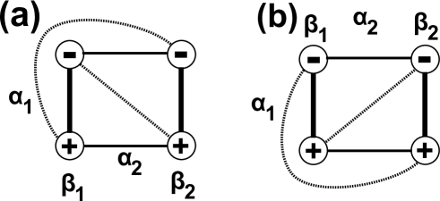
Figure 10. type (a) and type (b)

Proof.

It is easy to see that there are at most two possible types of diagrams under these assumptions. They are type (a) and type (b). ∎

Note that these two types of diagrams are equivalent under permutations of $\alpha$-curves and changes of the orientations of $\beta$-circles. Thus, we consider only the type (a).

4.2. Surgery representations ($g=2$)

In this subsection, we give surgery representations of the diagrams. To do this, we first study about $\Gamma(+j,-j)$ for $j=1,2$ more precisely. After that, we consider auxiliary attaching circles $\gamma=(\gamma_{1},\gamma_{2})$.

Let $(\Sigma,\alpha,\beta)$ be an $A_{2}$-strong diagram of type (a) in Proposition 4.2.

$\Gamma(+1,-1)$:

The neighborhood of $\beta_{1}$-circle looks as in Figure 11.

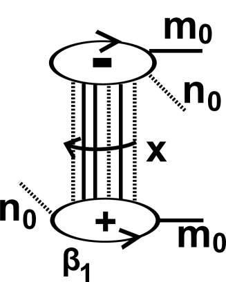
Figure 11.

Let $n_{0}=\#\Gamma(+1,-2)=\#\Gamma(+2,-1)>0$ and $m_{0}=\#\Gamma(+2,+1)=\#\Gamma(-1,-2)>0$. Since $\Gamma(+1,-1)=\Gamma_{1}(+1,-1)\amalg\Gamma_{2}(-1,+1)$, we can define $x=(n_{1},m_{1},n_{2},m_{2},\cdots,n_{k},m_{k})$ to be the sequence of the number of intersection points induced from $\Gamma(+1,-1)$. $n$ comes from $\beta_{1}\cap\alpha_{1}$ and $m$ comes from $\beta_{1}\cap\alpha_{2}$. For example, $x=(n_{1},m_{1},n_{2},m_{2},n_{3})=(1,1,1,2,1)$ for Figure 11. (By the way, this diagram in Figure 11 never become a Heegaard diagram because $m_{1}\neq m_{2}$.)

Since $\beta_{1}^{+}$ and $\beta_{1}^{-}$ are attached to be $\Sigma$, $x$ has the form $(n_{1},m_{1},\cdots,m_{k-1},n_{k})$, $(n_{1}\neq 0,n_{k}\neq 0)$ or $(m_{1},n_{1},\cdots,n_{k-1},m_{k})$, $(m_{1}\neq 0,m_{k}\neq 0)$. Moreover, one of the following two cases happen.

• $x=(n_{1},m_{1},\cdots,m_{k-1},n_{k})$, where $m_{i}=m_{0}$ for all $i$ and $n_{1}=n_{k}$,

• $x=(m_{1},n_{1},\cdots,n_{k-1},m_{k})$, where $n_{i}=n_{0}$ for all $i$ and $m_{1}=m_{k}$.

In each case, take a simple closed oriented curve $\gamma_{1}$ on $\Sigma$ so that the following conditions hold (see Figure 12). If $\Gamma(+1,-1)$ consists of only $\alpha_{1}$-arcs (or only $\alpha_{2}$-arcs), then we take $\gamma_{1}=\beta_{1}$.

• $\gamma_{1}$ intersects each arc in $\Gamma(+2,-1)$ and $\Gamma(-1,-2)$ at a point.

• $\gamma_{1}$ intersects $\beta_{1}$ at some points, but does not intersect $\beta_{2}$.

• If $x=(n_{1},m_{1},\cdots,m_{k-1},n_{k})$, $\gamma_{1}$ intersects only $\alpha_{1}$-arcs in $\Gamma(+1,-1)$.

• If $x=(m_{1},n_{1},\cdots,n_{k-1},m_{k})$, $\gamma_{1}$ intersects only $\alpha_{2}$-arcs in $\Gamma(+1,-1)$.

We consider the new $A_{2}$-strong Heegaard diagram $(\Sigma,\alpha,(\gamma_{1},\beta_{2}))$. Then, the neighborhood of $\gamma_{1}$-circles looks as in Figure 13. (In general, $\beta_{1}$ becomes arcs.) We describe $\beta_{1}$-curve more precisely later.

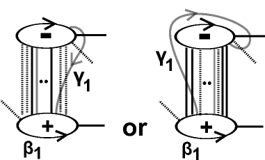
Figure 12. $\gamma_{1}$-curve

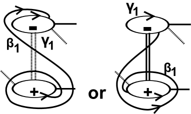
Figure 13. new diagram $(\Sigma,\alpha,(\gamma_{1},\beta_{2}))$

$\Gamma(+2,-2)$:

Next, consider the neighborhood of $\beta_{2}$ as in Figure 14.

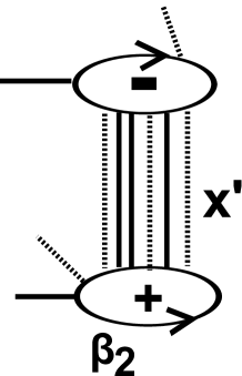
Figure 14.

Similarly, we can define $x^{\prime}$ to be the the sequence of the number of intersection points induced from $\Gamma(+2,-2)$. There exist two cases, where $n^{\prime}$ comes from $\beta_{2}\cap\alpha_{1}$ and $m$ comes from $\beta_{2}\cap\alpha_{2}$.

• $x^{\prime}=(n^{\prime}_{1},m^{\prime}_{1},\cdots,m^{\prime}_{k-1},n^{\prime}_{k})$, where $m^{\prime}_{i}=m^{\prime}_{0}$ for all $i$ and $n^{\prime}_{1}=n^{\prime}_{k}$,

• $x^{\prime}=(m^{\prime}_{1},n^{\prime}_{1},\cdots,n^{\prime}_{k-1},m^{\prime}_{k})$, where $n^{\prime}_{i}=n^{\prime}_{0}$ for all $i$ and $m^{\prime}_{1}=m^{\prime}_{k}$,

In each case, take a simple closed oriented curve $\gamma_{2}$ on $\Sigma$ similarly so that the following conditions hold (see Figure 15). If $\Gamma(+2,-2)$ consists of only $\alpha_{1}$-arcs (or only $\alpha_{2}$-arcs), then we take $\gamma_{2}=\beta_{2}$.

• $\gamma_{2}$ intersects each arc in $\Gamma(+2,-1)$ and $\Gamma(-1,-2)$ at a point.

• $\gamma_{2}$ intersects $\beta_{2}$ at some points, but does not intersect $\beta_{1}$.

• If $x^{\prime}=(n^{\prime}_{1},m^{\prime}_{1},\cdots,m^{\prime}_{k-1},n^{\prime}_{k})$, $\gamma_{2}$ intersects only $\alpha_{1}$-arcs in $\Gamma(+2,-2)$.

• If $x^{\prime}=(m^{\prime}_{1},n^{\prime}_{1},\cdots,n^{\prime}_{k-1},m^{\prime}_{k})$, $\gamma_{2}$ intersects only $\alpha_{2}$-arcs in $\Gamma(+2,-2)$.

We consider the new $A_{2}$-strong Heegaard diagram $(\Sigma,\alpha,\gamma=(\gamma_{1},\gamma_{2}))$. Then, the neighborhood of $\gamma_{2}$-circles looks as in Figure 16. (In general, $\beta_{2}$ becomes arcs.)

We describe $\beta_{2}$-curve more precisely later.

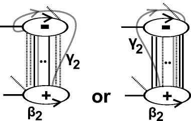
Figure 15. $\gamma_{2}$-curve

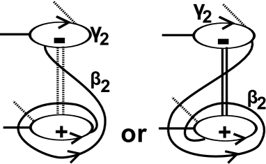
Figure 16. new diagram $(\Sigma,\alpha,\gamma)$

Since the new diagram $(\Sigma,\alpha,\gamma)$ is easier than the old diagram, we classify them into four types (see Figure 17). Actually, the new $\Gamma(+j,-j)$ consists of only $\alpha_{1}$-arcs or $\alpha_{2}$-arcs.

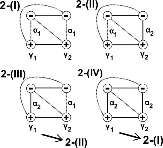
Figure 17. possible types

But, the type 2-(III) (resp. 2-(IV)) are equivalent to the type 2-(II) (resp. 2-(I)) under permutations of $\alpha$-curves and changes of the orientations of $\beta$-curves (before taking $\gamma$-curves).

type 2-(I) In this case, we get that $\#\Gamma(-1,-2)=\#\Gamma(+2,+1)=1$. Thus, we can take another attaching circles $\delta=(\delta_{1},\delta_{2})$ in this diagram such that

• $\#(\delta_{i}\cap\gamma_{j})=\delta_{ij}$ for any $(i,j)$ (thus, $(\Sigma,\delta,\gamma)$ represents $S^{3}$),

• $\delta_{1}$ and $\delta_{2}$ intersects $\alpha_{1}$ and does not intersect $\alpha_{2}$.

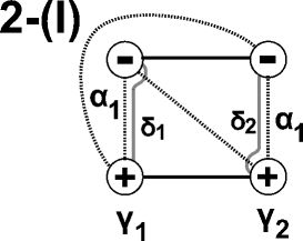
Figure 18. $\delta=(\delta_{1},\delta_{2})$

In this new diagram $(\Sigma,\delta,\gamma)$, $\alpha$ and $\beta$-curves become some framings of some knots in $U_{\delta}\cup U_{\gamma}$. Precisely, we can take three unknots $K_{1}$, $K_{2}$ and $C_{1}$. $K_{1}$ and $K_{2}$ are two unknots in $U_{\gamma}$ whose framings are $\beta$-curves. $C_{1}$ is an unknot in $U_{\delta}$ whose framing is $\alpha_{1}$-curve. Note that $\alpha_{2}$ can be written by $\delta$-curves as a homology in $\Sigma$, so there is no need to consider. These slopes can be determined as follows.

Let $r_{\alpha_{1}}$, $r_{\beta_{1}}$ and $r_{\beta_{2}}$ be the rational numbers representing the surgery framings of $\alpha_{1}$, $\beta_{1}$ and $\beta_{2}$ respectively. Precisely, these rational numbers are determined as follows. Put $r_{\alpha_{1}}=\rm{sgn}(r_{\alpha_{1}})p_{1}/q_{1}$ and $r_{\beta_{i}}=\rm{sgn}(r_{\beta_{i}})p^{\prime}_{i}/q^{\prime}_{i}$ for $i=1,2$. Then,

• $\rm{sgn}(r_{\alpha_{1}})=\rm{sgn}(r_{\beta_{1}})=\rm{sgn}(r_{\beta_{2}})=+1$,

• $p_{1}=\#(\alpha_{1}\cap(\gamma_{1}\cup\gamma_{2})$,

• $q_{1}=\#(\Gamma(+1,-2))$,

• $p^{\prime}_{i}=\#(\beta_{i}\cap\alpha_{2})$, for $i=1,2$.

• $q^{\prime}_{i}=\#(\beta_{i}\cap\gamma_{i})$, for $i=1,2$.

Note that $p_{1}>2q_{1}$ and $p^{\prime}_{i}>q^{\prime}_{i}$ for $i=1,2$. Thus, $|r_{\alpha_{1}}|>2$ and $|r_{\beta_{i}}|>1$ for $i=1,2$. (If $\gamma_{i}=\beta_{i}$, take $r_{\beta_{i}}=\infty$.)

As a result, the three manifold $Y$ obtained from $(\Sigma,\alpha,\beta)$ can be represented as $Y=S^{3}(K_{1},K_{2},C_{1})$ (see Figure 20).

Figure 19.

Figure 20. surgery representation of $Y$

It is easy to see that $Y$ belongs to $\mathcal{M}_{\mathcal{T}}=\mathcal{L}_{\overline{\rm{Brm}}}$. Actually, we can use the following Kirby calculus (see Figure 21 and [4]). If two unknots with the linking number $\pm 1$ have rational framings $+1+r_{1}\geq 1$ and $+1+r_{2}\geq 1$, then we can perform the blow up operation so that the new link has alternating framings. Since $+r_{\beta_{1}}>1$, $+r_{\beta_{2}}>1$ and $+r_{\alpha_{1}}>2$, we get an alternatingly weighted link. Therefore, $Y$ is in $\mathcal{M}_{\mathcal{T}}=\mathcal{L}_{\overline{\rm{Brm}}}$.

Figure 21.

type 2-(II)

In this case, we can take another attaching circles $\delta=(\delta_{1},\delta_{2})$ in this diagram similarly such that

• $\#(\delta_{i}\cap\gamma_{j})=\delta_{ij}$ for any $(i,j)$ (thus, $(\Sigma,\delta,\gamma)$ represents $S^{3}$),

• $\delta_{1}$ intersects $\alpha_{1}$ and does not intersect $\alpha_{2}$.

• $\delta_{2}$ intersects $\alpha_{2}$ and does not intersect $\alpha_{1}$.

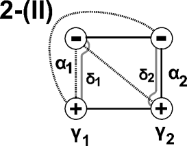
Figure 22. $\delta=(\delta_{1},\delta_{2})$

In this new diagram $(\Sigma,\delta,\gamma)$, we can take four unknots $K_{1}$, $K_{2}$, $C_{1}$ and $C_{2}$. $K_{1}$ and $K_{2}$ are similar in the above case. $C_{1}$ and $C_{2}$ are two unknots in $U_{\delta}$ whose framing is $\alpha_{1}$ and $\alpha_{2}$. These slopes can be determined as follows.

Let $r_{\alpha_{1}}$, $r_{\alpha_{2}}$, $r_{\beta_{1}}$ and $r_{\beta_{2}}$ be the rational numbers representing the surgery framings of $\alpha_{1}$, $\alpha_{2}$, $\beta_{1}$ and $\beta_{2}$ respectively. Precisely, put $r_{\alpha_{i}}=\rm{sgn}(r_{\alpha_{i}})p_{i}/q_{i}$ and $r_{\beta_{i}}=\rm{sgn}(r_{\beta_{i}})p^{\prime}_{i}/q^{\prime}_{i}$ for $i=1,2$. Then,

• $\rm{sgn}(r_{\alpha_{1}})=\rm{sgn}(r_{\beta_{1}})=+1$,

• $\rm{sgn}(r_{\alpha_{2}})=\rm{sgn}(r_{\beta_{2}})=-1$,

• $p_{i}=\#(\alpha_{i}\cap\gamma_{i})$, for $i=1,2$,

• $q_{1}=\#(\Gamma(+1,-2))$,

• $q_{2}=\#(\Gamma(+2,+1))$.

• $p^{\prime}_{1}=\#(\beta_{1}\cap\alpha_{2})/\#(\Gamma(+2,+1))$,

• $p^{\prime}_{2}=\#(\beta_{2}\cap\alpha_{1})/\#(\Gamma(+2,-1))$,

• $q^{\prime}_{i}=\#(\beta_{i}\cap\gamma_{i})$, for $i=1,2$.

Note that $p_{i}>q_{i}$ and $p^{\prime}_{i}>q^{\prime}_{i}$ for $i=1,2$. Thus, $|r_{\alpha_{i}}|>1$ and $|r_{\beta_{i}}|>1$ for $i=1,2$. (If $\gamma_{i}=\beta_{i}$, take $r_{\beta_{i}}=\infty$.)

As a result, the three manifold $Y$ obtained from $(\Sigma,\alpha,\beta)$ can be represented as $Y=S^{3}(K_{1},K_{2},C_{1},C_{2})$ (see Figure 23).

Figure 23. surgery representation of $Y$

It is similar to prove that $Y$ belongs to $\mathcal{M}_{\mathcal{T}}=\mathcal{L}_{\overline{\rm{Brm}}}$.

4.3. Non-maximal cases for $g=2$

In this subsection, we study the case where the induced matrix $A_{(\Sigma,\alpha,\beta)}$ is effective, but not maximal.

Let $(\Sigma,\alpha,\beta)$ be a strong diagram with genus two. If the induced matrix is not $A_{2}$, then

$$A_{(\Sigma,\alpha,\beta)}\sim\left(\begin{array}[]{@{\,}cccc@{\,}}+&0\\ 0&+\end{array}\right)\text{ or }\left(\begin{array}[]{@{\,}cccc@{\,}}+&+\\ 0&+\end{array}\right).$$

The first matrix implies that $Y$ becomes a connected sum of Lens space. If $A_{(\Sigma,\alpha,\beta)}$ is the second matrix, we find that $\Gamma(+2,-2)\neq\emptyset$, $\Gamma(+1,-2)\neq\emptyset$ and $\Gamma(+2,-1)\neq\emptyset$. So the neighborhood of $\beta_{2}$ looks as in Figure 24. Let $x=(n_{1},m_{1},\cdots,m_{k-1},n_{k})$ be the sequence of integers representing $\Gamma(+2,-2)$, where $n$ means $\beta_{2}\cap\alpha_{1}$ and $m$ means $\beta_{2}\cap\alpha_{2}$. Note that $x$ can not be of the form $(m_{1},n_{1},\cdots,n_{k-1},m_{k})$. Since $\Gamma(+2,+1)=\emptyset$, we find that $n_{i}=1$ for all $i$. Thus, we can transform the diagram by handle-slides $\alpha_{1}\leadsto\alpha_{2}$ (see Figure 24).

This new diagram implies that $Y$ is a connected sum of lens spaces.

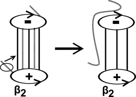
Figure 24. not maximal case

5. Proof of Theorem 1.3

5.1. Types of $A^{\prime}_{3}$-strong diagrams for $g=3$

Let $(\Sigma,\alpha,\beta)$ be a strong diagram representing $Y$ with genus three. Suppose that the equivalence class of the induced matrix satisfies $[A^{\prime}_{3}]\leq[A_{(\Sigma,\alpha,\beta)}]$. We call such a diagram an $A^{\prime}_{3}$-strong diagram. Recall that $[A^{\prime}_{3}]\leq[A_{3}]$. There are just $22$ $\Gamma$-sets which may have some elements as follows.

$$\Gamma_{1}(+\{1,2,3\},-\{1,2,3\}),$$

$$\Gamma_{2}(-1,+1),\Gamma_{2}(+\{2,3\},-\{2,3\}),\Gamma_{2}(+\{2,3\},+1),\Gamma_{2}(-1,-\{2,3\}),$$

$$\Gamma_{3}(-2,+2),\Gamma_{3}(+3,-3),\Gamma_{3}(+3,+2),\Gamma_{3}(-2,-3),$$

where $\{1,2,3\}$ means $1$ or $2$ or $3$.

Proposition 5.1.

Let $(\Sigma,\alpha,\beta)$ be an $A^{\prime}_{3}$-strong diagram. Then, $(\Sigma,\alpha,\beta)$ can be transformed by handle-slides and isotopies (if it is necessary) so that the new diagram is strong and $\Gamma(+j,-j)$ has at least one element for each $j=1,2,3$.

Proof.

We prove this proposition in three steps. Compare this proof with the proof of Proposition 4.1.

1. We can transform the diagram so that $\Gamma(+3,-3)\neq\emptyset$.

2. If $\Gamma(+3,-3)\neq\emptyset$, we can transform the diagram so that $\Gamma(+2,-2)\neq\emptyset$.

3. If $\Gamma(+3,-3)\neq\emptyset$ and $\Gamma(+2,-2)\neq\emptyset$, we can transform the diagram so that $\Gamma(+1,-1)\neq\emptyset$.

In each step, we must take a strong diagram.

Step 1 This step is the same as step 1 of Proposition 4.1. Let $(\Sigma,\alpha,\beta)$ be an $A^{\prime}_{3}$-strong diagram. Suppose $\Gamma(+3,-3)=\emptyset$. Since $\#(\alpha_{3}\cap\beta_{3})\neq 0$, we find that $\Gamma(+3,+2)\neq\emptyset$ and $\Gamma(-2,-3)\neq\emptyset$. Then, we can transform the diagram by a handle-slide $\beta_{3}^{+}\leadsto\beta_{2}^{+}$ similarly.

Figure 25.

Step 2 This step is also the same as step 2 in Proposition 4.1. Let $(\Sigma,\alpha,\beta)$ be an $A^{\prime}_{3}$-strong diagram with $\Gamma(+3,-3)\neq\emptyset$. Suppose that $\Gamma(+2,-2)=\emptyset$. Since $\#(\alpha_{3}\cap\beta_{2})\neq 0$, we get that $\Gamma(+3,+2)\neq\emptyset$ and $\Gamma(-2,-3)\neq\emptyset$. Then, we can transform the diagram by handle-slides $\beta_{2}^{+}\leadsto\beta_{3}^{+}$ finitely many times (see Figure 26). In finitely many steps, we will get an strong Heegaard diagram where $\Gamma(+2,-2)\neq\emptyset$. We also get $\Gamma(+3,-3)\neq\emptyset$ because the set $\alpha_{2}\cap\beta_{3}$ becomes non empty after these handle-slides.

Figure 26.

Step 3 Let $(\Sigma,\alpha,\beta)$ be an $A^{\prime}_{3}$-strong diagram with $\Gamma(+3,-3)\neq\emptyset$, $\Gamma(+2,-2)\neq\emptyset$. Suppose that $\Gamma(+1,-1)=\emptyset$. Since $\#(\alpha_{3}\cap\beta_{2})\neq 0$ by the assumption, we can get Figure 27. Moreover, any two arcs in $\Gamma(+3,-3)$, $\Gamma(+3,+2)$, $\Gamma(-3,-2)$ and $\Gamma(+2,-2)$ are isotopic to each edge of the rectangle respectively. Since $\alpha_{1}\cap\beta_{1}\neq\emptyset$ and $\alpha_{2}\cap\beta_{1}\neq\emptyset$, we get that $\beta_{1}^{+}$ and $\beta_{1}^{-}$ are in or out of the rectangle. Actually, if $\beta_{1}^{+}$ is between two arcs in $\Gamma(-3,-2)$, we find that $\alpha_{1}$ can not intersect $\beta_{1}$. Moreover, if $\beta_{1}^{+}$ is between two arcs in $\Gamma(+3,-3)$, we can transform the diagram by handle-slides $\beta_{1}^{+}\leadsto\beta_{3}^{-}$ finitely many times so that $\beta_{1}^{+}$ is in or out of the rectangle (see Figure 28).

Figure 27. $\Gamma(+3,-3)$, $\Gamma(+3,+2)$, $\Gamma(-3,-2)$ and $\Gamma(+2,-2)$ make a rectangle

Figure 28. positions of $\beta_{1}^{+}$

Assume $\beta_{1}^{+}$ is in the rectangle. There are four possible cases.

• If $\Gamma(+1,-2)\neq\emptyset$, $\Gamma(+1,-3)\neq\emptyset$, $\Gamma(+1,+2)\neq\emptyset$, $\Gamma(+1,+3)\neq\emptyset$ and $\Gamma(+3,-2)\neq\emptyset$, then $\beta_{1}^{-}$ is in one of the three domains adjacent to $\beta_{3}^{-}$. But one of them is impossible because $\Gamma(+2,-1)\neq\emptyset$ (see Figure 29). In the other two cases, we can transform the diagram by handle-slides $\beta_{1}^{-}\leadsto\beta_{3}^{-}$ finitely many times. Thus, we get $\Gamma(+1,-1)\neq\emptyset$. Of course, the diagram is strong and $\Gamma(+3,-3)\neq\emptyset$ and $\Gamma(+2,-2)\neq\emptyset$.

  
  

  Figure 29.

• If $\Gamma(+1,-2)\neq\emptyset$, $\Gamma(+1,-3)\neq\emptyset$, $\Gamma(+1,+2)\neq\emptyset$, $\Gamma(+1,+3)\neq\emptyset$ and $\Gamma(-3,+2)\neq\emptyset$, we can get $\Gamma(+1,-1)\neq\emptyset$ similarly.

• If $\Gamma(+1,-2)\neq\emptyset$, $\Gamma(+1,-3)\neq\emptyset$, $\Gamma(+1,+2)\neq\emptyset$, $\Gamma(+1,+3)\neq\emptyset$, $\Gamma(+3,-2)=\emptyset$ and $\Gamma(-3,+2)=\emptyset$, then $\beta_{1}^{-}$ is in one of the following two domains as in Figure 30 because $\#(\alpha_{1}\cap\beta_{3}^{+})=\#(\alpha_{1}\cap\beta_{3}^{-})$. Thus, we can also transform the diagram by handle-slides $\beta_{1}^{-}\leadsto\beta_{3}^{-}$ finitely many times so that we get $\Gamma(+1,-1)\neq\emptyset$.

  
  

  Figure 30.

• If one of $\Gamma(+1,-2)$, $\Gamma(+1,-3)$, $\Gamma(+1,+2)$, $\Gamma(+1,+3)$ is the empty set, then we can transform the diagram by handle-slides finitely many times so that we get $\Gamma(+1,-1)\neq\emptyset$ as follows.

  • $\Gamma(+1,+3)=\emptyset\Rightarrow\beta_{1}^{+}\leadsto\beta_{2}^{+}$.

  • $\Gamma(+1,-3)=\emptyset\Rightarrow\beta_{1}^{+}\leadsto\beta_{2}^{-}$.

  • $\Gamma(+1,+2)=\emptyset\Rightarrow\beta_{1}^{+}\leadsto\beta_{3}^{+}$.

  • $\Gamma(+1,-2)=\emptyset\Rightarrow\beta_{1}^{+}\leadsto\beta_{3}^{-}$.

∎

Proposition 5.2.

Let $(\Sigma,\alpha,\beta)$ be an $A^{\prime}_{3}$-strong diagram. Suppose $\Gamma(+j,-j)\neq\emptyset$ for $j=1,2,3$. Then, $(\Sigma,\alpha,\beta)$ can be transformed by handle-slides, isotopies, permutations of curves, changes of orientations(if it is necessary) so that the new strong diagram is of one of the following three types 3-(a), 3-(b) and 3-(c) (see Figure 31).

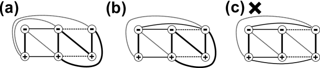
Figure 31. three possoble types

Proof.

By Proposition 5.1, we can assume $\Gamma(+j,-j)\neq\emptyset$ for all $j$. We put $\beta_{1}$ and $\beta_{2}$ as in Figure . Then, $\beta_{3}$ is in one of the three domains as in Figure .

Figure 32. three positions

• The position (i) is impossible because $\Gamma(+3,+2)\neq\emptyset$.

• If $\beta_{3}$ is in (ii), $\beta_{1}$ and $\beta_{2}$ looks as in Figure 33. Since $\Gamma(+1,-2)\neq\emptyset$ and $\Gamma(-1,-2)\neq\emptyset$, we can transform the diagram by handle-slides $(\beta_{1}^{+}\text{ and }\beta_{1}^{-})\leadsto\beta_{2}^{-}$ finitely many times so that the new diagram is also $A^{\prime}_{3}$-strong and $\beta_{3}$ is in the position (iii).

  
  

  Figure 33.

• If $\beta_{3}$ is in (iii), there exist at most two isotopy classes of arcs in $\Gamma(+3,-3)$ (see 34). If there exist two arcs which are not isotopic, then we can transform the diagram by handle-slides $(\beta_{2}^{+}\text{ and }\beta_{2}^{-})\leadsto\beta_{3}^{-}$ finitely many times so that all arcs in $\Gamma(+j,-j)$ are isotopic (see Figure 34).

  
  

  Figure 34.

Since $\Gamma(+3,+2)\neq\emptyset$ and $\Gamma(-3,-2)\neq\emptyset$, we get two possible cases as in Figure 35. But they are equivalent under permutating $\beta_{2}$ and $\beta_{3}$ and reversing the orientation of $\alpha_{3}$.

Figure 35.

Now we can describe all possible cases. There are another $9$ cases, but we can transform these diagrams into one of the three types. ∎

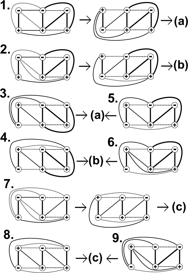
Figure 36.

However, note that the type (c) never happens. Actually, the pattern of the intersection points at $\beta_{3}^{+}$ and $\beta_{3}^{-}$ never coincide, so we can not attach $\beta_{3}$-circles.

5.2. Surgery representations for $g=3$, $\beta$-curves

Let $(\Sigma,\alpha,\beta)$ be an $A^{\prime}_{3}$-strong diagram of type 3-(a) or 3-(b).

$\Gamma(+1,-1)$:

We first consider the neighborhood of $\beta_{1}$. Let $n_{0}=\#\Gamma(+1,-2)+\#\Gamma(+1,-3)$ and $m_{0}=\#\Gamma(+1,+2)+\#\Gamma(+1,+3)$. Then, the argument is the same as in the case when $g=2$.

That is, we can define $x$ to be the sequence of the number of intersection points induced from $\Gamma(+1,-1)$ and one of the following two cases may happen, where $n$ comes from $\beta_{1}\cap\alpha_{1}$ and $m$ comes from $\beta_{1}\cap\alpha_{2}$.

• $x=(n_{1},m_{1},\cdots,m_{k-1},n_{k})$ where $m_{i}=m_{0}$ for all $i$ and $n_{1}=n_{k}$,

• $x=(m_{1},n_{1},\cdots,n_{k-1},m_{k})$ where $n_{i}=n_{0}$ for all $i$ and $m_{1}=m_{k}$.

In each case, take a simple closed oriented curve $\gamma_{1}$ on $\Sigma$ so that the following conditions hold. If $\Gamma(+1,-1)$ consists of only $\alpha_{1}$-arcs (or only $\alpha_{2}$-arcs), then we take $\gamma_{1}=\beta_{1}$.

• $\gamma_{1}$ intersects each arc in $\Gamma(+2,-1)$, $\Gamma(-1,-2)$ and $\Gamma(-1,-3)$ at a point.

• $\gamma_{1}$ intersects $\beta_{1}$ at some points, but does not intersect $\beta_{2}$ and $\beta_{3}$.

• If $x=(n_{1},m_{1},\cdots,m_{k-1},n_{k})$, $\gamma_{1}$ intersects only $\alpha_{1}$-arcs in $\Gamma(+1,-1)$.

• If $x=(m_{1},n_{1},\cdots,n_{k-1},m_{k})$, $\gamma_{1}$ intersects only $\alpha_{2}$-arcs in $\Gamma(+1,-1)$.

We consider the new $A^{\prime}_{3}$-strong Heegaard diagram $(\Sigma,\alpha,(\gamma_{1},\beta_{2},\beta_{3}))$. We describe $\beta_{1}$-curve more precisely later.

$\Gamma(+2,-2)$:

Next, we consider the neighborhood of $\beta_{2}$-circles. The neighborhood of $\beta_{2}$-circles looks as in Figure 37. Then, we can take $\gamma_{2}$ as follows (see Figure 37). If there exists no $\alpha_{3}$-arc in $\Gamma(+2,-2)$, then we need not to take $\gamma_{2}$.

• $\gamma_{2}$ intersects each arc in $\Gamma(-2,-3)$, $\Gamma(+1,-2)$ and $\Gamma(-1,-2)$ at a point.

• $\gamma_{1}$ intersects $\beta_{2}$ at some points, but does not intersect $\beta_{1}$ and $\beta_{3}$.

• $\gamma_{1}$ does not intersect $\alpha_{3}$-arcs in $\Gamma(+2,-2)$.

We consider the new $A^{\prime}_{3}$-strong Heegaard diagram $(\Sigma,\alpha,(\gamma_{1},\gamma_{2},\beta_{3}))$. Then, the neighborhood of $\gamma_{2}$-circles looks as in Figure 37. We describe $\beta_{2}$-curve more precisely later.

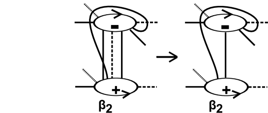
Figure 37. $\gamma_{2}$-curve and new diagram $(\Sigma,\alpha,(\gamma_{1},\gamma_{2},\beta_{3}))$

$\Gamma(+3,-3)$: Lastly, consider the neighborhood of $\beta_{3}$ looks as in Figure 38.

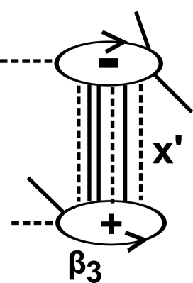
Figure 38.

Similarly, we can define $x^{\prime}$ to be the the sequence of the number of intersection points induced from $\Gamma(+3,-3)$. In this case, it is convinient not to distinguish $\alpha_{1}$ and $\alpha_{3}$. That is, there exist two cases, where $n^{\prime}$ comes from $\beta_{3}\cap\alpha_{3}$ and $m$ comes from $\beta_{3}\cap(\alpha_{1}\cup\alpha_{2})$.

• $x^{\prime}=(n^{\prime}_{1},m^{\prime}_{1},\cdots,m^{\prime}_{k-1},n^{\prime}_{k})$ where $m^{\prime}_{i}=m^{\prime}_{0}$ for all $i$ and $n^{\prime}_{1}=n^{\prime}_{k}$,

• $x^{\prime}=(m^{\prime}_{1},n^{\prime}_{1},\cdots,n^{\prime}_{k-1},m^{\prime}_{k})$ where $n^{\prime}_{i}=n^{\prime}_{0}$ for all $i$ and $m^{\prime}_{1}=m^{\prime}_{k}$.

Moreover, if $x^{\prime}=(m^{\prime}_{1},n^{\prime}_{1},\cdots,n^{\prime}_{k-1},m^{\prime}_{k})$, we find that $n^{\prime}_{i}=1$ for all $i$. Otherwise, $\alpha_{3}$-arcs can not be a closed curve. Then, We can transform the diagram by $m^{\prime}_{1}$ handle-slides $+(\alpha_{1}\text{ and }\alpha_{2})\leadsto\alpha_{3}$ (see Figure 39) so that the new diagram is also $A^{\prime}_{3}$-strong diagram and $\Gamma_{i}(+3,-3)=\emptyset$ for $i=1,2$. As a result, we return to the first case.

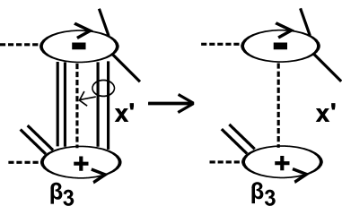
Figure 39.

If $x^{\prime}=(n^{\prime}_{1},m^{\prime}_{1},\cdots,m^{\prime}_{k-1},n^{\prime}_{k})$, take a simple closed oriented curve $\gamma_{3}$ on $\Sigma$ similarly so that the following conditions hold (see Figure 40). If $\Gamma(+3,-3)$ consists of only $\alpha_{3}$-arcs, then we take $\gamma_{3}=\beta_{3}$.

• $\gamma_{3}$ intersects each arc in $\Gamma(-2,-3)$, $\Gamma(+1,-3)$ and $\Gamma(+2,-3)$at a point.

• $\gamma_{3}$ intersects $\beta_{3}$ at some points, but does not intersect $\beta_{1}$ and $\beta_{2}$.

• $\gamma_{3}$ intersects only $\alpha_{3}$-arcs in $\Gamma(+2,-2)$.

We consider the new $A^{\prime}_{3}$-strong Heegaard diagram $(\Sigma,\alpha,\gamma=(\gamma_{1},\gamma_{2},\gamma_{3}))$. Then, the neighborhood of $\gamma_{2}$-circles looks as in Figure 40. (In general, $\beta_{2}$ becomes arcs.) We describe $\beta_{3}$-curve more precisely later.

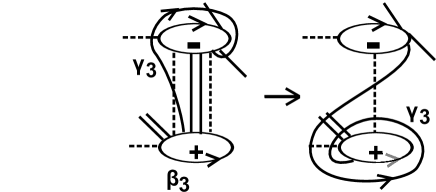
Figure 40. $\gamma_{3}$ and new diagram $(\Sigma,\alpha,\gamma)$

Thus, there exist four possible types (see Figure 41).

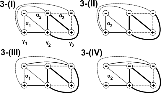
Figure 41. possible four types

In each case, $\beta_{j}$-curves become some surgery framings of some unknots $K_{1}$, $K_{2}$ and $K_{3}$ by attaching $\gamma_{j}$-circles (see Figure 42).

Figure 42.

5.3. Surgery representations for $g=3$, $\alpha$-curves

Now, we recall positive (or negative) Dehn twists.

Definition 5.1.

Let $\Sigma$ be a closed oriented genus $g$ surface and Let $c_{1}$ be a simple closed curve on $\Sigma$. Then, a positive (or negative) Dehn twist is the self-homeomorphism $\pm f(c_{1})$ on $\Sigma$ defined as in Figure 43-(p) and (n) on a neighborhood of $c_{1}$, where a curve $c_{2}$ is mapped to $f(c_{2})$ by $f$. On the other hand, $\pm f(c_{1})$ is identity on $\Sigma\setminus nbd(c_{1})$.

Figure 43. positive/negative Dehm surgery

Let $(\Sigma,\alpha,\beta)$ be an $A^{\prime}_{3}$-strong diagram of type 3-(I), 3-(II), 3-(III) or 3-(IV). Let $c$ be a simple closed curve on $\Sigma$ which intersects $\Gamma(+2,+3)$, $\Gamma(+3,-2)$, $\gamma_{2}$ and $\gamma_{3}$ as in Figure 44. We perform a positive Dehn twist along $c$. Then, $\alpha$-arcs are changed as in Figure 45. Note that $\gamma_{3}$ intersects only $\alpha_{3}$. Thus, $\alpha_{3}$-curves become a surgery framing of a unknot $C_{3}$ in $U_{\alpha}$. We describe the slope precisely later. Let $\alpha^{\prime}_{3}$ be the simple closed curve which intersects only $\gamma_{3}$ at one point (see Figure 46).

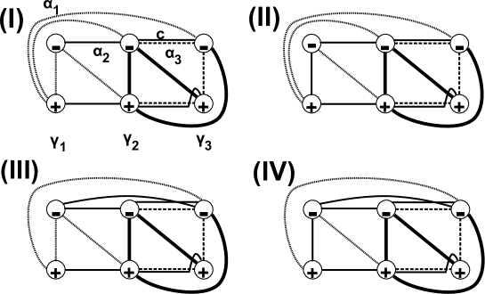
Figure 44.

Figure 45.

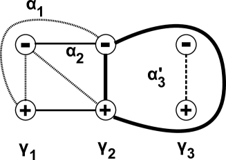
Figure 46.

Next, we consider the simple closed curve $c$ as above again. We perform a negative Dehn twist along $c$ (see Figure 44). Since $\alpha^{\prime}_{3}$ still intersects $\gamma_{3}$ at only one point, we can transform the diagram by a handle-slide $(\Gamma(+1,-3)\text{ and }\Gamma(+2,-3))\leadsto\alpha_{3}$, where $(\Gamma(+1,-3)\leadsto\alpha_{3}$ means the collection of the handle slides $\gamma\leadsto\alpha_{3}$ and $\gamma\in\Gamma(+1,-3)$ (see Figure 47). These operations correspond to the following link (see Figure 48).

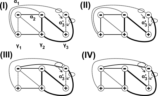
Figure 47.

Figure 48.

The Figure 49 implies that type 3-(I) and 3-(III) induces the same diagrams, and type 3-(II) and 3-(IV) induces the same diagrams. We call these diagrams 3-(I),(III) and 3-(II),(IV). Let us consider the attaching circles $\alpha^{\prime}=(\alpha_{1},\alpha_{2},\alpha^{\prime}_{3})$ and $(\gamma_{1},\gamma_{2},\gamma_{3})$ in Figure 49.

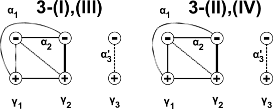
Figure 49.

Define another attaching circles $(\delta_{1},\delta_{2},\delta_{3})$ in each diagram which satisfy the following conditions.

• $\#(\delta_{i}\cap\gamma_{j})=\delta_{ij}$ for any $(i,j)$ (thus, $(\Sigma,\delta,\gamma)$ represents $S^{3}$),

• If in the case of 3-(I),(III), $\delta_{1}$ intersects $\alpha_{1}$ and does not intersect $\alpha_{2}$.

• If in the case of 3-(II),(IV), $\delta_{1}$ intersects $\alpha_{2}$ and does not intersect $\alpha_{1}$.

• $\delta_{2}$ intersects $\alpha$-curves at $N$ points, where $N<\#(\Gamma(+2,-2))+\#(\Gamma(+2,-1))+\#(\Gamma(+2,+1))$.

• $\delta_{3}=\alpha^{\prime}_{3}$

Let us denote $D_{1}$ and $D_{3}$ be properly embedded disks in $U_{\delta}$ such that $\partial{D_{1}}=\delta_{1}$ and $\partial{D_{3}}=\delta_{3}$. If we cut the handlebody $U_{\delta}$ along $D_{1}$ and $D_{3}$, then $U_{\delta}\setminus(D_{1}\cup D_{3})$ becomes a solid torus. Let us denote the core of the solid torus by $C_{2}$. Then,

• $\alpha_{2}$ becomes the surgery framing of $C_{2}$ in the case of 3-(I),(III), and

• $\alpha_{1}$ becomes the surgery framing of $C_{2}$ in the case of 3-(II),(IV).

On the other hand, it is easy to see that there exists a $C_{1}$ in $U_{\delta}$ such that

• $\alpha_{1}$ become the surgery framings of $C_{1}$ in the case of 3-(I),(III), and

• $\alpha_{2}$ become the surgery framings of $C_{1}$ in the case of 3-(II),(IV).

Note that $C_{1}$ becomes a torus knot in $S^{3}$ in genaral. We describe these slopes later.

As a result, a Heegaard diagrams of each type is represented by a surgery of $S^{3}$ along some link (see Figure 50 and 51). Let us denote the framed link induced from 3-(I),(III) by $L(13)$ and the framed link induced from 3-(II),(IV) by $L(24)$. Moreover, let us denote the manifolds induced from these links $L(13)$ and $L(24)$ by $M(13)$ and $M(24)$. Now we denote the framing of these links shortly. Let $r_{\alpha_{i}}$ be the framing of $C_{j}$ corresponding to $\alpha_{i}$ for any $(i,j)$. Let $r_{\beta_{j}}$ be the framing of $K_{j}$ corresponding to $\beta_{j}$ for any $j$.

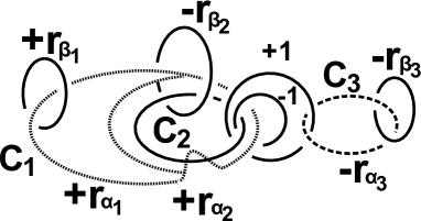
Figure 50. 3-(I),(III)

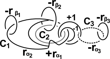
Figure 51. 3-(II),(IV)

5.4. Determination of manifolds for $g=3$

In this subsection, we finish to prove Theorem 1.3. Recall there are two cases to be considered.

3-(I),(III) Let $(\Sigma,\alpha,\beta)$ be an $A^{\prime}_{3}$-strong diagram of type 3-(I),(III) (see Figure 49). Recall that $r_{\alpha_{i}}$ is the framing of $C_{i}$ corresponding to $\alpha_{i}$ for any $i$, and $r_{\beta_{j}}$ is the framing of $K_{j}$ corresponding to $\beta_{j}$ for any $j$.

First, we write these slopes concretely.

• $r_{\alpha_{1}}=+p_{1}/q_{1}+p_{2}+q_{2}-1$, where

  • $p_{1}=\#(\alpha_{1}\cap\gamma_{1})$,

  • $q_{1}=\#\Gamma(+1,-2)$,

  • $p_{2}=\#(\alpha_{1}\cap\gamma_{2})/q_{1}$.

  • $q_{2}=\#(\alpha_{1}\cap\delta_{2})$.

• $r_{\alpha_{2}}=+p^{\prime}_{2}/q^{\prime}_{2}$, where

  • $p^{\prime}_{2}=\#(\alpha_{2}\cap\gamma_{2})$,

  • $q^{\prime}_{2}=\#(\alpha_{2}\cap\delta_{2})$.

• $r_{\alpha_{3}}=-p_{3}/q_{3}$, where

  • $p_{3}=\#(\alpha_{3}\cap\gamma_{3})$,

  • $q_{3}=\#(\alpha_{3}\cap\delta_{3})$.

• $r_{\beta_{1}}=+\#(\beta_{1}\cap\delta_{1})/\#(\beta_{1}\cap\gamma_{1})$.

• $r_{\beta_{2}}=-\#(\beta_{2}\cap\delta_{2})/\#(\beta_{1}\cap\gamma_{1})$.

• $r_{\beta_{3}}=-\#(\beta_{3}\cap\delta_{3})/\#(\beta_{1}\cap\gamma_{1})$.

Then, $C_{1}$ becomes the $(p_{2},q_{2})$-torus knot and it is linking with $C_{2}$, where the framing of the $(p_{2},q_{2})$-torus becomes the integer $p_{2}+q_{2}-1$. We also find that, by easy obsevations,

• $+p_{1}/q_{1}>+1$,

• $r_{\alpha_{2}}>+1$,

• $r_{\beta_{1}}>+1$,

• $r_{\beta_{2}}<-1$,

• $r_{\beta_{3}}<-1$.

Next, we describe the relation between $p_{2}/q_{2}$ and $p^{\prime}_{2}/q^{\prime}_{2}$ precisely. We can represent $p_{2}/q_{2}$ as the continuous fraction expansion as follows.

(2) $$\frac{p_{2}}{q_{2}}=k_{1}+\cfrac{1}{k_{2}+\cfrac{1}{\cdots+\cfrac{1}{k_{n-1}+\cfrac{1}{k_{n}}}}},\text{ where }k_{i}\geq 1\text{ and }k_{n}\geq 2.$$

By using these integers, we put a new rational number $R(p_{2},q_{2},p^{\prime}_{2},q^{\prime}_{2})$ as follows.

(3) $$R(p_{2},q_{2},p^{\prime}_{2},q^{\prime}_{2})=-(k_{n}+\cfrac{1}{k_{n-1}+\cfrac{1}{\cdots+\cfrac{1}{k_{2}+\cfrac{1}{k_{1}-\cfrac{p^{\prime}_{2}}{q^{\prime}_{2}}}}}}).$$

Then, we can prove the following claim.

Claim 5.1.

Let $p_{2}/q_{2}$, $p^{\prime}_{2}/q^{\prime}_{2})$ and $R(p_{2},q_{2},p^{\prime}_{2},q^{\prime}_{2})$ be the rational numbers defined as above. Then, we get that

• $R(p_{2},q_{2},p^{\prime}_{2},q^{\prime}_{2})>0$ if $n$ is odd, and

• $-1<R(p_{2},q_{2},p^{\prime}_{2},q^{\prime}_{2})<0$ if $n$ is even.

Proof.

Originaly, these two rational numbers $p_{2}/q_{2}$ and $p^{\prime}_{2}/q^{\prime}_{2})$ come from the slopes of $\alpha_{1}$ and $\alpha_{2}$ near $\gamma_{2}$. Thus, we study about the neighborhood of $\beta_{2}$ more precisely.

Recall the neighborhood of $\gamma_{2}$ looks as in Figure 52, where we can define $x=(m_{1},n_{1},m_{2},\cdots,n_{\tilde{k}-1},m_{\tilde{k}})$ as the sequence of the number of intersection points induced from $\Gamma(+2,-2)$. $n$ comes from $\gamma_{2}\cap\alpha_{1}$ and $m$ comes from $\gamma_{2}\cap\alpha_{2}$.

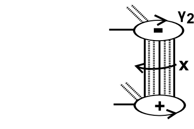
Figure 52.

Note that it is enough to consider the case when $m_{1}=m_{\tilde{k}}$ is not zero. Otherwise, $\#\Gamma(+2,+1)=1$ and we can change the diagram by handle-slides so that $n_{1}=n_{\tilde{k}-1}$ is equal to zero in the new diagram (see Figure 39).

We put $d_{1}=\#\Gamma(+2,+1)$ and $d_{2}=m_{1}=m_{\tilde{k}}$. Moreover, let $1\leq\bar{p}_{2}\leq p_{2}$ and $1\leq\bar{q}_{2}\leq q_{2}$ be positive coprime integers so that $\bar{p}_{2}q_{2}=\bar{q}_{2}p_{2}+1$.

Then, $p^{\prime}_{2}/q^{\prime}_{2}$ can be written by these integers as follows.

$$p^{\prime}_{2}/q^{\prime}_{2}=\frac{\bar{p}_{2}(d_{1}+d_{2})+(p_{2}-\bar{p}_{2})d_{2}}{\bar{q}_{2}(d_{1}+d_{2})+(q_{2}-\bar{q}_{2})d_{2}}=\frac{\bar{p}_{2}+p_{2}z}{\bar{q}_{2}+q_{2}z},\text{ where }z=d_{2}/d_{1}.$$

Actually, $\bar{p}_{2}$ represents the number of the integer $d_{1}+d_{2}$ among the sequence $(m_{1},m_{2},\cdots,m_{\tilde{k}})$ and $\bar{q}_{2}$ represents the number of the integer $d_{1}+d_{2}$ among the sequence $(m_{1},m_{2},\cdots,m_{q_{2}})$. It is easy to see that these integers satisfies $\bar{p}_{2}q_{2}=\bar{q}_{2}p_{2}+1$. Then, we find that $p^{\prime}_{2}/q^{\prime}_{2}$ is written as above.

Since $0<z<+\infty$ we get that $p_{2}/q_{2}<p^{\prime}_{2}/q^{\prime}_{2}<\bar{p}_{2}/\bar{q}_{2}$.

Moreover, we can prove that $\bar{p}_{2}/\bar{q}_{2}$ can be written precisely as follows.

$$\bar{p}_{2}/\bar{q}_{2}=k_{1}+\cfrac{1}{k_{2}+\cfrac{1}{\cdots+\cfrac{1}{k_{n-1}}}},\text{ if }n\text{ is odd.}$$

$$\bar{p}_{2}/\bar{q}_{2}=k_{1}+\cfrac{1}{k_{2}+\cfrac{1}{\cdots+\cfrac{1}{k_{n}-1}}},\text{ if }n\text{ is even.}$$

This equation comes from the Euclidean algorithm. Thus, we also find that the length of the continuous fraction expansion of $p^{\prime}_{2}/q^{\prime}_{2}$ is $n$ or grater than $n$. In particular, $R(p_{2},q_{2},p^{\prime}_{2},q^{\prime}_{2})$ is well-defined.

Finally, we conclude that

$$R(p_{2},q_{2},p^{\prime}_{2},q^{\prime}_{2})=-(k_{n}+\cfrac{1}{k_{n-1}+\cfrac{1}{\cdots+\cfrac{1}{k_{2}+\cfrac{1}{k_{1}-p^{\prime}_{2}/q^{\prime}_{2}}}}})>0,$$

if $n$ is odd, and

$$0>R(p_{2},q_{2},p^{\prime}_{2},q^{\prime}_{2})>-(k_{n}+\cfrac{1}{k_{n-1}+\cfrac{1}{\cdots+\cfrac{1}{k_{2}+\cfrac{1}{k_{1}-\bar{p}_{2}/\bar{q}_{2}}}}})=-1,$$

if $n$ is even. ∎

We consider the framed link $L(13)$ again. Our goal is to prove that $M(13)$ is in $\mathcal{L}_{\overline{\rm{Brm}}}$.

We perform the blow up operations finitely many times so that the new framed link consists of only unknots. First, add $k_{1}$ unknots with framing $-1$ near $C_{2}$ and $C_{1}$ as in Figure 53. After that, the slopes of $C_{1}$ and $C_{2}$ are changed as follows. Denote the new slopes by $r^{1}_{\alpha_{1}}$ and $r^{1}_{\alpha_{2}}$.

• $r_{\alpha_{1}}\leadsto r^{1}_{\alpha_{1}}=r_{\alpha_{1}}-k_{1}q^{0}_{2}$, where $q^{0}_{2}=q_{2}$,

• $r_{\alpha_{2}}\leadsto r^{1}_{\alpha_{2}}=r_{\alpha_{2}}-k_{1}$,

• the new knot $C^{1}_{1}$ induced from $C_{1}$ is linking with $C_{2}$ with the slope $p^{1}_{2}/q^{1}_{2}$, where $p^{1}_{2}$ and $q^{1}_{2}$ are positive coprime integer such that $p_{2}/q_{2}=k_{1}+p^{1}_{2}/q^{1}_{2}$.

Figure 53.

This new link can be transformed into the following link (see Figure 54).

Figure 54.

Next, add $k_{2}$ unknots with framing $-1$ isotopic to $C_{2}$ as in Figure 55. After some Kirby calculus, the slopes of $C_{1}$ and $C_{2}$ are changed as follows.

• $r^{1}_{\alpha_{1}}\leadsto r^{2}_{\alpha_{1}}=r^{1}_{\alpha_{1}}-k_{2}p^{1}_{2}$,

• $r^{1}_{\alpha_{2}}\leadsto r^{2}_{\alpha_{2}}=-\cfrac{1}{k_{2}+\cfrac{1}{-r^{1}_{\alpha_{2}}}}$,

• the new $C^{2}_{1}$ is linking with $C_{2}$ with the slope $p^{2}_{2}/q^{2}_{2}$, where $p^{2}_{2}$ and $q^{2}_{2}$ are positive coprime integer such that $p^{1}_{2}/q^{1}_{2}=k_{2}+p^{2}_{2}/q^{2}_{2}$.

Figure 55.

Figure 56.

This new link can be transformed into the following link (see Figure 57).

Figure 57.

We find that $C^{2}_{1}$ is linking with $C_{2}$ with slope $p^{2}_{2}/q^{2}_{2}$. Thus, we can transform this link again by adding new $k_{3}$ unknots as above.

In finitely many steps, we finally get the following framed links (see Figure 58).

• $r^{n}_{\alpha_{1}}=r_{\alpha_{1}}-k_{1}q_{2}-k_{2}p^{1}_{2}-k_{3}q^{2}_{2}-k_{4}p^{3}_{2}\cdots=r_{\alpha_{1}}-\sum_{i\text{:odd}}k_{i}q^{i-1}_{2}-\sum_{i\text{:even}}k_{i}p^{i-1}_{2}=r_{\alpha_{1}}-(p+q-1)=+p_{1}/q_{1}$,

• $r^{n}_{\alpha_{2}}=-(k_{n}+\cfrac{1}{k_{n-1}+\cfrac{1}{\cdots+\cfrac{1}{k_{2}+\cfrac{1}{k_{1}-r_{\alpha_{2}}}}}})=R(p_{2},q_{2},p^{\prime}_{2},q^{\prime}_{2})$

• the new $C^{n}_{1}$ is the unknot shown in Figure 58, where $p^{i}_{2}$ and $q^{i}_{2}$ are positive coprime integer such that $p^{i-1}_{2}/q^{i-1}_{2}=k_{i}+p^{i}_{2}/q^{i}_{2}$.

Figure 58.

In each case, the right part of the link can be changed to have alternating weights because $k_{1}+1/r_{\beta_{2}-1\geq 0}$, $-r_{\alpha_{3}-1<0}$ and $-r_{\beta_{3}}$ (see Figure 59).

Figure 59.

To prove that the left part of these link have also alternating weights, we can just use claim 5.1. Thus, $L(13)$ can be represented by alternatingly weighted unknots, That is, $M(13)$ belongs to $\mathcal{L}_{\overline{\rm{Brm}}}$.

3-(II),(IV)

Let $(\Sigma,\alpha,\beta)$ be an $A^{\prime}_{3}$-strong diagram of type 3-(II),(IV) (see Figure 49). Recall that $r_{\alpha_{1}}$, $r_{\alpha_{2}}$ and $r_{\alpha_{3}}$ are the framings of $C_{2}$, $C_{1}$ and $C_{3}$ corresponding to $r_{\alpha_{1}}$, $r_{\alpha_{2}}$ and $r_{\alpha_{3}}$ respectively, and $r_{\beta_{j}}$ is the framing of $K_{j}$ corresponding to $\beta_{j}$ for any $j$.

First, we also write these slopes concretely.

• $r_{\alpha_{2}}=-p_{1}/q_{1}+p_{2}+q_{2}-1$, where

  • $p_{1}=\#(\alpha_{2}\cap\gamma_{1})$,

  • $q_{1}=\#\Gamma(-1,-2)$,

  • $p_{2}=\#(\alpha_{2}\cap\gamma_{2})/q_{1}$.

  • $q_{2}=\#(\alpha_{2}\cap\delta_{2})$.

• $r_{\alpha_{1}}=+p^{\prime}_{2}/q^{\prime}_{2}$, where

  • $p^{\prime}_{2}=\#(\alpha_{1}\cap\gamma_{2})$,

  • $q^{\prime}_{2}=\#(\alpha_{1}\cap\delta_{2})$.

• $r_{\alpha_{3}}=-p_{3}/q_{3}$, where

  • $p_{3}=\#(\alpha_{3}\cap\gamma_{3})$,

  • $q_{3}=\#(\alpha_{3}\cap\delta_{3})$.

• $r_{\beta_{1}}=-\#(\beta_{1}\cap\delta_{1})/\#(\beta_{1}\cap\gamma_{1})$.

• $r_{\beta_{2}}=-\#(\beta_{2}\cap\delta_{2})/\#(\beta_{1}\cap\gamma_{1})$.

• $r_{\beta_{3}}=-\#(\beta_{3}\cap\delta_{3})/\#(\beta_{1}\cap\gamma_{1})$.

Then, $C_{1}$ becomes the $(p_{2},q_{2})$-torus knot and it is linking with $C_{2}$.

• $-p_{1}/q_{1}<-1$,

• $r_{\alpha_{1}}>+1$,

• $r_{\beta_{1}}<-1$,

• $r_{\beta_{2}}<-1$,

• $r_{\beta_{3}}<-1$.

Next, we describe the relation between $p_{2}/q_{2}$ and $p^{\prime}_{2}/q^{\prime}_{2}$ precisely. We can represent $p_{2}/q_{2}$ as the continuous fraction expansion similarly.

(4) $$\frac{p_{2}}{q_{2}}=k_{1}+\cfrac{1}{k_{2}+\cfrac{1}{\cdots+\cfrac{1}{k_{n-1}+\cfrac{1}{k_{n}}}}},\text{ where }k_{i}\geq 1\text{ and }k_{n}\geq 2.$$

We set $R(p_{2},q_{2},p^{\prime}_{2},q^{\prime}_{2})$ similarly.

(5) $$R(p_{2},q_{2},p^{\prime}_{2},q^{\prime}_{2})=-(k_{n}+\cfrac{1}{k_{n-1}+\cfrac{1}{\cdots+\cfrac{1}{k_{2}+\cfrac{1}{k_{1}-\cfrac{p^{\prime}_{2}}{q^{\prime}_{2}}}}}}).$$

Then, we can prove the following claim.

Claim 5.2.

Let $p_{2}/q_{2}$, $p^{\prime}_{2}/q^{\prime}_{2})$ and $R(p_{2},q_{2},p^{\prime}_{2},q^{\prime}_{2})$ be the rational numbers defined as above. Then, we get that

• $-1<R(p_{2},q_{2},p^{\prime}_{2},q^{\prime}_{2})<0$ if $n$ is odd, and

• $R(p_{2},q_{2},p^{\prime}_{2},q^{\prime}_{2})>0$ if $n$ is even.

Proof.

We can prove this claim similarly to the proof of Claim 5.1.

Actually, if we define $x=(n_{1},m_{1},n_{2},\cdots,m_{\tilde{k}-1},n_{\tilde{k}})$ as the sequence of the number of intersection points induced from $\Gamma(+2,-2)$, then we can assume $n_{1}=n_{\tilde{k}}$ is not zero.

Let $d_{1}=\#\Gamma(+2,-1)$ and $d_{2}=n_{1}=n_{\tilde{k}}$. We take positive coprime integers $1\leq\bar{p}_{2}\leq p_{2}$ and $1\leq\bar{q}_{2}\leq q_{2}$ so that $\bar{p}_{2}q_{2}=\bar{q}_{2}p_{2}-1$.

Then, $p^{\prime}_{2}/q^{\prime}_{2}$ can be written by these integers as follows.

$$p^{\prime}_{2}/q^{\prime}_{2}=\frac{\bar{p}_{2}(d_{1}+d_{2})+(p_{2}-\bar{p}_{2})d_{2}}{\bar{q}_{2}(d_{1}+d_{2})+(q_{2}-\bar{q}_{2})d_{2}}=\frac{\bar{p}_{2}+p_{2}z}{\bar{q}_{2}+q_{2}z},\text{ where }z=d_{2}/d_{1}$$

.

Actually, $\bar{p}_{2}$ represents the number of the integer $d_{1}+d_{2}$ among the sequence $(n_{1},n_{2},\cdots,n_{\tilde{k}})$ and $\bar{q}_{2}$ represents the number of the integer $d_{1}+d_{2}$ among the sequence $(n_{1},n_{2},\cdots,n_{q_{2}})$. It is easy to see that these integers satisfies $\bar{p}_{2}q_{2}=\bar{q}_{2}p_{2}-1$. Then, we find that $p^{\prime}_{2}/q^{\prime}_{2}$ is written as above.

Since $0<z<+\infty$ we get that $p_{2}/q_{2}<p^{\prime}_{2}/q^{\prime}_{2}<\bar{p}_{2}/\bar{q}_{2}$.

Moreover, we can prove that $\bar{p}_{2}/\bar{q}_{2}$ can be written precisely as follows.

$$\bar{p}_{2}/\bar{q}_{2}=k_{1}+\cfrac{1}{k_{2}+\cfrac{1}{\cdots+\cfrac{1}{k_{n}-1}}},\text{ if }n\text{ is odd.}$$

$$\bar{p}_{2}/\bar{q}_{2}=k_{1}+\cfrac{1}{k_{2}+\cfrac{1}{\cdots+\cfrac{1}{k_{n-1}}}},\text{ if }n\text{ is even.}$$

This equation comes from the Euclidean algorithm. Thus, we also find that the length of the continuous fraction expansion of $p^{\prime}_{2}/q^{\prime}_{2}$ is $n$ or grater than $n$. In particular, $R(p_{2},q_{2},p^{\prime}_{2},q^{\prime}_{2})$ is well-defined.

Finally, we conclude that

$$0>R(p_{2},q_{2},p^{\prime}_{2},q^{\prime}_{2})>-(k_{n}+\cfrac{1}{k_{n-1}+\cfrac{1}{\cdots+\cfrac{1}{k_{2}+\cfrac{1}{k_{1}-\bar{p}_{2}/\bar{q}_{2}}}}})=-1,$$

if $n$ is odd, and

$$R(p_{2},q_{2},p^{\prime}_{2},q^{\prime}_{2})=-(k_{n}+\cfrac{1}{k_{n-1}+\cfrac{1}{\cdots+\cfrac{1}{k_{2}+\cfrac{1}{k_{1}-p^{\prime}_{2}/q^{\prime}_{2}}}}})>0,$$

if $n$ is even. ∎

We consider the framed link $L(24)$ again. Our goal is to prove that $M(24)$ is in $\mathcal{L}_{\overline{\rm{Brm}}}$.

We perform the blow up operations finitely many times so that the new framed link consists of only unknots. First, add $k_{1}$ unknots with framing $-1$ near $C_{2}$ and $C_{1}$. After that, the slopes of $C_{1}$ and $C_{2}$ are changed as follows. Denote the new slopes by $r^{1}_{\alpha_{1}}$ and $r^{1}_{\alpha_{2}}$.

• $r_{\alpha_{2}}\leadsto r^{1}_{\alpha_{2}}=r_{\alpha_{2}}-k_{1}q^{0}_{2}$, where $q^{0}_{2}=q_{2}$,

• $r_{\alpha_{1}}\leadsto r^{1}_{\alpha_{1}}=r_{\alpha_{1}}-k_{1}$,

• the new knot $C^{1}_{1}$ induced from $C_{1}$ is linking with $C_{2}$ with the slope $p^{1}_{2}/q^{1}_{2}$, where $p^{1}_{2}$ and $q^{1}_{2}$ are positive coprime integer such that $p_{2}/q_{2}=k_{1}+p^{1}_{2}/q^{1}_{2}$.

Next, add $k_{2}$ unknots with framing $-1$ isotopic to $C_{2}$. After some Kirby calculus, the slopes of $C_{1}$ and $C_{2}$ are changed as follows.

• $r^{1}_{\alpha_{2}}\leadsto r^{2}_{\alpha_{2}}=r^{1}_{\alpha_{2}}-k_{2}p^{1}_{2}$,

• $r^{1}_{\alpha_{1}}\leadsto r^{2}_{\alpha_{1}}=-\cfrac{1}{k_{2}+\cfrac{1}{-r^{1}_{\alpha_{1}}}}$,

• the new $C^{2}_{1}$ is linking with $C_{2}$ with the slope $p^{2}_{2}/q^{2}_{2}$, where $p^{2}_{2}$ and $q^{2}_{2}$ are positive coprime integer such that $p^{1}_{2}/q^{1}_{2}=k_{2}+p^{2}_{2}/q^{2}_{2}$.

We find that $C^{2}_{1}$ is linking with $C_{2}$ with slope $p^{2}_{2}/q^{2}_{2}$. Thus, we can transform this link again by adding new $k_{3}$ unknots as above.

In finitely many steps, we finally get the following framed links (see Figure 60).

• $r^{n}_{\alpha_{2}}=r_{\alpha_{2}}-k_{1}q_{2}-k_{2}p^{1}_{2}-k_{3}q^{2}_{2}-k_{4}p^{3}_{2}\cdots=r_{\alpha_{2}}-\sum_{i\text{:odd}}k_{i}q^{i-1}_{2}-\sum_{i\text{:even}}k_{i}p^{i-1}_{2}=r_{\alpha_{2}}-(p+q-1)=-p_{1}/q_{1}$,

• $r^{n}_{\alpha_{1}}=-(k_{n}+\cfrac{1}{k_{n-1}+\cfrac{1}{\cdots+\cfrac{1}{k_{2}+\cfrac{1}{k_{1}-r_{\alpha_{1}}}}}})=R(p_{2},q_{2},p^{\prime}_{2},q^{\prime}_{2})$

• the new $C^{n}_{1}$ is the unknot shown in Figure 60, where $p^{i}_{2}$ and $q^{i}_{2}$ are positive coprime integer such that $p^{i-1}_{2}/q^{i-1}_{2}=k_{i}+p^{i}_{2}/q^{i}_{2}$.

Figure 60.

In each case, the right part of the link can be changed to have alternating weights similarly (see Figure 59).

To prove that the left part of these link have also alternating weights, we can just use Claim 5.2. Thus, $L(24)$ can be represented by alternatingly weighted unknots, That is, $M(24)$ belongs to $\mathcal{L}_{\overline{\rm{Brm}}}$.

5.5. Not-$A^{\prime}_{3}$-strong cases for $g=3$

In this subsection, we study the case where the diagram is strong, but not $A^{\prime}_{3}$-strong. Since $ME_{3}=\{[A_{3}]\}$, we get $A_{(\Sigma,\alpha,\beta)}\leq A^{\prime}_{3}$. Thus, it is enough to consider the case when $x_{8}=0$, where we put

$$A_{(\Sigma,\alpha,\beta)}=\left(\begin{array}[]{@{\,}cccc@{\,}}+&x_{2}&x_{3}\\ x_{4}&+&x_{6}\\ 0&x_{8}&+\end{array}\right).$$

That is, in the following argument, we do not use any conditions on $x_{2}$, $x_{3}$, $x_{4}$ and $x_{6}$.

Since $x_{8}=0$, we get $\Gamma_{3}(+3,+2)=\emptyset$. Thus, the same argument as subsection 4.3 can be applied to determine this manifold as follows.

Let $x=(n_{1},m_{1},\cdots,m_{k-1},n_{k})$ be the sequence of integers representing $\Gamma(+3,-3)$, where $n$ means $\beta_{3}\cap(\alpha_{1}\cup\alpha_{2})$ and $m$ means $\beta_{3}\cap\alpha_{3}$. If $n_{1}=n_{k}=0$, we have $n_{i}=1$ for $1<i<k$ and we can transform the diagram by handle-slides so that $m_{1}=m_{k-1}=0$ (see Figure 39).

If $n_{1}$ and $n_{k}$ are not zero, we also have $n_{i}=1$ for all $i$ and we can also transform the diagram by handle-slides so that $m_{i}=0$ for all $i$ (see Figure 24).

Therefore, the Heegaard diagram has a lens space component. The remaining manifold has a strong Heegaard diagram with Heegaard genus two.

Proof of Theorem 1.3.

Let $(\Sigma,\alpha,\beta)$ be a strong Heegaard diagram representing $Y$ with genus three. If the induced matrix $A_{(\Sigma,\alpha,\beta)}$ is equivalent to $A^{\prime}_{3}$, we can apply Proposition 5.1 and Proposition 5.2. Thus, subsection 5.2, 5.3 and 5.4 tell us that $Y$ is in $\mathcal{L}_{\overline{\rm{Brm}}}$. If $A_{(\Sigma,\alpha,\beta)}$ is not equivalent to $A^{\prime}_{3}$, we return to the genus two case. Finally, the genus two case are proved in section 4. ∎

References

- [1] S.Boyer, C.McA.Gordon and L.Watson, On L-spaces and left-ordarable fundamental groups, preprint (2011), arXiv:1107.5016.
- [2] T.Endo, T.Itoh and K.Taniyama, A graph-theoretic approach to a partial order of knots and links, Topology Appl. 157(2010) 1002–1010.
- [3] A.Floer, A relative Morese index for the symplectic action, Comm. Pure Appl. Math. 41(1988) 393–407.
- [4] R.E.Gompf and A.I.Stipsicz, 4-Manifolds and Kirby Caluculus, Graduate Studies in Mathematics20, A.M.S., Providence, RI, 1999.
- [5] J.Greene, A spanning tree model for the Heegaard Floer homology of a branched double-cover, preprint (2008), arXiv:0805.1381.
- [6] A.S.Levine and S.Lewallen, Strong L-spaces and left-orderability, preprint (2011), arXiv:1110.0563.
- [7] D.McDuff and D.Salamon, J-Holomorphic Curves and Quantum Cohomology, University Lecture Series,6 A.M.S., Providence, RI, 1994.
- [8] J.M.Montesinos, Surgery on links and double branched covers of , Knots, Groups and 3-Manifolds, Ann. of Math. Studies 84, Princeton Univ. Press,. Princeton, 1975, pp. 227–259.
- [9] Y-G.Oh, On the structure of pseudo-holomorphic discs with totally real boundary conditions, J. Geom. Anal. 7(1997) 305–327.
- [10] P.S.Ozsváth and Z.Szabó, Holomorphic disks and three-manifold invariants: properties and applications, Ann. of Math. 159(2004) 1159–1245.
- [11] P.S.Ozsváth and Z.Szabó, Holomorphic disks and topological invariants for closed three-manifolds, Ann. of Math. 159(2004) 1027–1158.
- [12] P.S.Ozsváth and Z.Szabó, On the Heegaard Floer homology of branched double-covers, Adv. Math. 194(2005) 1–33.
- [13] M.Scharlemann, Heegaard splittings of compact 3-manifolds, in Handbook of Geometric Topology, 921–953, North-Holland, Amsterdam, 2002.
- [14] K.Taniyama, Knotted projections of planar graphs, Proc. Amer. Math. Soc. 123(1995) 3575–3579.
- [15] V.Turaev, Torsion invariants of -structures on 3-manifolds, Math. Res. Lett. 4(1997) 679–695.
- [16] T.Usui, Heegaard Floer homology, L-spaces and smoothing order on links I, preprint; arXiv ????:????.