Non-Markovian master equation in strong-coupling regime

Abstract

The time-convolutionless (TCL) non-Markovian master equation was generally thought to break down at finite time due to its singularity and fail to produce the asymptotic behavior in strong coupling regime. However, in this paper, we show that the singularity is not an obstacle for validity of the TCL master equation. Further, we propose a multiscale perturbative method valid for solving the TCL master equation in strong coupling regime, though the ordinary perturbative method invalidates therein.

.

I Introduction

The study of non-Markovian quantum open system attracts increasing attention nowadays. There are two reasons for the interest. On the one hand, the popular Markovian approximation which neglects the memory effects of the environment is not sufficient for the recent progress in many fields, such as quantum information processing QI1 , quantum optics QO1 ; QO2 ; QO3 , condensed matter physics cond1 ; cond2 , chemical physics chem , and even life science bio . On the other hand, there are still many open questions for the theory of non-Markovian quantum open system.

Several methods are proposed to study the non-Markovian open quantum systems QO1 ; NM1 ; NM2 ; NM3 ; NM4 , among which the non-Markovian master equation is quite promising. Projection operator techniques provide systematic framework to derive master equations. Different projection operator techniques give different kinds of non-Markovian master equations. Two kinds of non-Markovian master equations, the Nakajima-Zwanzig master equation NM1 and the time-convolutionless (TCL) master equation NM2 , are widely used. Since the Nakajima-Zwanzig master equation is an integro-differential equation, the TCL master equaiton which is a time-local first order differential equaiton is much easier for numerical solution. Besides the methods by extending the Hilbert space extend1 ; extend2 , a new numerical method called non-Markovian quantum jump NMQJ0 and its modified scheme NMQJ were proposed recently.

However, in strong-coupling regime, it was generally thought that there are two severe problems for the application of the TCL master equation. One is that the TCL master equation breaks down at finite time in strong-coupling regime due to the singularity, thus fails to produce the asymptotic behavior QO1 ; GME . Another is that the ordinary perturbative method fails to produce the correct behavior QO1 .

In this Letter, we study the dynamics of a two-level system interacting with a structured environment in strong-coupling regime. Our result shows that the singularity at finite time is not an obstacle for the TCL master equaiton to produce the correct asymptotic behavior. Moreover, we introduce a multiscale perturbative method which produces the correct behavior, though the ordinary perturbative method fails, in strong-coupling regime.

II Theoretical framework

Under rotating wave approximation, the total Hamiltonian of the two-level system with the bosonic reservoir in zero-temperature is given by $H=H_{S}+H_{E}+H_{I}=H_{0}+H_{I}\,,$ with $H_{S}=\omega_{0}\sigma_{+}\sigma_{-}\,,H_{E}=\sum_{k}{\omega_{k}a_{k}^{\dagger}a_{k}}\,,H_{I}=\sum_{k}{(g_{k}\sigma_{+}a_{k}+g_{k}^{*}a_{k}^{\dagger}\sigma_{-})}\,,$ ($\hbar=1$). Here $\sigma_{\pm}$ and $\omega_{0}$ are the inversion operators and transition frequency of the two-level system, respectively, $a_{k}^{\dagger}$, $a_{k}$ the creation and annihilation operators of the field modes of the reservoir with frequency $\omega_{k}$, and $g_{k}$, $g_{k}^{*}$ the coupling strength between the two-level system and the $k$th field mode of the reservoir. Since $[H,N]=0$, where $N=\sigma_{+}\sigma_{-}+\sum_{k}{a_{k}^{\dagger}a_{k}}$, for an initial state of the form $|\ {\psi(0)}\rangle=(c_{g0}|\ g\rangle+c_{e0}|\ e\rangle)|\ 0\rangle_{E}$, the time evolution of the total system is confined to the subspace spanned by the bases $\{|\ g\rangle|\ 0\rangle_{E},|\ e\rangle|\ 0\rangle_{E},|\ g\rangle|\ {1_{k}}\rangle_{E}\}$ as

$$|\ {\psi(t)}\rangle=c_{g0}|\ g\rangle|\ 0\rangle_{E}+c_{e}(t)|\ e\rangle|\ 0\rangle_{E}+\sum_{k}{c_{k}(t)|\ g\rangle|\ {1_{k}}\rangle_{E}}\,,$$ (1)

where $|\ {1_{k}}\rangle_{E}$ is the state of the reservoir with only one exciton in the $k$th mode.

According to the Schr$\rm{\ddot{o}}$dinger equation in the interaction picture with $H_{0}=H_{S}+H_{E}$, one can obtain an integro-differential equation for the amplitude $c_{e}(t)$ as

$$\dot{c}_{e}(t)=-\int_{0}^{t}\!{d\tau f(t-\tau)\ c_{e}(\tau)}\,,$$ (2)

where the correlation function $f(t-\tau)$ takes the form

$$f(t-\tau)=\sum_{k}{|\ {g_{k}}|^{2}e^{i(\omega_{0}-\omega_{k})(t-\tau)}}=\int_{0}^{\infty}\!{J(\omega_{k})e^{i(\omega_{0}-\omega_{k})(t-\tau)}}d\omega_{k},$$

where $J(\omega_{k})$ is the spectral density function of the reservoir.

Thus, the TCL master equation takes the following form QO1 ; GME ; GME2

$$\frac{d}{{dt}}\rho_{s}(t) = -\frac{i}{2}S(t)[\sigma_{+}\sigma_{-},\rho_{s}(t)]$$ (3)

$$+\gamma(t)[\sigma_{-}\rho_{s}(t)\sigma_{+}-\frac{1}{2}\{\sigma_{+}\sigma_{-},\rho_{s}(t)\}]\,,$$

with Lamb shift and decay rate given by

$$S(t)=-2{\mathop{\rm Im}\nolimits}\left[{\frac{{\dot{c}_{e}(t)}}{{c_{e}(t)}}}\right],{\kern 1.0pt}{\kern 1.0pt}{\kern 1.0pt}\gamma(t)=-2{\mathop{\rm Re}\nolimits}\left[{\frac{{\dot{c}_{e}(t)}}{{c_{e}(t)}}}\right]\,.$$ (4)

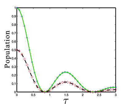
Figure 1: (Color online) Time evolution of the population in the upper level for different initial states (a) $|\ {\phi_{1}}\rangle=|\ e\rangle$ and (b) $|\ {\phi_{2}}\rangle=(|\ e\rangle+|\ g\rangle)/\sqrt{2}\,,$ ($\tau=\lambda t$), both with $\lambda=1$, $\gamma_{0}=10$, for the cases of (i) the numerical solution of TCL master equation for initial state $|\ {\phi_{1}}\rangle=|\ e\rangle$ (asterisk), (ii) the exact analytical solution for initial state $|\ {\phi_{1}}\rangle=|\ e\rangle$ (solid curve), (iii) the numerical solution of TCL master equation for initial state $|\ {\phi_{2}}\rangle=(|\ e\rangle+|\ g\rangle)/\sqrt{2}$ (diamond), and (iv) the exact analytical solution for initial state $|\ {\phi_{2}}\rangle=(|\ e\rangle+|\ g\rangle)/\sqrt{2}$ (dashed curve).

II.1 Validity of TCL master equation

One problem for the TCL master equation is that it was thought to break down at finite time in strong-coupling regime due to the singularity. For example, the problem occurs in the case that the spectral density of the reservoir takes the Lorentzian form $J(\omega_{k})=\gamma_{0}\lambda^{2}/2\pi[(\omega_{k}-\omega_{c})^{2}+\lambda^{2}]$ and the two-level system interacts with the central frequency of the reservoir resonantly, $\omega_{0}=\omega_{c}$ QO1 ; GME . In the following, we restudy this problem for this model. If $\omega_{c}\gg\lambda$, such as in an optical cavity, $\omega_{c}$ can be extended to infinity. Then the correlation function $f(t-\tau)$ is given by

$$f(t-\tau)=\frac{{\gamma_{0}\lambda}}{2}e^{-\lambda|{t-\tau}|}\,.$$ (5)

Substituting Eq. (5) into (2) and using Laplace approach, one obtains QO1

$$c_{e}(t)=c_{e0}e^{-\lambda t/2}\left[{\cos\left({\frac{{\Gamma}}{2}t}\right)+\frac{\lambda}{\Gamma}\sin\left({\frac{{\Gamma}}{2}t}\right)}\right]\,,$$ (6)

where $\Gamma=\sqrt{2\gamma_{0}\lambda-\lambda^{2}}$. For the strong-coupling case ($\gamma_{0}>\lambda/2$), $\Gamma>0$, and $c_{e}(t)$ is an oscillating function with discrete zeros at $t_{n}=2[{(n+1)\pi-\arctan(\Gamma/\lambda)}]/\Gamma$, ($n=0,1,2,\cdots$). Substituting Eq. (6) into (4), one obtains the exact expressions for $S(t)$ and $\gamma(t)$ GME

$$S(t)=0,\ \ \gamma(t)=\frac{2\gamma_{0}\tan(\Gamma t/2)}{1+\lambda/\Gamma\tan(\Gamma t/2)}.$$ (7)

Therefore, we see that $\gamma(t)$ diverges at these points $t_{n}$.

Previously, it was generally thought that the singularity is an obstacle for validity of the TCL master equation QO1 ; GME . On one hand, for TCL master equation, since “the evolution of the reduced density matrix only depends on the actual value of $\rho_{s}(t)$ and on the TCL generator” QO1 and the density matrices coincide at $t=t_{0}$ for different initial states, the evolution of the density matrices after $t_{0}$ should be the same for different initial states. On the other hand, the exact analytical solution QO1 for the problem shows that the density matrices for $t>t_{0}$ differs for different initial states. That means the solution of TCL master equation does not agree with the exact analytical solution for $t>t_{0}$. So, it was thought that, “…a time-convolutionless form of the equation of motion which is local in time ceases to exist for $t>t_{0}$…” QO1 or “…the time-convolutionless generator breaks down at finite time in the strong coupling regime, thus failing to reproduce the asymptotic behavior…” GME .

In our opinion, the singularity is not an obstacle for validity of the TCL master equation. By using the method in NMQJ , we solve the TCL master equation Eq. (3) numerically. In the simulation, the decay rate (Eq. (7)) with singularity is used. From Fig. 1, we find that the numerical solution of TCL master equation agrees with the exact analytical solution very well for $t>t_{0}$. That means, even though the TCL master equation has a singular point at $t=t_{0}$ in strong-coupling regime, it still reproduces the correct dynamics when $t>t_{0}$. Actually, since $t=t_{0}$ is a singulary point of the TCL master equation, the dynamics around $t=t_{0}$ cannot be explained by the theory of the first-order ordinary differential equation at an ordinary point ODE .

II.2 Multiscale perturbative expansion

Another crucial problem for TCL master equation is that the ordinary perturbative expansion fails in strong-coupling regime QO1 . The reason is that the ordinary perturbative expansion corresponds basically to a Taylor expansion of $\gamma(t)$ in powers of $\gamma_{0}$. In fact, this method treats the dynamics only in one time scale. For the model considered above in strong-coupling regime, there are two time scales, which correspond to the decaying and the oscillating behaviors, respectively. The ordinary perturbative expansion only considers the time scale of the decaying behavior, so the oscillating behavior disappears in the perturbative solution (see Fig. 2).

Figure 2: (Color online) Time evolution of the population in the upper level for initial state $|\ e\rangle$ by multiscale perturbative method and ordinary perturbative method ($\tau=\lambda t$), with $\lambda=1$, $\gamma_{0}=10$, for the cases of (i) the exact solution (solid curve), (ii) the numerical solution of exact TCL master equation (cross), (iii) the first order multiscale method (diamond), (iv) the second order multicale method (asterisk), (v) the second order ordinary perturbative method (dash-dotted curve), (vi) the fourth order ordinary perturbative method (dotted curve).

Since the failure of the ordinary perturbative expansion originates from ignoring multiscales of the dynamics, we introduce a multiscale perturbative expansion Multi to treat the strong-coupling case.

According to Eq. (4), by giving a multiscale perturbative expansion of $c_{e}(t)$, one can get the multiscale perturbative expansions of $\gamma(t)$ and $S(t)$. From Eqs. (2) and (5), one obtains

$$\ddot{c}_{e}(t)+\lambda\dot{c}_{e}(t)+\frac{{\gamma_{0}\lambda}}{2}c_{e}(t)=0\,.$$ (8)

By introducing dimensionless parameters $T=\gamma_{0}t$ and $\varepsilon{\rm{=}}\lambda{\rm{/}}\gamma_{0}$, where $\varepsilon\ll 1$ for strong-coupling regime, Eq. (8) reads

$$\frac{{d^{2}}}{{dT^{2}}}c_{e}+\varepsilon\frac{d}{{dT}}c_{e}+\frac{\varepsilon}{2}c_{e}=0\,,$$ (9)

with initial conditions $c_{e}(0)=c_{e0}$ and $\dot{c}_{e}(0)=0$. There are two kinds of behaviors of the dynamics, corresponding to two different time scales. The time scale of the decaying behavior relates to $\lambda t=\varepsilon T$, and that of the oscillating behavior relates to a complicated function of $\varepsilon$. Therefore, two different time scales, $t_{1}=(\varepsilon^{1/2}a_{1}+\varepsilon^{3/2}a_{2}+...)T$ and $t_{2}=\varepsilon T$, are introduced, where $a_{i}$’s are unknown parameters to be determined. Expanding $c_{e}(t_{1},t_{2})$ in powers of $\varepsilon$

$$c_{e}(t_{1},t_{2})=c_{e}^{(0)}(t_{1},t_{2})+\varepsilon^{1/2}c_{e}^{(1)}(t_{1},t_{2})+\varepsilon c_{e}^{(2)}(t_{1},t_{2})+...\,,$$ (10)

and substituting Eq. (10) into (9) and the initial conditions, one obtains the equations for $c_{e}^{(i)}$ as follows.

To the order of $\varepsilon$, one gets the equations for $c_{e}^{(0)}$ as

$$a_{1}^{2}\frac{{\partial^{2}}}{{\partial t_{1}^{2}}}c_{e}^{(0)}+\frac{1}{2}c_{e}^{(0)}=0\,,$$

$$c_{e}^{(0)}(0,0)=c_{e0},\ \ \frac{\partial}{{\partial t_{1}}}c_{e}^{(0)}(0,0)=0\,.$$

To the order of $\varepsilon^{3/2}$, one gets the equations for $c_{e}^{(1)}$ as

$$a_{1}^{2}\frac{{\partial^{2}}}{{\partial t_{1}^{2}}}c_{e}^{(1)}+\frac{1}{2}c_{e}^{(1)}=-2a_{1}\frac{{\partial^{2}}}{{\partial t_{1}\partial t_{2}}}c_{e}^{(0)}-a_{1}\frac{\partial}{{\partial t_{1}}}c_{e}^{(0)}\,,$$

$$c_{e}^{(1)}(0,0)=0\,,$$

$$a_{1}\frac{\partial}{{\partial t_{1}}}c_{e}^{(1)}(0,0)+\frac{\partial}{{\partial t_{2}}}c_{e}^{(0)}(0,0)=0\,.$$

To the order of $\varepsilon^{2}$, one gets the equations for $c_{e}^{(2)}$ as

$$a_{1}^{2}\frac{{\partial^{2}}}{{\partial t_{1}^{2}}}c_{e}^{(2)}+\frac{1}{2}c_{e}^{(2)}=-2a_{1}\frac{{\partial^{2}}}{{\partial t_{1}\partial t_{2}}}c_{e}^{(1)}-2a_{1}a_{2}\frac{{\partial^{2}}}{{\partial t_{1}^{2}}}c_{e}^{(0)}$$

$$\qquad-\frac{{\partial^{2}}}{{\partial t_{2}^{2}}}c_{e}^{(0)}-a_{1}\frac{\partial}{{\partial t_{1}}}c_{e}^{(1)}-\frac{\partial}{{\partial t_{2}}}c_{e}^{(0)}\,,$$

$$c_{e}^{(2)}(0,0)=0\,,$$

$$a_{1}\frac{\partial}{{\partial t_{1}}}c_{e}^{(2)}(0,0)+a_{2}\frac{\partial}{{\partial t_{1}}}c_{e}^{(0)}(0,0)+\frac{\partial}{{\partial t_{2}}}c_{e}^{(1)}(0,0)=0\,.$$

By a routine multiscale analysis of the above equations Multi , one obtains the solutions of $c_{e}^{(i)}$. By substituting the perturbative solution of $c_{e}$ into Eq. (4), we can get the corresponding Lamb shifts and decay rates. The first order solution is

$$S(t)=0,\ \ \gamma(t)=\varepsilon+\sqrt{2\varepsilon}\tan(\sqrt{2\varepsilon}T/2),$$

and the second order solution is

$$S(t)=0,\ \ \ \ \ \ \ \ \ \ \ \ \gamma(t)=\frac{{\sqrt{\varepsilon}\{\varepsilon^{3/2}\cos[\sqrt{2\varepsilon}(1-\varepsilon/4)T/2]+\sqrt{2}(4+\varepsilon)\sin[\sqrt{2\varepsilon}(1-\varepsilon/4)T/2]\}}}{{4\cos[\sqrt{2\varepsilon}(1-\varepsilon/4)T/2]+2\sqrt{2\varepsilon}\sin[\sqrt{2\varepsilon}(1-\varepsilon/4)T/2]}}.$$

By solving the corresponding master equations using the method in NMQJ , we study the dynamics of the population in the upper level. From Fig. 2, we can see that, unlike the solutions of ordinary perturbative method where the oscillating behavior is missing, the decaying and oscillating behaviors are both included by multiscale perturbative solutions. The perturbative solution up to the second order fits very well with the exact solution.

For the exact solution, Eq. (7), the first singular time of $\gamma(t)$ is $t_{0}=2\arccos(-\sqrt{\varepsilon/2})/[\gamma_{0}\sqrt{(2-\varepsilon)\varepsilon}]$. For the first and second order approximations of $t_{0}$ by the multiscale perturbative expansion, the first singular time of $\gamma(t)$ are $\pi/[\gamma_{0}\sqrt{2\varepsilon}]$ and $4\sqrt{2}\arccos[-\sqrt{\varepsilon/(2+\varepsilon)}]/[\gamma_{0}(4-\varepsilon)\sqrt{\varepsilon}]$, respectively. Detailed analysis shows that relative errors of the first and second order approximations are in the orders of $\varepsilon^{1/2}$ and $\varepsilon^{3/2}$, respectively.

III Conclusion

To summarize, we study the time-convolutionless non-Markovian master equation in strong-coupling regime. For the environment with Lorentzian spectral density, we find that the singularity at finite time does not influence the master equation to produce the correct asymptotic behavior of the open system. We also propose a multiscale perturbative method, which fits well with the exact solution, though the ordinary perturbative method fails, in strong-coupling regime.

References

- (1) T. Yu and J.H. Eberly, Phys. Rev. Lett. 93, 140404 (2004); T. Yu and J.H. Eberly, ibid. 97, 140403 (2006); T. Yu and J.H. Eberly, Science 323, 598 (2009); B. Bellomo, R.L. Franco and G. Compagno, Phys. Rev. Lett. 99, 160502 (2007); Y. Li, J. Zhou, and H. Guo, Phys. Rev. A 79, 012309 (2009); L. Mazzola, J. Piilo, and S. Maniscalco, Phys. Rev. Lett. 104, 200401 (2010).
- (2) H.-P. Breuer and F. Petruccione, The Theory of Open Quantum Systems (Oxford University Press, Oxford, 2002).
- (3) C.W. Gardiner and P. Zoller, Quantum Noise (Springer-Verlag, Berlin, 1999).
- (4) P. Lambropoulos et al., Rep. Prog. Phys. bf 63, 455 (2000).
- (5) See e.g., C.W. Lai, P. Maletinsky, A. Badolato, and A. Imamoglu, Phys. Rev. Lett. 96, 167403 (2006), and references therein.
- (6) K.H. Madsen, et. al., Phys. Rev. Lett. 106, 233601 (2011).
- (7) J. Shao, J. Chem. Phys. 120, 5053 (2004); A. Pomyalov and D.J. Tannor, ibid. 123, 204111 (2005), and references therein.
- (8) P. Rebentrost, R. Chakraborty, and A. Aspuru-Guzik, J. Chem. Phys. 131, 184102 (2009).
- (9) S. Nakajima, Progr. Theor. Phys. 20, 948 (1958); R. Zwanzig, J. Chem. Phys. 33, 1338 (1960).
- (10) F. Shibata, Y. Takahashi, and N. Hashitsume, J. Stat. Phys. 77, 171 (1977); F. Shibata and T. Arimitsu, J. Phys. Soc. Jap. 49, 891 (1980).
- (11) W.T. Strunz, Phys. Lett. A 224, 25 (1996); L. Disi and W.T. Strunz, Phys. Lett. A 235, 569 (1996); L. Disi, N. Gisin, and W.T. Strunz, Phys. Rev. A 58, 1699 (1998); W.T. Strunz, L. Disi, and N. Gisin, Phys. Rev. Lett. 82,1801 (1999).
- (12) B.M. Garraway, Phys. Rev. A 55, 2290 (1997).
- (13) H.-P. Breuer, B. Kappler, and F. Petruccione, Phys. Rev. A 59, 1633 (1999).
- (14) H.-P. Breuer, Phys. Rev. A 70, 012106 (2004).
- (15) J. Piilo, S. Maniscalco, K. Hrkonen, and K.-A. Suominen, Phys. Rev. Lett. 100, 180402 (2008).
- (16) C.J. Wu, Y. Li, M.Y. Zhu, and H. Guo, Phys. Rev. A 83, 052116 (2011).
- (17) B. Vacchini and H.-P. Breuer, Phys. Rev. A 81, 042103 (2010).
- (18) Q.-J. Tong, J.-H. An, H.-G. Luo, and C.H. Oh, Phys. Rev. A 81, 052330 (2010).
- (19) E.A. Coddington and N. Levinson, Theory of Ordinary Differential Equations (McGraw-Hill, New York, 1955).
- (20) D. Zwillinger, Handbook of Differential Equations (Academic Press, San Diego, 1989).