Density preturbations in a finite scale factor singularity universe

Abstract

We discuss evolution of density perturbations in cosmological models which admit finite scale factor singularities. After solving the matter perturbations equations we find that there exists a set of the parameters which admit a finite scale factor singularity in future and instantaneously recover matter density evolution history which are indistinguishable from the standard $\Lambda$CDM scenario.

I Introduction

One of the most problematic phenomena resulting from observations of high-redshift type Ia supernovae (SNIa) is recent accelerated expansion of the universe. Search for the explanation of this phenomena led physicists to many various possible cosmological scenarios based on different approaches like modifying physical expansion history or modifying the theory of gravity. Out of this effort there arised a couple of cosmological scenarios. Some of them admit new types of singularities which has already not been known, within the framework of the so-called standard or concordance cosmology. Finite scale factor singularities (FSF) are one of the types and were first found in Ref. nojiri . Basically, it is assumed that the universe is accelerating due to an unknown form of energy supernovaeold which phenomenologically behaves as the cosmological constant. More observational data supernovaenew made cosmologists think of an accelerating universe filled with phantom phantom which violated all energy conditions: the null ($\varrho+p\geq 0$), weak ($\varrho\geq 0$ and $\varrho+p\geq 0$), strong ($\varrho+p\geq 0$ and $\varrho+3p\geq 0$), and dominant energy ($\varrho\geq 0$, $-\varrho\leq p\leq\varrho$) ($\varrho$ is the energy density and $p$ is the pressure). A phantom-driven dark energy leads to a big-rip singularity (BR, or type I according to nojiri ) in which the infinite values of the energy density and pressure ($\rho$, $p\to\infty$) are accompanied by the infinite value of the scale factor ($a\to\infty$) caldwellPRL .

The list of new types of singularities contains: a big-rip (BR) phantom , a sudden future singularity (SFS) sahni ; barrow04 ; barrow042 ; no0408170 ; Bambaetal ; sfs1 , a generalized sudden future singularity (GSFS), a finite scale factor singularity (FSF) aps , a big-separation singularity (BS) and a $w$-singularity wsin . A weaker version of the Big-Rip such as a Little-Rip and a Pseudo-Rip has also been proposed recently littlerip ; pseudorip . In this paper we deal with a finite scale factor singularity. This is a weak singularity according to Tipler and a strong singularity according to Królak lazkoz .

In Ref. fsf we found that there is a set of the parameters which, within the $1\sigma$ CL, fits the observational data BAO, SNIa and the shift parameter, and admits an FSF singularity. In this paper we deal with the problem of growth of density perturbations in the scenario admitting such a singularity.

The paper is organized as follows. In section II we present an FSF scenario. In section III we present the expressions for the evolution of linear density perturbations of matter in general relativity, and rewrite them for the scenario admitting an FSF singularity. In section IV we give the results and discussion.

II A Finite Scale Factor Singularity Universe

In order to obtain an FSF singularity one should start with the simple framework of an Einstein-Friedmann cosmology governed by the standard field equations (we assumed flat universe)

$$\rho = \frac{3}{8\pi G}\left(\frac{\dot{a}}{a}\right)^{2}~{},$$ (II.1)

$$p = -\frac{1}{8\pi G}\left(2\frac{\ddot{a}}{a}+\frac{\dot{a}^{2}}{a^{2}}\right)~{}.$$ (II.2)

Similarly like in the case of an SFS, which were tested against the observations in Refs. DHD ; GHDD ; DDGH , one is able to obtain an FSF singularity by taking the scale factor in the form

$$a(y)=a_{s}\left[\delta+\left(1-\delta\right)y^{m}-\delta\left(1-y\right)^{n}\right]~{},\hskip 14.22636pty\equiv\frac{t}{t_{s}}$$ (II.3)

with the appropriate choice of the constants $\delta,t_{s},a_{s},m,n$. In contrast to an SFS, in order to have an accelerated expansion of the universe, $\delta$ has to be positive ($\delta>0$). For $1<n<2$ we have an SFS. In order to have an FSF singularity instead of SFS, $n$ has to be limited to $0<n<1$.

As can be seen from (II.1)-(II.3), for an FSF $\rho$ diverges and we have $a\rightarrow a_{s}$, $\rho\rightarrow\infty$, and $|p|\rightarrow\infty$ for $t\rightarrow t_{s}$.
In the model (II.3), the evolution begins with a standard big-bang singularity at $t=0$ for $a=0$, and finishes at a finite scale factor singularity at $t=t_{s}$, where $a=a_{s}\equiv a(t_{s})$ is a constant. In terms of the rescaled time $y$, we have $a(1)=a_{s}$.

The standard Friedmann limit (i.e. models without an FSF singularity) of (II.3) is achieved when $\delta\to 0$; hence $\delta$ is called the “non-standardicity” parameter. Additionally, notwithstanding Ref. barrow04 , and in agreement with the field equations (II.1)-(II.3), $\delta$ can be both positive and negative leading to an acceleration or a deceleration of the universe, respectively.
To our discussion it is important that the asymptotic behaviour of the scale factor (II.3) close to a big-bang singularity at $t=0$ is given by a simple power-law $a_{\rm BB}=y^{m}$, simulating the behaviour of flat ($k=0$) barotropic fluid models with $m=2/[3(w+1)]$ where $w$ is barotropic index ($p=w\rho$).
Recently, an FSF singularity scenario was confronted with baryon acoustic oscillations, distance to the last scattering surface, and SNIa fsf . It was shown that for a finite scale factor singularity there is an allowed value of $m=2/3$ within $1\sigma$ CL, which corresponds to a dust-filled Einstein-de-Sitter universe in the past. It was also shown that an FSF singularity may happen within $2\times 10^{9}$ years in future in $1\sigma$ confidence level, and its observational predictions at the present moment of cosmic evolution cannot be distinguished from the predictions given by the standard quintessence scenario of future evolution in the Concordance Model chevallier00 ; linder02 ; linder05 ; koivisto05 ; caldwell07 ; zhang07 ; amendola07 ; diporto07 ; hu07b ; linder09 .

III Linear density perturbations

In the linear regime the equations that govern the evolution of perturbations in a Friedmann universe consisting of more than one component constitute a complicated set of coupled differential equations mukhanov . In this paper we consider the evolution of perturbations in a flat Friedmann universe made up of a dust matter with the density $\rho_{m}$ and a dark energy with density $\rho_{de}$, and pressure $p_{de}$. It was shown in christopherson that, in similar case, neglecting perturbations in dark energy one makes some particular, unintended choice of gauge and in general that may lead to errorneous results for perturbations in the matter. Taking that into account we restrict our investigations to the cases where the proper wavelength of perturbations is much smaller than the Hubble radius and the sound velocity for the dark energy has a positive value of order of unity, while the barotropic index for the dark energy is a reasonable slowly varying function of the cosmic time. With these assumptions the dark matter perturbations effectively decouple from perturbations in the dark energy and the evolution of the matter density contrast $\delta_{m}$ can be described to a good approximation with the following equations:

$$\ddot{\delta}_{m}+2H\dot{\delta}_{m} = 4\pi G\rho_{m}\delta_{m},$$ (III.1)

$$\left(\frac{\dot{a}}{a}\right)^{2} = \frac{8\pi G}{3}(\varrho_{m}+\varrho_{de})$$ (III.2)

$$2\frac{\ddot{a}}{a}+\left(\frac{\dot{a}}{a}\right)^{2} = -8\pi Gp_{de},$$ (III.3)

where a dot denotes a derivative with respect to time $H=\dot{a}/a$ is the Hubble parameter.
Since the amplitude of the anisotropy is determined by the typical amplitude of peculiar velocities and those, in the linear theory, correspond to growth rate of perturbations $f=d\ln\delta/d\ln a$, we will write down the equation (III.1) in terms of this logarithmic growth rate as follows:

$$\frac{df}{dx}+f^{2}+\left(\frac{\dot{H}}{H^{2}}+2\right)f-\frac{3}{2}\Omega_{m}=0,$$ (III.4)

where $dx=d\ln a$ and

$$\Omega_{m}=\Omega_{0m}\frac{H_{0}^{2}a_{0}^{3}}{H{{}^{2}}a^{3}}.$$ (III.5)

Further, taking the scale factor (II.3), we get the equation for the growth rate evolution in the form:

$$\frac{a}{a^{\prime}}f^{\prime}-f^{2}+\left(1+\frac{aa^{\prime\prime}}{a^{\prime 2}}\right)f-\frac{3}{2}\Omega_{m}=0,$$ (III.6)

where $\prime$ denotes derivative with respect to $y$ from (II.3) and

$$\Omega_{m}=\Omega_{0m}\frac{a_{0}^{3}\mathcal{H}_{0}^{2}}{a^{3}\mathcal{H}^{2}},$$ (III.7)

where $\mathcal{H}=a_{0}^{\prime}/a_{0}$ and $a_{0}=a(y_{0})$.
Observational data from Lyman-$\alpha$ forests and galaxy redshift distortions for the growth rate $f$, to which we fit our model, are given in table 1.

$z$	$f_{obs}$
$0.15$	$0.51\pm 0.11$
$0.35$	$0.7\pm 0.18$
$0.55$	$0.75\pm 0.18$
$1.4$	$0.9\pm 0.24$
$3.0$	$1.46\pm 0.29$

Table 1: Observational data for the growth factor $f$ from Lyman-$\alpha$ forests and galaxy redshift distortions taken from Refs guzzo ; colless ; tegmark ; ross ; angela ; mcdonald .

IV Results and Conclusions

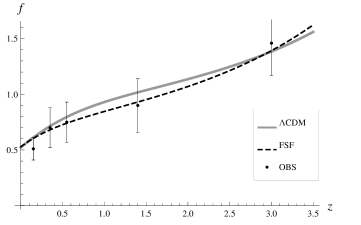
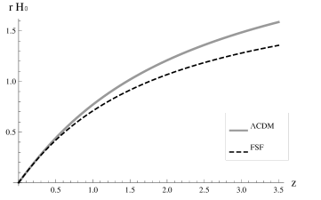
Figure 1: Upper left panel presents the predicted growth rate plotted against redshift for an FSF model (dashed line) and a $\Lambda$CDM model (solid line). There are also shown the observed data points (dots) for the growth rate. The upper right panel shows the distance-redshift relation for both FSF and $\Lambda$CDM models. The left and right bottom panels present the corresponding relative errors.

The main goal of this paper is to find the fit to currently available data for the growth of perturbations rate taken from Refs. guzzo ; colless ; tegmark ; ross ; angela ; mcdonald (see table 1) for the cosmological model which admits an FSF singularity. We are searching for the fit, varying the model parameters which are $m$, $n$, $\delta$, $y_{0}$, $f_{0}$, and the last parameter $f_{0}$ is the present value of the growth rate $f$. We search for such a set of the parameters that satisfies, within $1\sigma$ CL, BAO, SNIa, and the shift parameter data as well (see fsf ).
We solve the equation (III.6) numerically for a given set of the parameters using the standard Runge-Kutta method with an adaptative step size. Applying a standard Levenberg-Marquardt method, we search for the minimum of the $\chi^{2}$ function which is of the form

$$\chi^{2}(z;\mathbf{p})=\sum_{i=1}^{5}\frac{(f_{obs}(z_{i};\mathbf{p})-f_{th}(z_{i};\mathbf{p}))^{2}}{\sigma_{i}^{2}},$$ (IV.1)

where: $f_{obs}$ and $\sigma_{i}$ are taken from the table 1; $f_{th}$ is calculated by solving the equation (III.6); $\mathbf{p}\equiv(m,n,\delta,y_{0},f_{0})$. We find the following fit for one of the possible set of parameters:

$$y_{0}=0.55,\ \delta=0.67,\ m=0.49,\ n=0.32,\ f_{0}=0.53,$$

with $\chi^{2}=0.99$. For this set of parameters we evaluate the growth rate function $f$, again solving numerically eq. (III.6), cf. the upper left panel of figure 1. In this panel together with growth rate for FSF scenario, we see the growth rate for $\Lambda$CDM scenario and the measured values of the growth rate with their errorbars. In a bottom left panel we see the relative difference between the evaluation of the growth rate function, for an FSF scenario and for a $\Lambda$CDM. The discrepancy for both models is at most $9\%$ for $z\sim 1$.
In the top right panel of the figure 1 we see the distance-redshift relation for an FSF scenario and a $\Lambda$CDM model. In the bottom right panel of the same plot we see a relative difference between distance-redshift relations for both models, which is biggest ($14\%$) for the most distant values of $z\sim 3.5$.
As in Refs. fsf and DDGH , the set of the parameters that we obtained was tested against several additional conditions, what assured, that some other physical conditions are satisfied which are listed bellow:

• we assumed that, the scale factor and its first derivative for all times is always positive, i.e. $a(y)>0$, and $\dot{a}(y)>0$;

• a current expansion of the universe should be accelerated, i.e. $\ddot{a}(y_{0})>0$;

• time should be decaying function of $z$, positive redshift should correspond to the past ($z>0$ for $y<y_{0}$) and negative redshift should correspond to the future ($z<0$ for $y>y_{0}$).

We conclude that for the FSF models there exists a set of parameters which fits the observational data for the growth rate and on the other hand satisfies, within $1\sigma$ CL, the data for BAO, SNIa and the shift parameter. Thus we proved that current observations are incapable of ruling out FSF models of the expanding universe.

V Acknowledgements

We acknowledge the support of the National Science Center grant No N N202 3269 40 (years 2011-2013).

References

- (1) S. Nojiri, S.D. Odintsov and S. Tsujikawa, Phys. Rev. D 71,063004 (2005).
- (2) S. Perlmutter et al., Astroph. J. 517, (1999) 565; A. G. Riess et al., Astron. J. 116, 1009 (1998); A.G. Riess et al., Astroph. J. 560, 49 (2001).
- (3) J.L. Tonry et al., Astroph. J. 594, 1 (2003); M. Tegmark et al., Phys. Rev. D69, 103501 (2004); R.A. Knop et al., Astrophys. J. 598, 102 (2003).
- (4) R.R. Caldwell, Phys. Lett. B 545, 23 (2002); M.P. Da̧browski, T. Stachowiak and M. Szydłowski, Phys. Rev. D 68, 103519 (2003); P.H. Frampton, Phys. Lett. B 562 (2003), 139; H. Štefančić, Phys. Lett. B586, 5 (2004); E. Elizalde, S. Nojiri and S. D. Odintsov, Phys. Rev. D70, 043539 (2004); S. Nojiri and S.D. Odintsov, Phys. Lett. B595, 1 (2004).
- (5) R.R. Caldwell, M. Kamionkowski, and N.N. Weinberg, Phys. Rev. Lett. 91, 071301 (2003).
- (6) V. Sahni and Yu.V. Shtanov, Class. Quantum Grav. 19, L101 (2002).
- (7) J.D. Barrow, Class. Quantum Grav. 21, L79 (2004).
- (8) J.D. Barrow and Ch. Tsagas, Class. Quantum Grav. 22, 1563 (2005).
- (9) S. Nojiri and S. D. Odintsov, Phys. Rev. D 70, 103522 (2004).
- (10) K. Bamba, S. Nojiri, and S. D. Odintsov, J. Cosmol. Astropart. Phys. 10 (2008) 045.
- (11) M.P. Da̧browski, Phys. Rev. D71, 103505 (2005).
- (12) M.P. Da̧browski and T. Denkiewicz, AIP Conference Proceedings 1241, 561 (2010).
- (13) T. Denkiewicz, arXiv:1112.5447.
- (14) L. Fernandez-Jambrina and R. Lazkoz, Phys. Rev. D70, 121503(R) (2004); L. Fernandez-Jambrina and R. Lazkoz, Phys. Rev. D74, 064030 (2006).
- (15) M.P. Da̧browski and T. Denkiewicz, Phys. Rev. D79, 063521 (2009).
- (16) P. H. Frampton, K. J. Ludwick, R. J. Scherrer, Phys.Rev. D84, 063003 (2011).
- (17) P. H. Frampton, K. J. Ludwick, R. J. Scherrer, arXiv:1112.2964v1 .
- (18) A. A. Starobinsky, Phys. Lett. 91B, 99 (1980).
- (19) M. R. Setare and E. N. Saridakis, Phys. Lett. B671, 331 (2009).
- (20) V. Sahni and Yu. Shtanov, Phys. Rev. D 71, 084018 (2005).
- (21) M. P. Dabrowski, T. Denkiewicz, M. A. Hendry, Phys. Rev. D75, 123524 (2007).
- (22) H. Ghodsi, M. A. Hendry, M. P. Dabrowski, T. Denkiewicz, MNRAS, 414: 1517–1525 (2011).
- (23) Tomasz Denkiewicz, Mariusz P. Dcabrowski, Hoda Ghodsi, Martin A. Hendry, arXiv:1201.6661
- (24) M. Chevallier and D. Polarski, Int. J. Mod. Phys. D10, 213 (2001).
- (25) E. V. Linder, Phys. Rev. Lett. 90, 091301 (2003).
- (26) E. V. Linder, Phys. Rev. D72, 043529 (2005).
- (27) T. Koivisto and D. F. Mota, Phys. Rev. D73, 083502 (2006).
- (28) R. Caldwell, A. Cooray and A. Melchiorri, Phys. Rev. D76, 023507 (2007).
- (29) P. Zhang, M. Liguori, R. Bean and S. Dodelson, Phys. Rev. Lett. 99, 141302 (2007).
- (30) A. J. Christopherson Phys. Rev. D82, 083515 (2010).
- (31) L. Amendola, M. Kunz and D. Sapone, JCAP 0804, 013 (2008).
- (32) C. Di Porto and L. Amendola, Phys. Rev. D77, 083508 (2008).
- (33) W. Hu and I. Sawicki, Phys. Rev. D76, 104043 (2007).
- (34) E. V. Linder, Phys. Rev. D79, 063519 (2009).
- (35) L. Guzzo et al., Nature 451, 541 (2008).
- (36) M. Colless et al., Mont. Not. R. Astron. Soc. 328, 1039 (2001).
- (37) M. Tegmark el al., Phys. Rev. D 74, 123507 (2006).
- (38) N.P. Ross et al., Mont. Not. R. Astron. Soc. 381, 573 (2007).
- (39) J. da Ângela et al., Mont. Not. R. Astron. Soc. 383, 565 (2008).
- (40) P. McDonald et al., Astrophys. J. 635, 761 (2005).
- (41) V. F. Mukhanov, H. A. Feldman and R. H. Brandenberger, Phys. Rep. 205, 215 (1992).