Simultaneous $B^{\prime}V^{\prime}R^{\prime}$ Monitoring of BL Lacertae Object S5 0716+714 and Detection of Inter-Band Time Delay

Abstract

We present the results of our optical monitoring of the BL Lac object S5 0716+714 on seven nights in 2006 December. The monitoring was carried out simultaneously at three optical wavelengths with a novel photometric system. The object did not show large-amplitude internight variations during this period. Intranight variations were observed on four nights and probably on one more. Strong bluer-when-brighter chromatism was detected on both intranight and internight timescales. The intranight variation amplitude decreases in the wavelength sequence of $B^{\prime}$, $R^{\prime}$, and $V^{\prime}$. Cross correlation analyses revealed that the variability at the $B^{\prime}$ and $V^{\prime}$ bands lead that at the $R^{\prime}$ band by about 30 minutes on one night.

1 INTRODUCTION

Blazars represent the most violently variable objects among all active galactic nuclei (AGNs). They show rapid and strong variability, high and variable polarization, and a non-thermal continuum. The variable continuum is believed to come from near the base of the relativistic jet closely aligned with our light of sight. The jet is probably powered and accelerated by a rotating supermassive black hole surrounded by an accretion disk. A blazar can either be termed as a flat-spectrum radio quasar (FSRQ) or a BL Lac object, depending on whether or not it shows strong emission lines in its spectrum.

The spectral energy distribution (SED) of blazars has a two-bumped structure: The low-frequency bump ranges from radio to UV or X-ray frequencies and is believed to come from the synchrotron emission from the relativistic electrons in the jet. The high-frequency bump, from X-rays to $\gamma$-rays, is usually interpreted as emission from inverse Compton scattering of the low frequency radiation by the same ensemble of relativistic electrons responsible for the synchrotron emission (for a recent review, see Böttcher, 2007). According to the peak frequency of their synchrotron emission, BL Lac objects can be further divided into low-frequency-peaked BL Lacs (LBL) and high-frequency-peaked BL Lacs (HBL). The former subclass has the synchrotron peak at IR–optical wavelengths while the latter subclass has the peak in the UV or soft X-ray band.

The BL Lac object S5 0716+714, probably at a redshift of 0.31$\pm$0.08 (Nilsson et al., 2008), is one of the best studied blazars. It is highly variable from radio to X-ray (Wagner et al., 1996) and $\gamma$-ray wavelengths (Lin et al., 1995; Chen et al., 2008). Most recently, MAGIC detected very high energy $\gamma$-ray emission from this object(Anderhub et al., 2009). Its SED has been observed and studied by a number of multi-wavelength campaigns (e.g., Giommi et al., 1999, 2008; Tagliaferri et al., 2003; Ferrero et al., 2006; Foschini et al., 2006; Ostorero et al., 2006; Villata et al., 2008). The majority of the observations revealed a two-bumped structure of the SED with a concave shape at 2 – 3 keV. Furthermore, it was found that its emission from radio to soft X-rays, likely due to the synchrotron process, could be highly variable, while the hard X-ray (from 3 to 10 keV) flux, most probably dominated by inverse Compton emission, usually remained constant. A model with two synchrotron self-Compton (SSC) components was proposed to explain its SED changes, with one component highly variable and the other constant (Chen et al., 2008; Giommi et al., 2008).

In the optical regime, S5 0716+714 is one of the brightest blazars. It has a duty cycle close to 1, which means that it almost never stops its variation (e.g., Wagner & Witzel, 1995; Stalin et al., 2009; Chandra et al., 2011). Its optical variability has been studied on different timescales by a number of authors (Ghisellini et al., 1997; Sagar et al., 1999; Villata et al., 2000; Nesci et al., 2002, 2005; Qian et al., 2002; Raiteri et al., 2003; Xie et al., 2004; Wu et al., 2005, 2007a; Montagni et al., 2006; Stalin et al., 2006; Pollock et al., 2007; Gupta et al., 2008; Sasada et al., 2008; Zhang et al., 2008; Stalin et al., 2009; Poon et al., 2009; Zhang et al., 2010a; Carini et al., 2011; Chandra et al., 2011). Its variation rate can be faster than 0.10-0.12 $\rm{mag\,hr^{-1}}$ (Sagar et al., 1999; Villata et al., 2000; Wu et al., 2005; Montagni et al., 2006). A maximum rate of 0.16 $\rm{mag\,hr^{-1}}$ was reported by Nesci et al. (2002). The variation timescale can be as short as 15 minutes (Sasada et al., 2008; Rani et al., 2010a; Chandra et al., 2011). Most recently, Fan et al. (2011) even reported a 0.611 mag variation over 3.6 minutes in this object.

The color or spectral behavior of blazars is a subject of much debates. Some authors found a bluer-when-brighter (BWB) chromatism (e.g., Vagnetti et al., 2003), some others claimed the opposite behavior, namely, a redder-when-brighter (RWB) trend (e.g., Ramírez et al., 2004), or no clear tendency (e.g., Böttcher et al., 2007, 2009). It appears that BL Lacs are BWB while FSRQs are RWB (Fan & Lin, 2000; Gu et al., 2006; Hu et al., 2006; Rani et al., 2010b). A certain object may display different trends in different variation modes (e.g., Wu et al., 2005; Poon et al., 2009) or on different timescales (e.g., Ghisellini et al., 1997; Raiteri et al., 2003). One reason for these divergences is that almost all previous observations were done quasi-simultaneously at multiple wavelengths. When the exposure was switched from one wavelength to the other, the brightness of the source might have changed. So the quasi-simultaneous observations cannot obtain real color, and the color behavior drawn from these observations should be taken with caution.

We monitored S5 0716+714 for seven nights in 2006 December with a novel optical photometric system (Wu et al., 2007a, b). This system enables simultaneous photometry at multiple optical wavelengths, and thus has the advantages to accurately trace the color change of blazars and to increase the temporal resolution at individual wavelengths. The resulting data were used to study the properties of the short-term variability of S5 0716+714, to analyze its color behavior during variations, and to search for the correlation and time lags between the variations at various optical wavelengths. Section 2 describes our observations and data reduction procedures. Section 3 presents the light curves and the results of the color and correlation analyses. The conclusions and discussions are given in Section 4.

2 OBSERVATIONS AND DATA REDUCTION

The monitoring of S5 0716+714 was carried out at Xinglong Station of the National Astronomical Observatories of China in 2006 December with a novel photometric system, which consists of a 60/90 cm Schmidt telescope, an objective prism, a CCD camera, and a multi-peak interference filter (MPIF). Beams of light in multiple passbands are refracted differentially by the objective prism, reflected by the spherical main mirror, pass through the MPIF simultaneously, and are focused on the CCD separately. So we have multiple “images” on the frame for each object. The left three passbands of the MPIF are close to the broadband $B$, $V$, and $R$, so we designate them as $B^{\prime}$, $V^{\prime}$, and $R^{\prime}$. A fourth passband beyond 9400 Å is neglected, because the CCD has a very low response at those wavelengths. For details of the system, see Wu et al. (2007a, b).

A change to the system is that we now use a new $4096\times 4096$ E2V CCD. Compared to the old one, it has a smaller pixel size of $12\,\micron$ and a higher spatial resolution of $1.3\,\arcsec\rm{pixel}^{-1}$. When observing blazars, we read out only the central $512\times 512$ pixels as a frame, which has a field of view of about $11^{\prime}\times 11^{\prime}$. The key advantage of the new CCD is its high quantum efficiency at blue wavelengths (92.2% at 4000 Å). So we now have useful data in one more band, the $B^{\prime}$ band, in addition to the $V^{\prime}$ and $R^{\prime}$ bands for the old system (Wu et al., 2007a, b).

The monitoring covered the period from 2006 December 18 to 27 (from JD 2,454,088 to 2,454,097), with no observation on December 19, 25, and 26 due to bad weather. The exposure times are all 150 seconds. Taking into account the readout time of about 6 seconds, we achieved a temporal resolution of less than three minutes in three passbands. The average FWHMs of the stellar images are 3$\farcs$1, 3$\farcs$1, 3$\farcs$6, 4$\farcs$3, 3$\farcs$4, 3$\farcs$7, and 5$\farcs$4 on JDs 2,454,088, 2,454,090, 2,454,091, 2,454,092, 2,454,093, 2,454,094, and 2,454,097, respectively.

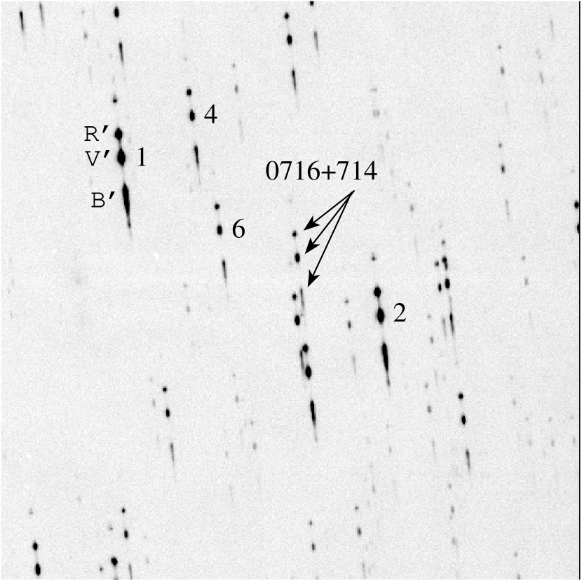
Figure 1: An example frame taken with the novel photometric system. Labeled are target blazar and four reference stars used for flux calibration. The $B^{\prime}$, $V^{\prime}$, and $R^{\prime}$ “images” are marked for Star 1 for an example. North is to the up and east, to the left.

An example frame is shown in Figure 1. We rotated the objective prism (and thus the dispersion direction) by a small angle from the standard vertical position. As the result, some overlaps of images were resolved, especially the potential overlap of the $B^{\prime}$ image of S5 0716+714 with the $R^{\prime}$ image of a star below (for a comparison, see Fig. 1 in this paper and Fig. 2 of Wu et al., 2007a).

The data reduction included bias subtraction, flat-fielding, extraction of instrumental aperture magnitude, and flux calibration. We defined a specially shaped aperture, as in Wu et al. (2007a), but with an update. In Wu et al. (2007a), the traditional circular aperture was equally split into two semicircles and a rectangle was inserted between them. Then an elongated aperture was obtained for the elongated images. For the inclined and elongated stellar images in this paper, we replaced the rectangle with a parallelogram. The chords of the two semicircles were attached to the top and bottom sides of the parallelogram, respectively, while the left and right sides of the parallelogram were set parallel to the dispersion line. Different parallelogram heights were adopted for the apertures in different passbands. They are 11, 7, and 4 pixels for the $B^{\prime}$, $V^{\prime}$, and $R^{\prime}$ images, respectively. The corresponding parallelogram widths (or the diameters of the semicircles) were set to be 5, 6, and 6 pixels, respectively. All sky annuli were set to have inner and outer radii of 11 and 15 pixels, but an area within 6 pixels in right ascension to the central axis of the aperture was excluded in order to eliminate the possible contamination of the background by the apertures. Stars 1, 2, and 4 in Villata et al. (1998) were used as reference stars. Their average brightness was utilized to calibrate the flux of S5 0716+714. Star 6 is slightly brighter than S5 0716+714 and was used as a check star (for a reasonable selection of reference and check stars, see Howell et al., 1988). The above aperture sizes in the three bands were chosen based on several trials to minimize the scatters in the differential magnitudes between the check star and the three reference stars. As in Wu et al. (2007a), the standard $B^{\prime}$, $V^{\prime}$, and $R^{\prime}$ magnitudes of these four stars were mimicked by their broadband $B$, $V$, and $R$ magnitudes. There should be some differences between these two magnitude systems, but they are tiny (Wu et al., 2007a), and are irrelevant for the results of our variability study presented here. The results are presented in Table 1. The columns are observation date and time (UT), Julian Date, exposure time, and magnitudes and errors of S5 0716+714 and differential magnitudes of star 6 in the $B^{\prime}$, $V^{\prime}$, and $R^{\prime}$ bands, respectively.

3 RESULTS

3.1 Light Curves

Figure 2 shows the total light curves of S5 0716+714 in the $B^{\prime}$, $V^{\prime}$, and $R^{\prime}$ bands. The $B^{\prime}$ and $R^{\prime}$ band light curves are shifted by 0.2 and $-0.5$ magnitudes, respectively, in order to make the variations clearly visible. The nightly-averaged brightness of this object was quite stable in this period and varies by less than 0.2 mags. On the other hand, intranight variations can still be observed on most nights by visual inspection.

We then performed a quantitative assessment on whether there are variations on these seven nights. Here we used the one-way analysis of variance (ANOVA) proposed by de Diego et al. (1998) and de Diego (2010). It is proved to be a powerful and robust estimator for variations (de Diego, 2010). In brief, the observations on each night were divided into groups of five consecutive data points. The variance of the means of each group about the overall mean was computed, as was the mean of the variances or dispersions (residuals) within each group. Then the ratio between these two variances was calculated and multiplied by five, the number of observations in each group. The value obtained behaves as the $F$ statistic. For a certain significance level, if $F$ exceeds the critical value, the null hypothesis that there is no variation will be rejected. The results are presented in Table 2. Column 1 is the Julian Date. Columns 2 and 3 are the degrees of freedom for the groups and residuals, respectively. Columns 4, 5, and 6 are $F$ values in the $B^{\prime}$, $V^{\prime}$, and $R^{\prime}$ bands, respectively. Column 7 is the critical value at the 99% significance level at the specified two degrees of freedom of Columns 2 and 3. Column 8 indicates whether there is variation. As can be seen, there are variations on JDs 2,454,088, 2,454,090, 2,454,092, and 2,454,097. The $F_{\rm B^{\prime}}$, $F_{\rm V^{\prime}}$, and $F_{\rm R^{\prime}}$ are all greater than the critical values on the four nights. On one more night, JD 2,454,091, there may be variation, too. The $F_{\rm V^{\prime}}$ and $F_{\rm R^{\prime}}$ are greater than the critical value, whereas the $F_{\rm B^{\prime}}$ is slightly smaller than it on that night. On the two remaining nights, JDs 2,454,093 and 2,454,094, there is no variation.

Figures 3, 4, 5, and 6 show the intranight light curves of S5 0716+714 on the four nights with variations, JDs 2,454,088, 2,454,090, 2,454,092, and 2,454,097, respectively. The associated small panels give the differential light curves of the check star (the means were set to 0). For these four nights, we calculated the intranight variation amplitudes with the definition of Heidt & Wagner (1996), $A=\sqrt{(m_{\rm max}-m_{\rm min})^{2}-2\sigma^{2}}$, where $m_{\rm max}$ and ${m_{\rm min}}$ are the faintest and brightest magnitudes during any given night, respectively and $\sigma$ is the standard deviation of the ’variation’ of the check star. The last point in the $R^{\prime}$-band light curve on JD 2,454,088 and the point at (0.26764, 14.034) in the $B^{\prime}$-band light curve on JD 2,454,097 are likely to be spurious measurements (see Figs. 3 and 6) and were discarded before the calculations. The results are listed in Table 3. It can be seen that the $B^{\prime}$-band variations have the largest amplitudes and the $V^{\prime}$- and $R^{\prime}$-band amplitudes are similar, with the latter lightly larger than the former on three of the four nights. In the shock-in-jet model, the variation amplitude decreases towards longer wavelengths. This has been observed in S5 0716+714 (e.g., Wu et al., 2007a; Poon et al., 2009; Fan et al., 2009) and in other blazars (e.g., Nesci et al., 1998; Fan & Lin, 2000; Dai et al., 2011). However, the amplitudes may also be related to the relative position of the frequency at which the observations were made and the peak frequency of the synchrotron component in the SED of blazars. The latter frequency itself may also shift from time to time (e.g., Giommi et al., 1999, 2000; Tavecchio et al., 2001; Zhang et al., 2010b). Taking these facts into account, our results that the $R^{\prime}$-band amplitudes are slightly larger than the $V^{\prime}$-band ones may not be unreasonable. As mentioned in Wu et al. (2007a) and Dai et al. (2011), the larger variation amplitude at higher frequency can partly explain the BWB chromatism observed in blazars.

3.2 Color-Magnitude Correlation

Controversy exists in the studies of the spectral or color behavior of blazars, as mentioned in §1. For our data on the four nights with variations, JDs 2,454,088, 2,454,090, 2,454,092, and 2,454,097, the color indices $B^{\prime}-V^{\prime}$ and $B^{\prime}-R^{\prime}$ were calculated and plotted against the $B^{\prime}$ magnitudes in the left and right panels of Figure 7, respectively. Different symbols mark data on different nights. They were fitted linearly and separately for each single night. We used the BCES regression (bivariate correlated errors and intrinsic scatters, Akritas & Bershady, 1996) to do the fitting. The BCES regression has the advantage of taking into consideration not only the measurement errors, but also the intrinsic scatters. The regression lines are plotted in Figure 7 with different styles for different nights. The thick solid lines are the fittings to all points. The correlation coefficients are given at the upper-left corners. It can be seen that the object shows strong BWB chromatisms on both intranight and internight timescales. This result is in agreement with several previous results (Wu et al., 2005, 2007a; Hao et al., 2010; Chandra et al., 2011) and with the short-term behavior obtained by Ghisellini et al. (1997) and Zhang et al. (2008). The much larger correlation coefficient in the right panel indicates a stronger correlation between $B^{\prime}-R^{\prime}$ and $B^{\prime}$ than between $B^{\prime}-V^{\prime}$ and $B^{\prime}$. A similar result has been reported by Raiteri et al. (2003), who found a stronger BWB trends with the $B-I$ color than with the $B-R$ color.

In addition to the flatter-when-brighter trend during rapid flares, Ghisellini et al. (1997) have reported that the correlation was rather insensitive for the long-term variations of S5 0716+714. A similar phenomenon was also recognized by Raiteri et al. (2003) in the same object. Our monitoring lasted for only ten days, so we cannot address the long-term color behavior of this object.

3.3 Color Evolution During Flares

In a variety of blazar emission models, one expects an interplay between gradual particle acceleration, radiative cooling and escape. This will lead to a loop-like path of the blazar’s state in a color-magnitude (or spectral index-flux) diagram. The direction of this spectral hysteresis can be either clockwise or anticlockwise, depending on the relative values of the acceleration, cooling and escape timescales (Chiaberge & Ghisellini, 1999; Dermer, 1998), as well as the frequency at which the observation is made relative to the peak frequency of the synchrotron component in the SED of the blazar (see Figs. 3 and 4 in Kirk et al., 1998). The loop path has been frequently reported in X-rays (e.g., Sembay et al., 1993; Takahashi et al., 1996; Kataoka et al., 1999; Zhang et al., 1999, 2002; Malizia et al., 2000; Ravasio et al., 2004) and, in one case, in the infrared (Gear et al., 1986). In the optical regime, Xilouris et al. (2006) have reported a similar pattern, and Wu et al. (2007a) showed a clockwise loop with the nightly means of magnitudes and colors. Such hysteresis behavior will inevitably translate into inter-band time lags.

In our monitoring, there are some mini-flares. The one with the largest amplitude occurred from 0.245 to 0.292 on JDs 2,454,088 (see Fig. 3). We checked the color evolution during that flare. Figure 8 displays the result. The numbers associated with the points signify the evolutionary sequence, with the beginning and end points marked by the filled circle and square, respectively. There is a hint of a clockwise loop when we check only the points, but the relatively large errors prevent us from drawing a convincing conclusion. Therefore, in order to observe an optical hysteresis loop on the color-magnitude diagram, more accurate observations are needed, preferentially during a flare with a larger amplitude than that of the current one. High temporal resolution may also be crucial.

3.4 Cross Correlation Analyses and Time Lags

We then performed the inter-band correlation analyses and searched for the possible inter-band time delay. These are carried out on the intranight light curves for the four nights with variations, JDs 2,454,088, 2,454,090, 2,454,092 and 2,454,097.

We at first used the z-transformed discrete correlation functions (ZDCFs; Alexander, 1997) to search for the $B^{\prime}$–$V^{\prime}$, $V^{\prime}$–$R^{\prime}$, and $B^{\prime}$–$R^{\prime}$ correlations. The ZDCF differs from the discrete correlation function (DCF) of Edelson & Krolik (1988) in that it bins the data points into equal population bins and uses Fisher’s z-transform to stabilize the highly skewed distribution of the correlation coefficient. It is much more efficient than the DCF in uncovering correlations involving the variability timescale, and deals with under-sampled light curves better than both the DCF and the interpolated cross-correlation function (ICCF; Gaskell & Peterson, 1987). For each correlation, a Gaussian fitting (GF) was made to the central ZDCF points with ZDCF value greater than $\sim 75\%$ of the peak value. The time where the Gaussian profile peaks denotes the lag between the correlated light curves.

The results are listed in Table 4 and displayed in Figures 9, 10, 11, and 12 for JDs 2,454,088, 2,454,090, 2,454,092, and 2,454,097, respectively. In each panel, Julian Date and the correlated passbands ($B^{\prime}$–$V^{\prime}$, $V^{\prime}$–$R^{\prime}$, or $B^{\prime}$–$R^{\prime}$) are given at the upper-left corner. The peak of the Gaussian profile (the dashed line) is marked with a vertical dotted line. The corresponding lag is given at the upper-right corner. A positive lag means that the former variation leads the latter one.

One problem in the GF is that it usually gives an unreliable and under-estimated error for the lag due at least to the statistically non-independent ZDCF points. Then, although the lags obtained from the ZDCF+GF method generally have significance greater than $3\sigma$, they should be taken with caution.

Another way to measure the lags and their errors is the ICCF (Gaskell & Peterson, 1987). The error was estimated with a model-independent Monte Carlo method, and the lag was taken as the centroid of the cross-correlation functions that were obtained with a large number of independent Monte Carlo realizations. This is the flux-randomization/random-subset-selection (FR/RSS) approach, as described by Peterson et al. (1998) and Peterson et al. (2004). In the current work, five thousand independent Monte Carlo realizations were performed on the light curves on JDs 2,454,088, 2,454,090, 2,454,092, and 2,454,097, and the lags and errors were obtained and are presented in Table 4. One can see from the table that although the ZDCF+GF and FR/RSS lags are usually consistent with each other, the FR/RSS errors are much larger than the corresponding ZDCF+GF errors. The FR/RSS lags have significance lower than $3\sigma$ except for the $V^{\prime}-R^{\prime}$ and $B^{\prime}-R^{\prime}$ lags on JD 2,454,090. On that night, the variability at the $B^{\prime}$ and $V^{\prime}$ bands lead that at the $R^{\prime}$ band by about 30 minutes.

A few optical lags have been reported in several blazars before. For example, Romero et al. (2000) derived a $\sim 4$ minute lag of the $R$ band variations relative to the $V$ band variations for PKS 0537-441 (see their Fig. 5). BL Lac was observed to have its $I$ band variations delayed by $\sim 0.2$ hours with respect to its $B$ band variations (Papadakis et al., 2003). The same authors also reported a lag of $0.9\pm 1.0$ hours of the $I$ band variations relative to the $B$ band variations for S4 0954+658 (Papadakis et al., 2004). For S5 0716+714, Qian et al. (2000) found an upper limit of 6 minutes for the time lag between the $V$ and $I$ band variations. Similarly, Villata et al. (2000) reported an upper limit of 10 minutes on the delay of the $I$ band variations relative to the $B$ band variations. Stalin et al. (2006) also presented time lags of 6 and 13 minutes for the $V$ and $R$ variations on two nights. But they also cautioned about the low significance level of their results. Most recently, Poon et al. (2009) found a possible lag of about 11 minutes between $B$ and $I$ band variations, and Zhang et al. (2010a) reported possible lags of a few minutes between low and high optical frequencies. These previous lags are either upper limits or cautioned by the authors to have low confidence levels. In the current work, however, the variability at short wavelengths were observed to lead that at long wavelengths on at least one night. This positive detection of inter-band time delays presumably has taken advantage of the simultaneous measurements at three optical wavelengths of our novel photometric system.

4 CONCLUSIONS AND DISCUSSIONS

4.1 Conclusions

We monitored S5 0716+714 for 7 nights with our novel photometric system in 2006 December. The photometry was carried out simultaneously at three optical wavelengths. The object did not show large-amplitude internight variations during this period, but displayed intranight variations on four nights and probable variations on one more. Strong BWB chromatism was detected on both intranight and internight timescales. For the four nights with variations, the intranight variation amplitude decreases in the wavelength sequence of $B^{\prime}$, $R^{\prime}$, and $V^{\prime}$. Cross correlation analyses revealed that the variations at the $B^{\prime}$ and $V^{\prime}$ bands led that at the $R^{\prime}$ band by about 30 minutes on one night.

4.2 Discussion on Color Behavior

S5 0716+714 showed a strong BWB chromatism during this period, either when the data are considered together or separately for individual nights. Despite the strong correlation, the points are in fact quite diffuse on the color-magnitude map (Fig. 7). Data on different nights occupy quite different regions, and follow distinct color-magnitude correlations. This dispersion is also evident in Wu et al. (2007a) (their Fig. 9). As mentioned in that paper and Dai et al. (2011), differences in variation amplitudes and paces (the lag) can both lead to the observed BWB chromatism. The variation amplitudes and the possible lags presented in this paper vary from night to night. So the dispersion on the color-magnitude map may be linked to the dispersion on the intranight variation amplitudes and/or the possible lags.

For the spectral or color behavior of blazars, different authors have drawn different conclusions. However, their results on the color-magnitude correlation of blazars may be biased by many aspects. Here we discuss some of them.

1. Non-simultaneous measurements at different wavelengths. Strictly speaking, the spectral or color index should be calculated with simultaneously measured fluxes or magnitudes at different wavelengths. However, most observations can only obtain quasi-simultaneous measurements. For blazars which do not show significant variations on very short timescales ($\lesssim 0.5$ hour), this may not be a problem. However, for those showing very fast variations, like S5 0716+714, as mentioned in the first section, this may be a serious problem. The intrinsic brightness of the object may change measurably when two observations are made successively at separated wavelengths. These two observations will result in a wrong spectral or color index. Although an interpolation can ameliorate this problem to some extent, the irregularity of the variability of blazars makes the interpolation usually unpractical. Our novel photometric system with the MPIF has the ability to take measurements simultaneously at three wavelengths. It can thus trace color changes accurately.

2. Observations taken at multiple telescopes and/or sites. There are likely systematic differences between data obtained with different telescopes. The difference can be 0.05 mag or even higher (e.g., Ghisellini et al., 1997). Then the color index will have an error close to 0.07–0.1 mag, a value comparable to the scale of the color change. This error will definitely weaken the color-magnitude correlation.

3. Inclusion of other components of variation. In addition to the shock-in-jet component, other mechanisms may be involved and dominant for an episode in blazar variability, such as the geometric effects suggested for S4 0954+658 (Wagner et al., 1993) and for S5 0716+714 (Wu et al., 2005). These effects lead to achromatic variations. In another BL Lac object, OJ 287, a huge achromatic outburst during 1994-96 was reported by Sillanpää et al. (1996). However, this outburst was dominated by a component presumably resulting from the interaction of the primary accretion disk and the secondary black hole in a binary black hole system (Lehto & Valtonen, 1996; Valtaoja et al., 2000; Liu & Wu, 2002; Valtonen et al., 2008). When the blazar variability was isolated, it showed a BWB trend (Wu et al., 2006).

4. Utilization of the averaged fluxes. If, for a blazar, the difference between variation amplitudes at different wavelengths is very small, and the spectral change is mainly resulting from time lag, we will not derive a spectral change when averaging the fluxes within a timescale far longer than the time lag. Therefore, it is not surprising that Sagar et al. (1999) and Stalin et al. (2006) claimed no spectral change, because they used the averaged flux or magnitude to derive the spectral or color index. However, when the amplitude difference in a blazar dominates the color change, the color change may also be detected by using averaged fluxes.

5. Utilization of closely separated frequencies. The $B-V$ and $V-R$ color indices change much less than the $B-R$, $V-I$, and $B-I$ color indices do. This has been illustrated by Raiteri et al. (2003) and this work.

There may be other barriers for the detection of the color or spectral changes and the color-magnitude correlations. These are the five major issues. Some of them may combine to function in the observations. For example, a campaign involving several telescopes usually suffer from the first two, as in the case of Ghisellini et al. (1997) and Raiteri et al. (2003).

Our photometric system has the advantage of simultaneous measurements at three optical wavelengths, and suffers none of the above 5 barriers in the detection of the color change. So the resulting color behavior should have higher confidence level than those from previous non- or quasi-simultaneous observations.

4.3 Discussion on Time Lag

A few intrinsic or extrinsic models have been proposed to explain the variability of blazars. The most popular is the shock-in-jet or internal shock model, in which shocks propagate down the relativistic jet, accelerating particles and/or compressing magnetic fields, leading to the observed variability. Depending on the balance between escape, acceleration, and cooling of the electrons with different energy, either soft (low energy) or hard (high energy) lags are expected (e.g., Kirk et al., 1998; Sokolov et al., 2004; Marscher, 2006). In fact, time lags between variations at much separated wavelengths are well known. For example, the soft X-ray variations were observed to lag the hard X-rays by about 1 hour in Mrk 421 (Takahashi et al., 1996) and by about 1000 s in S5 0716+714 (Zhang et al., 2010b). In PKS 2155-304, the X-ray flare appears to lead the EUV and UV fluxes by 1 and 2 days, respectively (Urry et al., 1997). Sometimes, the lags may show as the offsets between the X-ray knots and the radio or optical ones in the relativistic jets of radio galaxies, with the X-ray knots being closer to the core (e.g. Bai & Lee, 2003).

In optical regime, several authors claimed no detection of inter-band delays (e.g. Hao et al., 2010; Carini et al., 2011). Some other claimed the opposite, as mentioned in §3.4. Four key parameters probably determine whether the optical time lags can be detected: (1) wavelength separation, (2) variation amplitude, (3) temporal resolution, and (4) measurement accuracy. For the first factor, the larger the wavelength separation, the easier the lag will be detected. Then a $B-R$ or $B-I$ correlation should be performed rather than a $B-V$ or $V-R$ correlation. For the second, blazars with high duty cycles and large variation amplitudes should be observed for the search of the lag. For the third, a temporal resolution of less than 5 minutes is favorable, because most reported time lags are less than 10 minutes, as mentioned above. For the fourth, bright sources should be monitored. S5 0716+714 is one of the brightest blazars in the optical regime. It shows a high variation rate and has a high duty cycle, as mentioned in §1. This makes it probably the best candidate to be monitored for the search of the optical lags.

Our photometric system has the advantage of simultaneous measurements at multiple wavelengths and increases the temporal resolution significantly in each single wavelengths. With this system, we detected the time delays on one night. On the other and, our photometric system has its own deficiencies. For example, because of the elongated stellar images on the CCD frames, it is hard to accurately define the center of the aperture, especially for the $B^{\prime}$-band images. This results in an extra error in the data reduction. Another drawback may be that the wavelength separation between the $B^{\prime}$ and $R^{\prime}$ bands is not large enough. Therefore, a photometric system with a light splitting device may be more suitable in searching for the optical lags. When achieving a temporal resolution of about or higher than 1 minute, which is more than an order of magnitude shorter than the timescale of the optical variability of S5 0716+714 (Sasada et al., 2008; Rani et al., 2010a; Chandra et al., 2011), the traditional quasi-simultaneous photometric system may also be able to detect the optical lags with high confidence level.

Figure 2: Light curves in $B^{\prime}$, $V^{\prime}$, and $R^{\prime}$ bands for the entire monitoring period. For clarity, the $B^{\prime}$ and $R^{\prime}$ band light curves are shifted by 0.2 and $-0.5$ magnitudes, respectively.

Figure 3: Intranight light curves on JD 2,454,088 in the $B^{\prime}$, $V^{\prime}$, and $R^{\prime}$ bands. The associated small panels give the differential light curves of the check star (star 6).

Figure 4: Intranight light curves on JD 2,454,090 in the $B^{\prime}$, $V^{\prime}$, and $R^{\prime}$ bands. The associated small panels give the differential light curves of the check star (star 6).

Figure 5: Intranight light curves on JD 2,454,092 in the $B^{\prime}$, $V^{\prime}$, and $R^{\prime}$ bands. The associated small panels give the differential light curves of the check star (star 6).

Figure 6: Intranight light curves on JD 2,454,097 in the $B^{\prime}$, $V^{\prime}$, and $R^{\prime}$ bands. The associated small panels give the differential light curves of the check star (star 6).

Figure 7: Color-magnitude diagrams for JDs  2,454,088, 2,454,090, 2,454,092, and 2,454,097. The left panel is for $B^{\prime}-V^{\prime}$ color, while the right is for $B^{\prime}-R^{\prime}$ color. Different symbols represent data on different nights. They are fitted linearly and separately for each individual night and are shown with different lines. The solid lines are fittings to all points, with the corresponding correlation coefficients given at the upper-left corners. The errors are not plotted here for clarity. The mean magnitude error is 0.018 mags and the mean color error is 0.022 mags.

Figure 8: Color evolution during flares from 0.245 to 0.292 on JDs 2,454,088. The filled circle and square mark the beginning and ending points, respectively. The numbers indicate the points in time sequence.

Figure 9: ZDCF correlation and fitting results on JD 2,454,088. The dashed lines are Gaussian fittings to the points, and their peaks are marked with the vertical dotted lines.

Figure 10: ZDCF correlation and fitting results on JD 2,454,090. The dashed lines are Gaussian fittings to the points, and their peaks are marked with the vertical dotted lines.

Figure 11: ZDCF correlation and fitting results on JD 2,454,092. The dashed lines are Gaussian fittings to the points, and their peaks are marked with the vertical dotted lines.

Figure 12: ZDCF correlation and fitting results on JD 2,454,097. The dashed lines are Gaussian fittings to the points, and their peaks are marked with the vertical dotted lines.

Table 1: Observational Log and Results in the $B^{\prime}$, $V^{\prime}$ and $R^{\prime}$ Bands

Date	Time	Julian Date	Exp.	$B^{\prime}$	$B^{\prime}_{\rm err}$	$\delta B^{\prime}$	$V^{\prime}$	$V^{\prime}_{\rm err}$	$\delta V^{\prime}$	$R^{\prime}$	$R^{\prime}_{\rm err}$	$\delta R^{\prime}$
(1)	(2)	(3)	(4)	(5)	(6)	(7)	(8)	(9)	(10)	(11)	(12)	(13)
2006 12 18	16:03:37.0	2454088.16918	150	14.340	0.018	$-$0.014	13.745	0.011	0.008	13.263	0.017	0.014
2006 12 18	16:06:25.0	2454088.17112	150	14.298	0.017	$-$0.000	13.740	0.011	$-$0.021	13.271	0.017	$-$0.015
2006 12 18	16:09:14.0	2454088.17308	150	14.325	0.018	$-$0.025	13.751	0.012	$-$0.011	13.293	0.017	$-$0.005
2006 12 18	16:12:02.0	2454088.17502	150	14.320	0.017	$-$0.004	13.738	0.011	$-$0.009	13.292	0.017	$-$0.010
2006 12 18	16:14:51.0	2454088.17698	150	14.316	0.017	0.011	13.771	0.011	$-$0.011	13.279	0.017	$-$0.001

Note. — Table 1 is published in its entirety in the electronic edition of the Astronomical Journal. A portion is shown here for guidance regarding its form and content.

Table 2: Variation Test Result

JD	$\nu_{1}$	$\nu_{2}$	$F_{\rm B^{\prime}}$	$F_{\rm V^{\prime}}$	$F_{\rm R^{\prime}}$	$F_{0.01}$	Var?
2,454,088	26	108	23.705	29.534	25.166	1.930	Y
2,454,090	36	148	4.233	16.408	3.600	1.763	Y
2,454,091	37	152	1.599	5.270	2.817	1.750	Y?
2,454,092	36	148	8.342	13.132	8.296	1.763	Y
2,454,093	38	156	0.687	2.584	1.317	1.740	N
2,454,094	13	56	0.684	0.523	1.521	2.465	N
2,454,097	38	156	4.359	11.649	3.068	1.740	Y

Table 3: Intranight Variation Amplitude

	$A_{\rm B^{\prime}}$	$A_{\rm V^{\prime}}$	$A_{\rm R^{\prime}}$
JD	(mag)	(mag)	(mag)
2,454,088	0.262	0.222	0.233
2,454,090	0.208	0.148	0.152
2,454,092	0.182	0.132	0.172
2,454,097	0.206	0.134	0.110

Table 4: Time Lags Between Different Wavelengths

	$B^{\prime}$–$V^{\prime}$			$V^{\prime}$–$R^{\prime}$			$B^{\prime}$–$R^{\prime}$
JD	ZDCF+GF	FR/RSS		ZDCF+GF	FR/RSS		ZDCF+GF	FR/RSS
2,454,088	1.16$\pm$0.08	1.26$\pm$1.92		0.77$\pm$0.08	0.09$\pm$2.04		2.16$\pm$0.08	2.40$\pm$2.16
2,454,090	5.48$\pm$0.51	4.98$\pm$5.82		25.35$\pm$0.81	28.14$\pm$7.02		26.46$\pm$0.92	30.12$\pm$11.04
2,454,092	2.64$\pm$0.37	2.52$\pm$3.48		1.54$\pm$0.40	3.30$\pm$2.94		4.89$\pm$0.46	6.78$\pm$4.26
2,454,097	$-$9.76$\pm$0.47	$-$10.2$\pm$4.38		4.60$\pm$0.40	3.54$\pm$5.76		$-$0.68$\pm$0.56	$-$4.86$\pm$9.66

References

- Akritas & Bershady (1996) Akritas, M. G. & Bershady, M. A., 1996, ApJ, 470, 706
- Alexander (1997) Alexander, T. 1997, in Astronomical Time Series, ed. D. Maoz, A. Sternberg, & E. M. Leibowitz (Dordrecht: Kluwer), 163
- Anderhub et al. (2009) Anderhub, H., et al. 2009, ApJ, 704, L129
- Bai & Lee (2003) Bai, J. M., & Lee, M. G., 2003, ApJ, 585, L113
- Böttcher (2007) Böttcher, M., 2007, ApS&S, 309, 95
- Böttcher et al. (2007) Böttcher, M., et al. 2007, ApJ, 670, 968
- Böttcher et al. (2009) Böttcher, M., et al. 2009, ApJ, 694, 174
- Carini et al. (2011) Carini, M. T., Walters, R., & Hopper, L. 2011, AJ, 141, 49
- Chandra et al. (2011) Chandra, S., Baliyan, K. S., Ganesh, S., & Joshi, U. C., 2011, ApJ, 731, 118
- Chen et al. (2008) Chen, A. W., et al. 2008, A&A, 489, L37
- Chiaberge & Ghisellini (1999) Chiaberge, M., & Ghisellini, G. 1999, MNRAS, 306, 551
- Dai et al. (2011) Dai, Y., Wu, J., Zhu, Z., Zhou, X., & Ma, J. 2011, AJ, 141, 65
- de Diego (2010) de Diego, J. A., 2010, AJ, 139, 1269
- de Diego et al. (1998) de Diego, J. A., Dultzin-Hacyan, D., Ramírez, A., & Benítez, E., 1998, ApJ, 500, 69
- Dermer (1998) Dermer, C. D., 1999, ApJ, 501, L157
- Edelson & Krolik (1988) Edelson, R. A., & Krolik, J. H., 1988, ApJ, 333, 646
- Fan & Lin (2000) Fan, J. & Lin, R. 2000, ApJ, 537, 101
- Fan et al. (2009) Fan, J., Peng, Q. S., Tao, J., Qian, B. C., & Shen, Z. Q. 2009, AJ, 138, 1428
- Fan et al. (2011) Fan, J., Tao, J., Qian, B., Liu, Y., Yang, J., Pi, F., & Xu, W., 2011, RAA, 11, 1311
- Ferrero et al. (2006) Ferrero, E., Wagner, S. J., Emmanoulopoulos, D., & Ostorero, L. 2009, A&A, 457, 133
- Foschini et al. (2006) Foschini, L., et al. 2006, A&A, 455, 871
- Gaskell & Peterson (1987) Gaskell, C. M. & Peterson, B. M., 1987, ApJS, 65, 1
- Gear et al. (1986) Gear, W. K., Robson, E. I., & Brown, L. M. J. 1986, Nature, 324, 546
- Ghisellini et al. (1997) Ghisellini, G., et al. 1997, A&A, 327, 61
- Giommi et al. (1999) Giommi, P., et al. 1999, A&A, 351, 59
- Giommi et al. (2008) Giommi, P., et al. 2008, A&A, 487, L49
- Giommi et al. (2000) Giommi, P., Padovani, P., & Perlman, E. 2000, MNRAS, 317, 743
- Gu et al. (2006) Gu, M. F., Lee, C.-U., Pak, S., Yim, H. S., & Fletcher, A. B. 2006, A&A, 450, 39
- Gu & Ai (2011) Gu, M. F. & Ai, Y. L. 2011, A&A, 528, 95
- Gupta et al. (2008) Gupta, A., et al. 2008, AJ, 135, 1384
- Hao et al. (2010) Hao, J., Wang, B., Jiang, Z., & Dai, B. 2010, RAA, 10, 125
- Howell et al. (1988) Howell, S. B., Mitchell, K. J., & Warnock, A. 1998, AJ, 95, 247
- Hu et al. (2006) Hu, S., Zhao, G., Guo, H. Y., Zhang, X., & Zheng, Y. G. 2006, MNRAS, 371, 1243
- Heidt & Wagner (1996) Heidt, J. & Wagner, S. J. 1996, A&A, 305, 42
- Kataoka et al. (1999) Kataoka, J., et al. 1999, ApJ, 528, 243
- Kirk et al. (1998) Kirk, J. G., Rieger, F. M., & Mastichiadis, A. 1998, A&A, 333, 452
- Lehto & Valtonen (1996) Lehto, H. J. & Valtonen, M. J. 1996, ApJ, 460, 207
- Lin et al. (1995) Lin, Y. C., et al. 1995, ApJ, 442, 96
- Liu & Wu (2002) Liu, F. K. & Wu, X. B. 2002, A&A, 388, L48
- Malizia et al. (2000) Malizia, A., et al. 2000, MNRAS, 312, 123
- Marscher (2006) Marscher, A. P. 2006, Chinese J. Astron. Astrophys., 6a, 262
- Montagni et al. (2006) Montagni, F., Maselli, A., Massaro, E., Nesci, R., Sclavi, S., & Maesano, M. 2006, A&A, 451, 435
- Nesci et al. (1998) Nesci, R., Maesano, M., Massaro, E., Montagni, F., Tosti, G., & Fiorucci, M. 1998, A&A, 332, L1
- Nesci et al. (2002) Nesci, R., Massaro, E., & Montagni, F. 2002, Publ. Astron. Soc. Aust. 19, 143
- Nesci et al. (2005) Nesci, R., Massaro, E., Rossi, C., Sclavi, S., Maesano, M., & Montagni, F. 2005, AJ, 130, 1466
- Nilsson et al. (2008) Nilsson, K., Pursimo, T., Sillanpää, A., Takalo, L. O., & Lindfors, E. 2008, A&A, 487, L29
- Ostorero et al. (2006) Ostorero, L., et al. 2006, A&A, 451, 797
- Papadakis et al. (2003) Papadakis, I. E., Boumis, P., Samaritakis, V. & Papamastorakis, J. 2003, A&A, 397, 565
- Papadakis et al. (2004) Papadakis, I. E., Samaritakis, V., Boumis, P., & Papamastorakis, J. 2004, A&A, 426, 437
- Peterson et al. (1998) Peterson, B. M., Wanders, I., Horne, K., Collier, S., Alexander, T., Kaspi, S., & Maoz, D. 1998, PASP, 110, 660
- Peterson et al. (2004) Peterson, B. M., et al. 2004, ApJ, 613, 682
- Pollock et al. (2007) Pollock, J. T., Webb, J, R., & Azarnia, G. 2007, AJ, 133, 487
- Poon et al. (2009) Poon, H., Fan, J. H., & Fu, J. N. 2009, ApJS, 185, 511
- Qian et al. (2000) Qian, B., Tao, J., & Fan, J. 2000, PASJ, 52, 1075
- Qian et al. (2002) Qian, B., Tao, J., & Fan, J. 2002, AJ, 123, 678
- Raiteri et al. (2003) Raiteri, C. M., et al. 2003, A&A, 402, 151
- Ramírez et al. (2004) Ramírez, A., de Diego, J. A., Dultzin-Hacyan, D., & González-Pérez, J. N. 2004, A&A, 421, 83
- Rani et al. (2010a) Rani, B., et al. 2010a, ApJ, 719, L153
- Rani et al. (2010b) Rani, B., et al. 2010b, MNRAS, 404, 1992
- Ravasio et al. (2004) Ravasio, M., Tagliaferri, G., Ghisellini, G., & Tavecchio, F. 2004, A&A, 424, 841
- Romero et al. (2000) Romero, G. E., Cellone, S. A., & Combi, J. A. 2000, AJ, 120, 1192
- Sagar et al. (1999) Sagar, R., Gopal-Krishna, Mohan, V., Pandey, A. K., Bhatt, B. C., & Wagner, S. J. 1999, A&AS, 134, 453
- Sasada et al. (2008) Sasada, M., et al. 2008, PASJ, 60, L37
- Sembay et al. (1993) Sembay, S., Warwick, R. S., Urry, C. M., Sokoloski, J., George, I. M., Makino, F., Ohashi, T., & Tashiro, M. 1993, ApJ, 404, 112
- Sillanpää et al. (1996) Sillanpää, A., et al. 1996, A&A, 315, L13
- Sokolov et al. (2004) Sokolov, A., Marscher, A. P., & McHardy, I. M. 2004, ApJ, 613, 725
- Stalin et al. (2009) Stalin, C. S., et al. 2009, MNRAS, 399, 1357
- Stalin et al. (2006) Stalin, C. S., Gopal-Krishna, Sagar, R., Wiita, P. J., Mohan, V., & Pandey, A. K. 2006, MNRAS, 366, 1337
- Tagliaferri et al. (2003) Tagliaferri, G., et al. 2003, A&A, 400, 477
- Takahashi et al. (1996) Takahashi, T., et al. 1996, ApJ, 470, L89
- Tavecchio et al. (2001) Tavecchio, F., et al. 2001, ApJ, 554, 725
- Urry et al. (1997) Urry, C. M., et al. 1997, ApJ, 486, 799
- Vagnetti et al. (2003) Vagnetti, F., Trevese, D., & Nesci, R. 2003, ApJ, 590, 123
- Valtaoja et al. (2000) Valtaoja, E., Teräsranta, H., Tornikoski, M., Sillanpää, A., Aller, M. F., Aller, H. D., & Hughes, P. A. 2000, ApJ, 531, 744
- Valtonen et al. (2008) Valtonen, M. J., et al. Nature, 452, 851
- Villata et al. (2000) Villata, M., et al. 2000, A&A, 363, 108
- Villata et al. (2008) Villata, M., et al. 2008, A&A, 481, L79
- Villata et al. (1998) Villata, M., Raiteri, C. M., Lanteri, L., Sobrito, G., & Cavallone, M. 1998, A&AS, 130, 305
- Wagner et al. (1993) Wagner, S. J., et al. 1993, A&A, 271, 344
- Wagner et al. (1996) Wagner, S. J., et al. 1996, AJ, 111, 2187
- Wagner & Witzel (1995) Wagner, S. J. & Witzel, A. 1995, ARA&A, 33, 163
- Wu et al. (2006) Wu, J., et al. 2006, AJ, 132, 1256
- Wu et al. (2005) Wu, J., Peng, B., Zhou, X., Ma, J., Jiang, Z., & Chen, J. 2005, AJ, 129, 1818
- Wu et al. (2007a) Wu, J., Zhou, X., Ma, J., Wu, Z., Jiang, Z., & Chen, J. 2007a, AJ, 133, 1599
- Wu et al. (2007b) Wu, J., Zhou, X., & Ma, J. 2007b, ASPC, 373, 199
- Xie et al. (2004) Xie, G. Z., Zhou, S. B., Li, K. H., Dai, H., Chen, L. E., & Ma, L. 2004, MNRAS, 348, 831
- Xilouris et al. (2006) Xilouris, E. M., et al. 2006, A&A, 448, 143
- Zhang et al. (2010a) Zhang, B., Dai, B., Zhang, L., Liu, J., & Cao, Z., 2010a, PASA, 27, 296
- Zhang et al. (2008) Zhang, X., et al. 2008, AJ, 136, 1846
- Zhang et al. (1999) Zhang, Y., et al. 1999, ApJ, 527, 719
- Zhang et al. (2002) Zhang, Y., et al. 2002, ApJ, 572, 762
- Zhang et al. (2010b) Zhang, Y., et al. 2010b, ApJ, 713, 180