A Few Lessons from pQCD Analysis at Low Energies

D.V. Shirkov

Abstract

Motivated by the recent 4-loop analysis of the JLab data on Bjorken Sum Rule, where the pQCD series seems to blow up at $\,|Q|\lesssim 1.5\,{\rm G}{\rm e\kern-1.07996ptV}\,,\,{\bar{\alpha}_{s}}\gtrsim 0.33\,,$ we overview the general origin of the divergency of common perturbation expansion over powers of a small coupling parameter in QFT and consider in detail the blowing-up phenomenon and accuracy of finite sums for simple alternating and non-alternating examples of divergent series.

1 Introduction

It is known since the mid-XX that the main computational tool of quantum theory, the perturbation expansion $\sum_{k}\alpha^{k}\,c_{k}(...)\,$ over powers of the small coupling parameter $\alpha$ , is not a convergent one; expansion coefficients grow factorially $c_{k}\sim k\,!\,.$ The reason is that every quantum amplitude (matrix element) $C(\alpha,...)$ is not a regular function of $\alpha$ at the origin $\alpha=0\,.$
Practically, the finite sum $\sum_{k}^{N}$ of such a series could blow up at $N\sim 1/\alpha\,.$
To illustrate, take a formal divergent series

$$f(g)\sim\sum_{n\geq 1}\,n!\,g^{n}\,=g+2\,g^{2}\,+\dots\,.$$ (1) Its finite sum $$f_{[k]}(g)=\sum_{n}^{k}\,f_{n};\quad f_{n}=n!\,g^{n}\,,$$ (2) according to the Poincaré estimate [1] can approximate an expanded function $\,F\,$ with accuracy $\Delta_{k}f(g)=f(g)-f_{[k]}(g)\sim f_{k}\,.$

Fig. 1 Values of $f_{k}$ terms at g=0.25.

Thus, the finite sum can provide us with the best possible accuracy  $[\Delta_{K}f(g)]_{opt}=f_{K}\,$ at an optimal number of terms

$$k=K\sim 1/g\,.$$ (3)

The very existence of this  lower limit of possible accuracy  is an exact antithesis to the case of convergence series : any attempt to increase the number of terms above $K$ leads to the lower accuracy. At  $g\lesssim 1\,$ this can happen for rather small $K\,$ values.

In the above formal example (1), at  g=0.25, with K=4, $\,f_{4}(0.25)=0.5625\,$ and $\,\Delta_{4}F(0.25)=f_{4}=3/32$ this lower limit of accuracy is about 16.7 % . For $\,f_{5}(0.25)=0.6798$, it is slightly worse – 17.2 %.

2 Divergent Series and their Summation

2.1 Explicit Illustrations

Consider the integral

$$A(g)=\tfrac{2}{\sqrt{\pi}}\int^{\infty}_{0}\,e^{-x^{2}-(g/4)\,x^{4}}\,dx\,;\quad g>0\,.$$ (4)

Expanding integrand in $g$ and changing the order of integration and summation one arrives at alternating divergent series

$$A(g)=\sum_{n\geq 0}\,(-g)^{n}\,A_{n}\,;\quad A_{n}=\frac{2}{4^{n}\sqrt{\pi}\,n\,!}\,\int\,e^{-x^{2}}\,x^{4n}\,dx\,;\quad A_{0}=1\,.$$ (5)

The $n\to\,\infty$ limit for $A_{n}$ coefficients can be estimated by the steepest descent method:

$$A_{n}^{as}\sim\int^{\infty}_{0}\,e^{n\,f(x)}\,dx\,,\quad f(x)=4\,\ln x-\frac{x^{2}}{n}\,;\quad\mbox{with result}\quad A_{k}^{as}=\frac{(k-1)\,!}{\sqrt{2\,\pi}}\,.$$

Here, the divergent series was obtained by formal manipulation with the finite expression. The finite sums $a_{[n]}(g)=g\,A_{1}-\dots\pm A_{n}\,(-g)^{n}\,$ of alternating series (5) can be compared with exact values of the function $A(g)=1-a(g)\,.$ For results of comparison see Fig.2. There, we show that starting from $g=0.25\,$ the $a_{[4]}$ curve passes farther from the exact one than the $a_{[3]}$ curve.

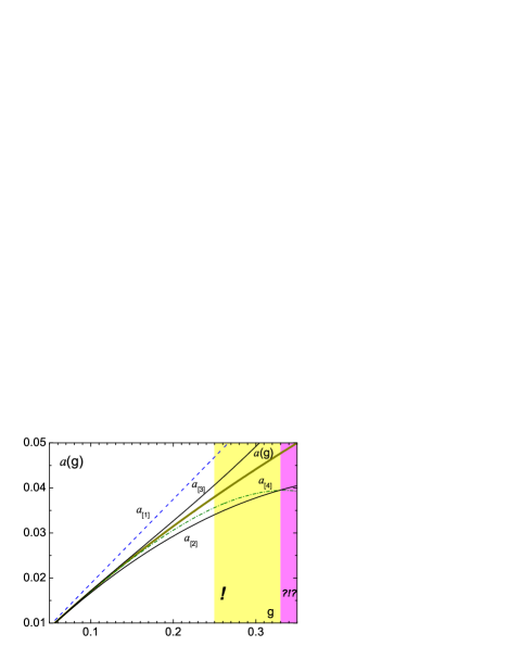
Figure 2: The $a_{[k]}$ approximants for the function $A(g)$. The mark of exclamation, “!” denotes the beginning of the yellow zone (= caution light) while the combination “?!?” marks the red zone.

A practical example of alternating divergent series gives the beta-function of the $g\varphi^{4}$ model. In the late 70s its expression

$$\beta_{\overline{\rm MS}}^{pt,4}(g)=\tfrac{3}{2}\,g^{2}-\tfrac{17}{6}g^{3}+16.27\,g^{4}-135.8\,g^{5}$$

known up to the $N^{3}LO$ term was used [2] as a starting point for the whole function $\,\beta_{\overline{\rm MS}}(g)\,$ restoration. In the reconstruction procedure (based also on asymptotic expression [4] for $\,\beta_{n}^{as}\,$) the Borel representation supplemented by conformal transformation was involved. The resulting closed formula

$$\beta_{\overline{\rm MS}}^{\scriptsize CB}(g)=\int^{\infty}_{0}\,\frac{dx}{g}e^{-x/g}\left(\frac{d}{dx}\right)^{5}\,x^{2}\,b_{3}(x)\,$$ (6)

can be used for next coefficient estimation. Later on, the next $N^{4}LO$ term was calculated [5, 6] $\beta_{5}=1420.6\,$ via Feynman diagrams. Comparing it with the prediction (6) $\beta_{5}^{CB}=1409.6\,$  gives the accuracy within 1 % !

Another model integral

$$C(g)=\tfrac{1}{\sqrt{\pi}}\int^{\infty}_{-\infty}\,e^{-x^{2}(1-\frac{\sqrt{g}}{4}\,x)^{2}}\,dx\to\sum_{k}g^{k}C_{k}\,;\quad C_{k}=A_{k}=\left.\tfrac{\Gamma(2k+1/2)}{4^{k}\,\Gamma(k+1)}\right|_{k\gg 1}\to\,\tfrac{\Gamma(k)}{\sqrt{2\,\pi}}\,$$ (7)

produces non-alternating asymptotic power series with the same coefficients. As far as this integral is also expressible in terms of Bessel functions (see Ref.[2], page 482), one has exact expression for the coefficients and can compare the finite sum approximations $c_{[n]}(g)=C_{1}+\dots+C_{n}\,g^{n}\,$ with exact values of $C(g)-1=c(g)\,$ – see Fig. 3.

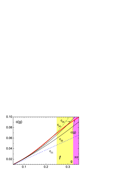
Figure 3: The $c_{[k]}$ approximants for the function $c(g)=C(g)-1\,.$

It is clear that the 2-term approximant (lower thin curve) is good up only to $g=0.15-0.20$ and the 3-term one (upper thin curve) up to $g\sim 0.33\,$ while the 4-term sum (upper broken curve) starts to deviate from $C(g)$ (red thick curve) at $g\sim 0.27\,!$

The model (7) is more instructive for our case motivated by the fresh signal from the perturbative Quantum Chromodynamics (pQCD) in the low-energy domain. There, the 4-loop analysis of rather precise JLab data on polarized Bjorken Sum Rule revealed [7] that the non-alternating series for the pQCD correction (eq.(3) in [7])

$$\Delta_{[4]}^{Bj}(\alpha_{s})=0.3183\,\alpha_{s}+0.3631\,\alpha_{s}^{2}+0.6520\,\alpha_{s}^{3}+1.804\,\alpha_{s}^{4}$$ (8)

does blow up at $\,\alpha_{s}\sim 0.35\,.$ It is noteworthy that the coefficient ratios here (1.1, 1.8, 2.8) are close to the factorial ones (1, 2, 3).

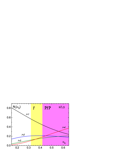
Figure 4: The $\alpha_{s}$ -dependence of the relative PT contributions to the Bjorken amplitude at the 4-loop level – based on Eq.(9).

Indeed, as it is shown on Fig.4, the 4-loop term ($\sim\alpha_{s}^{4}$) is close to the 3-loop one in the interval $0.3\lesssim\alpha_{s}\lesssim 0.4\,,$ while it approaches the 2-loop term at $\alpha_{s}\geq 0.4\,.$ We marked the first region as a “yellow zone”  and the second as a “red” one. Roughly, this corresponds to the rule $K\sim 1/\alpha_{s}\,,$ Eq.(3) with $K=i-1\,.$

Two other illustrations on Fig. 5 a,b, also taken from paper [7] demonstrate the lack of progress in the 4-loop description - marked by black hatching (SW-NE direction)- with respect to the 3-loop one (red hatching in the NW-SE direction).

Fig. 5a  The QCD perturbation analysis of the  Bjorken form-factor  confronted with JLab data in three- and four-loop orders.

Fig. 5b  Instability of the HT coefficient $\mu_{4}$ fitting of the Jlab data, as in Fig.5a

2.2 Asymptotic series and essential singularity

Turn to the origin of the non-convergent asymptotic series (AS) like in Eqs.(1),(6),(8). Usually, it is related with the essential singularity at the origin $\,\alpha=0\,$ that is a common property (in the theories of Big Systems) of the objects representable via Functional or Path Integral. This is the case for Turbulence, Classic and Quantum Statistics and Quantum Fields. Numerous examples are well known : the $\,\mathbf{e}^{-1/g}\,$ dependence of the energy gap in BCS and Bogoliubov theories of SuperConductivity : for tunneling probability in quantum mechanics. In the theory of Quantum fields (QFT) it was first discussed for QED by Dyson just 60 years ago [8] and soon after that implemented by Bogoliubov [9]; (for the QCD case, the same method was used in the so-called APT approach – see below Section 3).

Mathematically, the essential singularity origin is connected with the small parameter $g\,$ (or $\alpha$ ) attached to some nonlinear structure. In the quantum case, this is interaction term. Generally, a certain AS corresponds to a set of various functions. Hence, in physics,

The Asymptotic Series  “summation”  is an Art.

This motto really implies that for the adequate AS summation one should involve some additional arguments, like in the Eq. (6) example above.

2.3 Higher PT terms for   $\mathbf{e^{+}e^{-}\to}$ hadrons

As far as this meeting is devoted mainly to the electron-positron collider physics, turn to the inclusive $e^{+}e^{-}\to$ hadrons process. Two functions, the cross-section ratio $R(s)=1+r(s)\,,$ and the Adler function $D(Q^{2})=1+d(Q)\,$ are in use there. Table 1 presents the short summary of the PT terms relative contribution in the ‘moderate energy’  interval below $m_{\tau}\,.$

Table 1. Relative contributions  of 1-, …  4-loop terms in  $e^{+}e^{-}\to$  hadrons

Function	Scale/Gev	PT terms  (in %)
the loop number $\ell\ \to$		1	2	3	4
r(s)	1	65	19	55 ?!?	-39 ?!?
r(s)	1.78	73	13	24 ?!?	-10 ?!?
d(Q)	1	56	17	11 !	16 ?!?
d(Q)	1.78	75	14	6	5 !

In the upper two lines, for $r(s)\,,$ one can see the literally terrible effect of the $\pi^{2}$ terms on the higher $\ell=3,4\,$ contributions. This issue was resolved in the 80s[10, 11]. The net result is that in the annihilation channel, the s-channel, one should use some special QCD coupling ${\tilde{\alpha}}(s)\,$ instead of ${\bar{\alpha}_{s}}(Q^{2})\,.$ See below, eq.(9) and Fig.6a.

Concerning the higher contributions, $d_{\ell=3,4}\,,$ to the Adler function one observes the picture analogous to the one illustrated by Fig.4.

3 Analytic Perturbation Theory

3.1 A Few Words about APT

Analytic Perturbation Theory (APT) in QCD, is the closed theoretical scheme devised in the mid-90s [12] without Landau singularities and additional parameters. It stems from the imperatives of  RG-invariance, $Q^{2}$-analyticity, compatibility with linear integral (like, the Fourier) transformations and essentially incorporates non-perturbative $\,e^{-1/\alpha_{s}}$ (algebraic in $Q^{2}$) structures.

Instead of the power PT set $\,\bar{\alpha}_{s}(Q^{2})$,$\,\bar{\alpha}_{s}(Q^{2})$², $\,\bar{\alpha}_{s}(Q^{2})$${}^{3},\dots$ one has a non-power APT expansion set  {${\cal A}_{k}(Q^{2})$ } $k=1,2,\dots$ with all ${\cal A}_{k}(Q^{2})$ regular in the IR region. Accordingly, for the s-channel, there is another IR-regular set ${\tilde{\alpha}}_{k}(s)\,.$ The first functions ${\cal A}_{1}(Q^{2})=\alpha_{an}\,,$ and ${\tilde{\alpha}}_{1}(s)={\tilde{\alpha}}(s)$ at the one-loop case look rather simple

$$\alpha_{an}(Q^{2})=\frac{1}{\beta_{0}\,\ln(Q^{2}/\Lambda^{2})}+\frac{\Lambda^{2}}{\beta_{0}\,(\Lambda^{2}-Q^{2})}\,;\quad{\tilde{\alpha}}(s)=\frac{1}{\pi\,\beta_{0}}\,\arctan\frac{\pi}{\ln(Q^{2}/\Lambda^{2})}\,.$$ (9)

Both are presented on Fig.6a  together with common $\bar{\alpha}_{s}$ , singular at $Q=\Lambda=400\,{\rm M{\rm e\kern-1.19995ptV}}\,.$ Their regular LE behavior corresponds quantitatively to results of lattice simulation (see Fig.6b) down to $Q\sim 500\,{\rm M{\rm e\kern-1.19995ptV}}.$

Fig.6a  Analytic QCD couplings $\alpha_{an}(Q)$ and ${\tilde{\alpha}}(s)$ in comparison with common $\bar{\alpha}_{s}$ .

Fig.6b  The lattice $\alpha_{s}$ based on three-gluon vertex

As it can be seen from Fig.7 the APT+Higher Twist (HT) description of the JLab data looks quite satisfactory down to 350-400 MeV , that is to the $\Lambda_{QCD}$ scale !

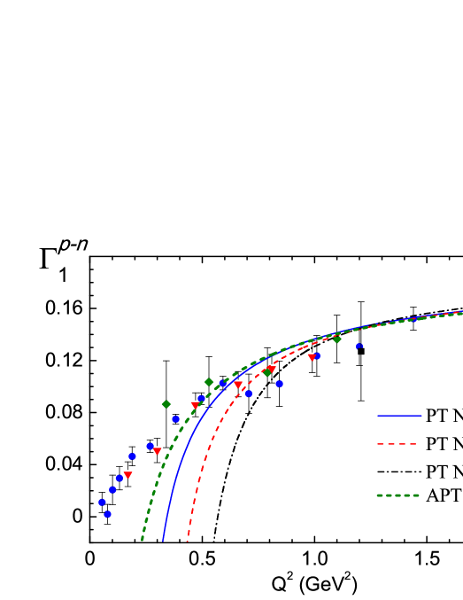
Figure 7: Reasonable fit of the JLab data by APT supplemented by Higher Twist (HT) terms (the upper green dotted curve) down to 350  MeV  . Three lower curves describe the standard PT fits.

We omit here technical details of the APT+HT analysis of paper [7]. Some of them can be seen in the last right columns of Table 2. There, higher PT and APT contributions to couple of sum rules are summarized.

Table 2.  Relative contributions (in %) of  1-,2-,3- and  4-loop  terms

Process		Scale/Gev	PT(in %)				APT ∗ aa
the loop number =			1	2	3	4	1	2	3
Bjorken SR	t	1	35	20	19 !	26 ?!?	80	19	1
Bjorken SR	t	1.78	56	21	13	11 !	80	19	1
GLS SumRule	t	1.78	65	24	11 !		75	21	4
Incl. $\tau$-decay	s	1.78	51	27	14	7 !	88	11	1

* The 4-loop APT contributions are negligible everywhere.

Invitation for Work (instead of Conclusion)

A number of topics is in order:

• Devising methods of AS summation, (including integral and conformal tricks),

• Devising Generating Function for HT terms in QCD

• either generalizing the minimal APT,

• Toy models for the 4-loop term predicting for other processes  $P_{i}$

• Set of analytic couplings $\,\alpha_{s}^{i}\,,$ each being adequate to a given process  $P_{i}$  ?

• Generating  HT  function for the each  $P_{i}$  ?

Acknowledgments

It is a pleasure to thank Dr. V. Khandramai for useful discussion and technical help. This research has partially been supported by the presidential grant Scient. School–3810.2010.2, RFFI grant 11-01-00182 and by the BelRFFR- JINR grant F10D-001.

References

- [1] H. Poincaré, Acta Mathematica, v.8, 205-344, (1886).
- [2] D.I.Kazakov and D.V.Shirkov, Fortsch.d.Physics 28, 465-489 (1980).
- [3] D.V.Shirkov, “Causality and Renorm Group” Lett.Math.Phys. v.1, 179-182 (1976).
- [4] L.N. Lipatov, Zh.Exp.Teor.Fiz v.72 411 (1977).
- [5] D.I. Kazakov, Phys.Lett. B133, pp.406-410 (1983).
- [6] K.G. Chetyrkin, et al., Preprint INR -0453 (1986) - in Russian; also “Five-loop renormalization group functions of -theory …”; hep-th/9503230.
- [7] V.Khandramai et al,; hep-ph/1106.6352 Phys.Lett.B 706 340-344; (2012).
- [8] F. Dyson Phys.Rev. v.85, 631 (1952).
- [9] N.N.Bogoliubov et al., Sov.Phys. JETP v.10, 574-581 (1960).
- [10] A. Radyushkin, Dubna JINR preprint E2-82-159 (1982); see also JINR Rapid Comm. No.4[78]-96, 9 (1996), hep-ph/9907228.
- [11] N.V. Krasnikov, A.A. Pivovarov, Phys.Lett. 116 B, 168 (1982).
- [12] D.V. Shirkov and I.L. Solovtsov, JINR Rap. Comm. 2 [76], 5 (1996); hep-ph/9604363; Phys.Rev.Lett. 79, 1209 (1997); hep-ph/9704333.
- [13] D.V. Shirkov and I.L. Solovtsov, “The annihilation at low energies at analytic approach to QCD”, in Proc. of the II “Intern. Workshop on Collisions from to ”, Eds. G.Fedotovich, S.Redin, Publ. Budker Inst.Nucl.Phys., Novosibirsk, Russia 2000, p. 122-124, hep-ph/9906495.
- [14] D.V.Shirkov, “Analytic Perturbation Theory Model for QCD and Upsilon Decay”, Proc. of the V “Intern. Workshop on Collisions from to ”, Eds. A.Bondar, S.Eidelman Nucl.Phys. Proc.Suppl. v.162 :33-38, 2006. hep-ph/0611048.
- [15] D.V.Shirkov, I.L. Solovtsov, “Ten years of the Analytic Perturbation Theory in QCD”, Theor.Math.Phys. 150 132-152,2007; hep-ph/0611229.