Warped Vacuum Statistics

Abstract

We consider the effect of warping on the distribution of type IIB flux vacua constructed with Calabi-Yau orientifolds. We derive an analytical form of the distribution that incorporates warping and find close agreement with the results of a Monte Carlo enumeration of vacua. Compared with calculations that neglect warping, we find that for any finite volume compactification, the density of vacua is highly diluted in close proximity to the conifold point, with a steep drop-off within a critical distance.

1 Introduction

Complex structure moduli in type IIB string theory are stabilized by turning on fluxes, and in certain parts of the theory’s moduli space the fluxes lead to large warping effects. These effects are essential for a detailed understanding of dynamics in the string theory landscape [1]. Tunneling between flux vacua involves the nucleation of a brane carrying appropriate charges, but such events appear to be favored in configurations of the Calabi-Yau geometry where particular cycles are small, and hence, warping due to fluxes through such cycles is large.

Aside from dynamics, the distribution of vacua for such models is of interest. The Bousso-Polchinski model of the string landscape [2] suggests that with a sufficient number of fluxes, one should expect vacuum energies that are sufficiently finely spaced to ensure that some vacua have cosmological constants in rough agreement with our own. In [3, 4], the authors developed a convenient framework for carrying out such analyses in the context of type IIB string theory compactifications. The theoretical vacuum distributions for certain simple Calabi-Yau compactifications have also been supported by numerical studies [5].

A quite general result of these studies is that vacua appear to accumulate around the conifold point in the complex structure moduli space. In fact, the density of these vacua diverges logarithmically. However, in light of the fact that warping becomes strong precisely near the conifold point for any finite volume Calabi-Yau compactification, the natural question arises of what effect—if any—warping may have on the distribution of vacua.

A related point is whether the vacuum density is well-captured by the simpler to compute index density. In the absence of warping, the index is simpler to compute since it is similar to the Chern class of the moduli space, whereas there is no straightforward geometric quantity that corresponds to the vacuum count. As we shall see, when warping is included the overall agreement between number and index densities continues to hold, but the topological nature of the latter becomes more complicated.

In section 3 we review the general framework for deriving theoretical distributions of vacua for unwarped Calabi-Yau compactifications as originally laid out in [4]. We then explain how to modify this construction to derive the warped version of the number and index densities. The methods are then used to explicitly compute the densities in the vicinity of a conifold point. In section 4 we numerically generate near-conifold distributions of vacua and compare these to the theoretical distributions of section 3.

2 Background

Type IIB string theory compactified on a Calabi-Yau manifold yields scalar fields, known as moduli, in the low energy supergravity theory. These moduli are related to geometrical parameters of the internal Calabi-Yau manifold and can in certain models number in the hundreds. Unfortunately, these moduli appear as massless fields without any potential governing their dynamics, rendering the physics unrealistic. Fortunately string theory contains other ingredients with the capacity to resolve this problem. In particular, these scalar fields can be stabilized by turning on various p-form fluxes in the internal manifold, a procedure that generates the Gukov-Vafa-Witten superpotential:

$$W(z)=\int\Omega_{3}\wedge G_{3}$$ (1)

Here, $\Omega_{3}$ is the holomorphic $(3,0)$ form defined on the Calabi-Yau, $G_{3}=F_{3}-\tau H_{3}$ is the type IIB $3$-form field strength, $\tau$ is the axio-dilaton, and $z$ denotes the set of complex moduli mentioned above upon which the holomorphic three form depends. Given this superpotential, the scalar potential for the moduli becomes:

$$V(z,\tau)=e^{K/M_{P}^{2}}\left(K^{a\overline{b}}D_{a}W\,\overline{D_{b}W}-\frac{3}{M_{P}^{2}}|W|^{2}\right)$$ (2)

where the sum runs over the complex moduli ($i,j=1,2,\ldots,n$), with $n=h_{CY}^{2,1}$, as well as the axio-dilaton ($i,j=0$). Here, the covariant derivative acts as $D_{a}=\partial_{a}+K_{a}$ where $K_{a}$ is the derivative of the Kähler potential with repsect to the $a^{\textrm{th}}$ complex modulus or $\tau$. This ensures that $DW$ transforms in the same way as $W$ itself under a Kähler transformation so that the physical potential $V(z,\tau)$ is invariant under Kähler transformations. Supersymmetric minima of the potential $V$ occur at points in moduli space where $D_{a}W=0$ with $a$ running over all of the moduli and the axio-dilaton. In general, the potential has many minima, each of which represents a stable low energy configuration of the internal Calabi-Yau. These configurations arise from the large number of discrete fluxes that can thread through the Calabi-Yau’s various 3-cycles. It is thus natural to explore this large landscape of flux vacua using statistical methods, as was first done in [3, 4], as we now briefly review.

3 Analytical Distributions

3.1 Counting the vacua

Here we will review the derivation of the index density given by Douglas and Denef in [4], focusing on areas where our analysis, including the effects of warping, will differ. We will restrict attention to vacua that satisfy $D_{a}W=0$ for all complex moduli and the axio-dilaton. The strategy is to consider these equations as constraints on the choice of fluxes and otherwise, simply allow the fluxes to scan. First, assume that fluxes are fixed and consider the function on moduli space given by

$$\delta^{2n+2}(DW(z))\equiv\delta(D_{0}W(z))\ldots\delta(D_{n}W(z))\delta(\overline{D_{0}W(z)})\ldots\delta(\overline{D_{n}W(z)}).$$ (3)

Clearly this provides support only at the locations of the vacua. However, as written each vacuum does not contribute with the same weight. To see this, rewrite equation (3) as a sum of delta functions which explicitly spike at the locations of the minima:

$$\delta^{2n+2}(DW(z))=\sum_{\text{vac}}\frac{\delta^{2n+2}(z-z_{\text{vac}})}{|\det D^{2}W|}.$$ (4)

Here the determinant arises from expanding the delta functions near each minimum in much the same way as $\delta(f(x))=\sum\delta(x-x_{\text{zero}})/|f^{\prime}(x)|$, and is of the $(2n+2)\times(2n+2)$ matrix

$$\begin{pmatrix}\partial_{a}D_{b}W&&\partial_{a}\overline{D_{b}W}\\ \overline{\partial}_{\overline{a}}D_{b}W&&\overline{\partial_{a}D_{b}W}\end{pmatrix},$$ (5)

where we let $a,b$ range over the $n$ moduli as well as the axio-dilaton. Note that the partial deriviatives in the matrix above can be replaced by covariant derivatives at the vacua since there the conditions $D_{a}W=0$ render the two expressions equivalent. If we then integrate this over the moduli space we find contributions from each vacuum associated with a fixed set of fluxes with weight $|\det D^{2}W|^{-1}$. Since this value is not constant over the moduli space, the result will not reflect the number of vacua. To count the vacua, we must compensate by integrating over the delta-functions appropriately weighted:

$$\int d^{2n}zd^{2}\tau\hskip 2.84526pt\delta^{2n+2}(DW(z))|\det D^{2}W|.$$ (6)

This expression defines the vacuum count for a given set of fluxes. Another useful quantity considered in [4] is the index, which involves dropping the absolute values around the determinant of the fermion mass matrix:

$$\int d^{2n}zd^{2}\tau\hskip 2.84526pt\delta^{2n+2}(DW(z))\det D^{2}W.$$ (7)

This integral then counts the number of positive vacua minus the number of negative vacua, where parity is given by the sign of the determinant of the matrix in equation (5). To count all vacua, we must also sum over fluxes subject to the tadpole cancellation condition

$$L=\int_{\text{CY}}F_{3}\wedge H_{3}\leq L_{*}.$$ (8)

Here $L_{*}$ is the maximum possible value for $L$. It will turn out to be useful to lift this discussion to F-theory where we consider our manifold $\mathcal{M}$ as an elliptically fibered Calabi-Yau 4-fold, whose base consists of the original 3-fold and fibers are given by the auxiliary 2-torus whose period is given by the axio-dilaton $\tau$. We decompose the holomorphic 4-form:

$$\Omega_{4}=\Omega_{1}\wedge\Omega_{3},$$ (9)

where $\Omega_{1}$ is the holomorphic one form on the two torus parameterizing the axio-dilaton, and $\Omega_{3}$ is the usual holomorphic three form on the Calabi-Yau. In particular, if we consider the two one-cylces $\mathcal{A}$ and $\mathcal{B}$ on the torus, we can define the two one forms $\alpha$ and $\beta$ dual to the cycles $\mathcal{A}$ and $\mathcal{B}$ such that $\int_{\mathcal{A}}\gamma=\int_{T^{2}}\alpha\wedge\gamma$ and $\int_{\mathcal{B}}\gamma=\int_{T^{2}}\beta\wedge\gamma$ for all closed one forms $\gamma$. Then, as long as we define our holomorphic one-form $\Omega_{1}$ as

$$\Omega_{1}=\alpha-\tau\beta,$$ (10)

we will have $\tau=\int_{\mathcal{A}}\Omega_{1}/\int_{\mathcal{B}}\Omega_{1}$ as we want for the complex structure of the torus. Furthermore, if we define a flux four form as $G_{4}=\beta\wedge F_{3}-\alpha\wedge H_{3}$, we can write the tadpole condition as

$$\frac{1}{2}\int_{\mathcal{M}}G_{4}\wedge G_{4}=-\int_{T^{2}}\alpha\wedge\beta\int_{CY_{3}}F_{3}\wedge H_{3}$$ (11)

If we normalize the F-theory torus volume so that $\int_{T^{2}}\alpha\wedge\beta=-1$, this exactly reproduces the tadpole condition in the type IIB picture. With $K=\dim H_{CY_{3}}^{3}$ we’ve lumped the $2K$ fluxes $F_{0},\ldots,F_{K-1},H_{0},\ldots,H_{K-1}$ into the $2K$ components of $G_{4}$. Also note that with this definition of the flux four form, we can write the usual type IIB superpotential as

$$W=\int_{\mathcal{M}}\Omega_{4}\wedge G_{4}.$$ (12)

Let’s choose a particular basis of three forms on the $\textrm{CY}_{3}$ $\{\Sigma_{i}\}$, and denote the intersection form in this basis as $Q_{ij}$ so that

$$\int_{CY_{3}}\Sigma_{i}\wedge\Sigma_{j}=Q_{ij}$$ (13)

We can extend this basis to $\mathcal{M}$ by wedging it with the one forms $\alpha$ and $\beta$. In this basis, we denote the components of the field strength $G_{4}$ by $N_{a}$ with $a=0,1,\ldots 2K-1$, and the intersection form in the full 4 (complex) dimensional space by $\eta_{ab}$. Then, the tadpole condition in equation (8) can be written in terms of the components of the two fluxes ($F=F^{i}\Sigma_{i}$ and $H=H^{i}\Sigma_{i}$) as

$$L=\frac{1}{2}N^{a}\eta_{ab}N^{b}=F^{i}Q_{ij}H^{j}\leq L_{*}$$ (14)

We should then sum only over the fluxes that satisfy this inequality. In particular we can imagine summing over all fluxes while including a step function.

$$\text{Index}=\sum_{\text{Fluxes}}\theta(L_{*}-L)\int d^{2n}zd^{2}\tau\hskip 2.84526pt\delta^{2n+2}(DW(z))\det D^{2}W$$ (15)

We can write the step function as an integral over a delta function,

$$\theta(L_{*}-L)=\int_{-\infty}^{L_{*}}\delta(L-\widetilde{L})d\widetilde{L}$$ (16)

yielding

$$\text{Index}=\sum_{\text{Fluxes}}\int_{-\infty}^{L_{*}}d\widetilde{L}\int d^{2n}zd^{2}\tau\hskip 2.84526pt\delta(L-\widetilde{L})\delta^{2n+2}(DW(z))\det D^{2}W$$ (17)

By treating the fluxes $N_{0},\ldots,N_{2K-1}$ as continuously varying parameters, we can approximate this sum by an integral,

$$\text{Index}=\int_{-\infty}^{L_{*}}d\widetilde{L}\int d^{2K}N\int d^{2n}zd^{2}\tau\hskip 2.84526pt\delta(L-\widetilde{L})\delta^{2n+2}(DW(z))\det D^{2}W$$ (18)

It is natural to define the index density in moduli (and axio-dilaton) space by

$$\mu_{I}(z,\tau)=\int_{-\infty}^{L_{*}}d\widetilde{L}\int d^{2K}N\hskip 2.84526pt\delta(L-\widetilde{L})\delta^{2n+2}(DW(z))\det D^{2}W$$ (19)

Upon integrating over $\tau,z$, this will then equal the total index. We now rewrite this index density in terms of geometric properties of the moduli space. A first step in doing this is to change basis from $\left\{\alpha\wedge\Sigma_{a},\beta\wedge\Sigma_{a}\right\}$ to the set of linearly independent four forms $\{\Omega_{4},D_{a}\Omega_{4},D_{0}D_{i}\Omega_{4}\}\cup\{c.c\}$ where $a$ ranges over the complex moduli as well as the axio-dilaton while $i$ ranges only over the moduli. This proposed basis consists of $4(n+1)$ elements where $n$ denotes the number of complex moduli in our theory, which agrees with the 2$K$ elements of the original basis. This new basis satisfies

$$\int_{\mathcal{M}}\Omega_{4}\wedge\bar{\Omega}_{4} = e^{-K(\tau,z)}$$ (20)

$$\int_{\mathcal{M}}D_{a}\Omega_{4}\wedge\bar{D}_{\bar{b}}\bar{\Omega}_{4} = -e^{-K(\tau,z)}K_{a\bar{b}}$$ (21)

$$\int_{\mathcal{M}}D_{0}D_{i}\Omega_{4}\wedge\bar{D}_{\bar{0}}\bar{D}_{\bar{j}}\bar{\Omega}_{4} = e^{-K(\tau,z)}K_{\tau\bar{\tau}}K_{i\bar{j}},$$ (22)

with all other combinations vanishing. By rescaling all of our basis elements by the factor $e^{K(\tau,z)/2}$, the new basis won’t have any of the extra exponentials in their inner products:

$$\int_{\mathcal{M}}e^{K(\tau,z)/2}\Omega_{4}\wedge e^{K(\tau,z)/2}\bar{\Omega}_{4} = 1$$ (23)

$$\int_{\mathcal{M}}e^{K(\tau,z)/2}D_{i}\Omega_{4}\wedge e^{K(\tau,z)/2}\bar{D}_{\bar{j}}\bar{\Omega}_{4} = -K_{i\bar{j}}$$ (24)

$$\int_{\mathcal{M}}e^{K(\tau,z)/2}D_{0}D_{i}\Omega_{4}\wedge e^{K(\tau,z)/2}\bar{D}_{\bar{0}}\bar{D}_{\bar{j}}\bar{\Omega}_{4} = K_{\tau\bar{\tau}}K_{i\bar{j}},$$ (25)

And becuase of the properties of the covariant derivative, we can accomplish these changes by rescaling the holomorphic 4-form by this same factor: $\Omega_{4}\rightarrow e^{K(\tau,z)/2}\Omega_{4}$. For notational simplicity we will redefine $\Omega_{4}$ to represent this rescaled version.When we want to explicitly refer to the actual holomorphic 4-form, we will denote it as $\widehat{\Omega}_{4}$:

$$\Omega_{4}=e^{K(\tau,z)/2}\widehat{\Omega}_{4}$$ (26)

Finally, we can consider the set $\mathcal{B}=\{\Omega_{4},D_{A}\Omega_{4},D_{\underline{0}}D_{I}\Omega_{4}\}\cup\{c.c.\}$ where $D_{A}\equiv e_{A}^{a}D_{a}$, and the vielbeins $e_{A}^{a}$ satisfy $e_{A}^{a}e_{\bar{B}}^{\bar{b}}K_{a\bar{b}}=\delta_{A\bar{B}}$, as usual. The notation is consistent assuming a suitably defined spin-connection (see appendix A.1). Our new basis is orthonormal:

$$\int_{\mathcal{M}}\Omega_{4}\wedge\bar{\Omega}_{4} = 1$$ (27)

$$\int_{\mathcal{M}}D_{A}\Omega_{4}\wedge\bar{D}_{\bar{B}}\bar{\Omega}_{4} = -\delta_{A\bar{B}}$$ (28)

$$\int_{\mathcal{M}}D_{\underline{0}}D_{I}\Omega_{4}\wedge\bar{D}_{\underline{\bar{0}}}\bar{D}_{\bar{J}}\bar{\Omega}_{4} = \delta_{I\bar{J}},$$ (29)

The $4$-form flux $G_{4}$ in the new basis is given by

$$G_{4}=\overline{X}\Omega_{4}-\overline{Y}{}^{A}D_{A}\Omega_{4}+\overline{Z}{}^{I}D_{\underline{0}}D_{I}\Omega_{4}+\text{c.c.}$$ (30)

with $X,Y^{\bar{A}},Z^{\bar{I}},\overline{X},\overline{Y}^{A},\overline{Z}^{I}$ being the coefficients of $G_{4}$ in this basis. Note that $G_{4}$ does not depend on the complex structure or axio-dilaton, which implies that the coefficients $X,Y^{\overline{A}},Z^{\overline{I}},\ldots$ depend on $z^{i}$ and $\tau$ in a way that precisely cancels the dependences arising from $\Omega_{4}$ and its derivatives. Since $G_{4}$ doesn’t depend on the complex structure of the Calabi-Yau or the axio-dilaton, we can relate these coefficients to various combinations of derivatives acting on the superpotential. In particular

$$W = \int\Omega_{4}\wedge G_{4}=X$$ (31)

$$D_{A}W = \int D_{A}\Omega_{4}\wedge G_{4}=Y_{A}$$ (32)

$$D_{\underline{0}}D_{\underline{0}}W = 0$$ (33)

$$D_{\underline{0}}D_{I}W = \int D_{\underline{0}}D_{I}\Omega_{4}\wedge G_{4}=Z_{I}$$ (34)

$$D_{I}D_{J}W = \int D_{I}D_{J}\Omega_{4}\wedge G_{4}=\mathcal{F}_{IJK}\overline{Z}{}^{K}$$ (35)

$$\overline{D}_{\overline{I}}D_{J}W = \delta_{\overline{I}J}X$$ (36)

$$\overline{D}_{\bar{0}}D_{\underline{0}}W = X$$ (37)

$$\overline{D}_{\bar{\underline{0}}}D_{I}W = 0$$ (38)

where the computations establishing these relations are provided in the appendix. Note that we have defined the coefficients $\mathcal{F}_{IJK}=i\int_{CY}\Omega_{3}\wedge D_{I}D_{J}D_{K}\Omega_{3}=i\int_{CY}\Omega_{3}\wedge\partial_{I}\partial_{J}\partial_{K}\Omega_{3}$. Also, note that $W$ denotes the rescaled superpotential; when we want to explicitly refer to the original one, we will once again place a hat on top of it ($\widehat{W}$). We can then rewrite our expressions in terms of these new functions on moduli space, and in particular have for the tadpole condition

$$L=\frac{1}{2}N\eta N=\frac{1}{2}\int G_{4}\wedge G_{4}=|X|^{2}-|Y|^{2}+|Z|^{2},$$ (39)

where $|Y|^{2}=\overline{Y}^{A}Y^{\bar{A}}\delta_{\bar{A}A}$, etc. The index density then becomes

$$\mu_{I}(z,\tau)=\int_{-\infty}^{L_{*}}d\widetilde{L}\int d^{2}X\,d^{2n+2}Y\,d^{2n}Z\,J\,|\det g|\,\delta(\widetilde{L}-|X|^{2}+|Y|^{2}-|Z|^{2})\delta^{2n+2}(Y_{A})\,|X|^{2}$$ (40)

$$\times\det\begin{pmatrix}\overline{X}\delta_{IJ}-\frac{Z_{I}\overline{Z}_{J}}{X}&&\mathcal{F}_{IJK}\overline{Z}{}^{K}\\ \mathcal{\overline{F}}_{IJK}Z^{K}&&X\delta_{IJ}-\frac{\overline{Z}_{I}Z_{J}}{\overline{X}}\end{pmatrix}$$

Here $J$ is the Jacobian obtained in changing variables from $N_{a}$ to $X,Y_{A},Z_{I}$, which we will determine explicitly below. We have included an additional factor of $|\det g|$ which comes from transforming both the delta functions and the determinant to the new variables, and note that factors of $e^{K}$ cancel between the delta functions and the determinant.

Let’s now compute the Jacobian $|J|$. In the original basis, the components of $G_{4}$ were given by $N_{a}$. We can now write the $N_{a}$ in the new basis

$$N=\eta^{-1}\left(\overline{X}\Pi-\overline{Y}{}^{A}D_{A}\Pi+\overline{Z}{}^{I}D_{\underline{0}}D_{I}\Pi+\textrm{c.c.}\right)$$ (41)

Here the $\Pi$s are the periods of the rescaled holomorphic four form and are related to the usual ones by a factor of $e^{K/2}$.We can see from this expression that the change of basis is achieved by the application of the matrix $M=\eta^{-1}(\Pi,-D_{A}\Pi,D_{0}D_{I}\Pi,c.c.)$. If we use the convention that $d^{2}z=\frac{1}{2i}dz\wedge d\bar{z}$, we find that the appropriate Jacobian is

$$J=2^{2(n+1)}|\det M|=4^{n+1}|\det\eta|^{-1/2}|\det M^{\dagger}\eta M|^{1/2}$$ (42)

We have $M^{\dagger}\eta M=\text{diag}(1,-\mathbf{1}_{n+1},\mathbf{1}_{n},1,-\mathbf{1}_{n+1},\mathbf{1}_{n})$, which follows from our choice of an orthonormal basis of 4-forms. This implies that the Jacobian is given by

$$J=4^{n+1}|\det\eta|^{-1/2}.$$ (43)

The final expression is then (after explicitly integrating over $Y_{A}$),

$$\mu_{I}(z,\tau) =4^{n+1}|\det\eta|^{-1/2}\int_{-\infty}^{L_{*}}d\tilde{L}\int d^{2}X\,d^{2n}Z\,|\det g|\,\delta(\tilde{L}-|X|^{2}-|Z|^{2})|X|^{2}$$

$$\times\det\begin{pmatrix}\overline{X}\delta_{IJ}-\frac{Z_{I}\overline{Z}_{J}}{X}&&\mathcal{F}_{IJK}\overline{Z}^{K}\\ \mathcal{\overline{F}}_{IJK}Z^{K}&&X\delta_{IJ}-\frac{\overline{Z}_{I}Z_{J}}{\overline{X}}\end{pmatrix}.$$ (44)

We can explicitly integrate over the phases, leaving only integrals over the magnitudes $|X|$ and $|Z|$, showing that the tadpole delta function fixes the region of integration to lie on a circle of radius $\sqrt{\widetilde{L}}$ in the $|X|,|Z|$ plane. There is therefore no need to integrate over negative $\widetilde{L}$s, and furthermore the remaining finite integral can be evaluated. Following this approach, one can show that the index density has a nice geometrical interpretation [4]:

$$\mu_{I}(z,\tau)=\det(R+\omega\mathbb{I}),$$ (45)

where $R$ is the curvature two form on the moduli space and $\omega$ is the Kähler form. For the case of one complex modulus (and the axio-dilaton), this reduces to $\mu_{I}=-\pi^{2}|\det\eta|^{-1/2}\omega_{0}\wedge R_{1}$ where $\omega_{0}$ is the Kähler form on the axio-dilaton side while $R_{1}$ is the curvature form on the moduli space side. In order to obtain this, one must use a relationship between the Kähler and curvature forms on the axio-dilaton moduli space: $R_{0}=-2\omega_{0}$.

3.2 Incorporating warping

A full treatment of warped Calabi-Yau geometry involves using the machinery of generalized complex geometry [6, 7, 8]. However, a rough method that produces the appropriate functional behavior induced by warping near the conifold will suffice for our purposes. This behavior can be derived by taking the warped Kähler potential to be approximated by [9]

$$e^{-\widetilde{K}}=\int e^{-4A}\,\Omega\wedge\bar{\Omega}\approx\int_{\textrm{Bulk}}\Omega\wedge\bar{\Omega}+\int_{\textrm{Conifold}}\left(1+\frac{e^{-4A_{0}}}{c}\right)\Omega\wedge\bar{\Omega},$$ (46)

where $e^{-4A}=1+e^{-4A_{0}}/c$ is the warp factor, with $e^{-4A_{0}}$ capturing the significant warping at the conifold while $c$ is a constant related to the overall volume of the Calabi-Yau manifold. In general, we will use tildes to denote quantities that include warp corrections.

The warp-corrected Kähler metric has been shown to have the near-conifold form [1, 12, 13, 14]

$$\widetilde{K}_{\xi\bar{\xi}}\approx\frac{K_{1}}{k}-\frac{1}{2\pi k}\log\xi+\frac{C_{w}}{k|\xi|^{4/3}}=K_{\xi\bar{\xi}}+\widehat{K}_{\xi\bar{\xi}},$$ (47)

where $\xi$ is the local coordinate around the conifold point, $k=\textrm{lim}_{\xi,\bar{\xi}\rightarrow 0}\,e^{K(\xi,\bar{\xi})}$ and $K_{1}$ is a constant (to leading order) associated with the Kähler metric’s expansion around the conifold. The hatted quantity in the rightmost expression corresponds to the warp correction to the original, unwarped Kähler metric. The constant $C_{w}$ is on the order of the inverse volume of the Calabi-Yau, capturing the suppression of the warping effects at large volume.

Given the form of the Kähler metric near the conifold (47), we find that up to shifts by functions holomorphic and antiholomorphic in $\xi$, we have

$$\widetilde{K} \approx K+9C_{w}|\xi|^{2/3}=K+\widehat{K},$$ (48)

$$\widetilde{K}_{\xi} \approx K_{\xi}+3C_{w}\frac{\bar{\xi}^{1/3}}{\xi^{2/3}}=K_{\xi}+\widehat{K}_{\xi}.$$ (49)

To take warping into account in computing the vacuum count and index, we follow the basic logic of section 3.1 with incorporating various necessary modifications. First, we continue to define quantities such as $X,Y,$ and $Z$ without making any reference to the warping. This means that the logic for converting the step function $\theta(L_{*}-L)$ into an integral is unchanged. What does change are the expressions within the delta-functions and the determinant of the fermion mass matrix. In particular, the positions of the vacua are now determined by the conditions $D_{A}W+\widehat{K}_{A}W=0$, where the second term is the correction due to warping. Thus, the delta-functions must now read

$$\delta^{2n+2}(Y_{A}+\widehat{K}_{A}X),$$

and the quantities appearing in the fermion mass matrix now have to incorporate warp corrections: $\left(D_{A}+\widehat{K}_{A}\right)\left(D_{B}+\widehat{K}_{B}\right)W$. Note that at a vacuum we have the equivalence $\partial_{A}(D_{B}W+\widehat{K}_{B}W)\equiv\left(D_{A}+\widehat{K}_{A}\right)\left(D_{B}+\widehat{K}_{B}\right)W$, and in general we will make use of similar equivalences in what follows. We have:

$$D_{0}(D_{I}+\widehat{K}_{I})W \equiv Z_{I},$$

$$\left(D_{I}+\widehat{K}_{I}\right)\left(D_{J}+\widehat{K}_{J}\right)W \equiv \mathcal{F}_{IJK}\overline{Z}^{K}+\widehat{K}_{IJ}X+\widehat{K}_{J}Y_{I},$$

$$\left(D_{I}+\widehat{K}_{I}\right)\overline{\left(D_{J}+\widehat{K}_{J}\right)W} \equiv \left(\delta_{I\bar{J}}+\widehat{K}_{I\bar{J}}\right)\overline{X}.$$

Upon integrating over the $Y_{A}$ we find the index density

$$\mu_{I} = 4^{n+1}|\det\eta|^{-1/2}\int_{-\infty}^{L_{*}}d\tilde{L}\int d^{2}X\,d^{2n}Z\,|\det g|\,\delta\left(\tilde{L}-\alpha|X|^{2}-|Z|^{2}\right)|X|^{2}$$

$$\times \det\begin{pmatrix}\overline{X}\mu_{I\bar{J}}-\frac{Z_{I}\overline{Z}_{\bar{J}}}{X}&&\mathcal{F}_{IJK}\overline{Z}^{K}+\sigma_{IJ}X\\ \mathcal{\overline{F}}_{\overline{IJK}}Z^{\bar{K}}+\bar{\sigma}_{\overline{IJ}}\overline{X}&&X\mu_{\bar{I}J}-\frac{\overline{Z}_{\bar{I}}Z_{J}}{\overline{X}}\end{pmatrix}$$

where $\alpha=1-\widehat{K}_{I}\overline{\widehat{K}}^{I}$, $\mu_{I\bar{J}}=\delta_{I\bar{J}}+\widehat{K}_{I\bar{J}}$, and $\sigma_{IJ}=\widehat{K}_{IJ}-\widehat{K}_{I}\widehat{K}_{J}$.

In order to compute this density, it proves helpful to consider the special case of one complex modulus as well as the axio-dilaton. In this particular case, we obtain the expression

$$\mu_{I}\propto\int_{-\infty}^{L_{*}}d\widetilde{L}\int d^{2}X\,d^{2n}Z\,|\det g|\,\delta\left(\widetilde{L}-\alpha|X|^{2}-|Z|^{2}\right)\left(|Z|^{4}+(\mu^{2}-|\sigma|^{2})|X|^{4}-(2\mu+|\mathcal{F}|^{2})|X|^{2}|Z|^{2}\right)$$ (50)

Note, that we have eliminated a few terms that will integrate to zero because they depend explicitly on the phases of $X,Z$. Far from the conifold, $\alpha$ approaches $1$ since the warping corrections can then be neglected. However, when one moves toward the conifold, $\alpha$ gets progressively smaller until at some critical value it equals zero, and then the warping correction drives $\alpha$ negative. As long as $\alpha$ is positive, the tadpole delta function fixes the range of integration so that $|X|$ and $|Z|$ lie on a finite ellipse. Upon computing the integral, one therefore obtains a finite value for the index. However, when $\alpha$ goes to zero, this ellipse becomes increasingly stretched until for $\alpha=0$, the range of integration for $|X|$ becomes unconstrained. At this point, the integral above for the index density diverges. Then, as $\alpha$ goes negative, this divergence persists as the ellipse turns into a hyperbola. Naively, this suggests an infinite number of vacua within a finite disk surrounding the conifold point. However, the more careful analysis taking account of finite fluxes that we carry out below yields a finite result.

3.3 Finite fluxes

One major difference between the analysis above and numerical simulations is the range of fluxes. In numerical simulations fluxes are necessarily kept within a finite range, while in the derivation above, arbitrarily large fluxes were included. To derive a theoretical distribution that mirrors the effects seen in numerical studies, it is best to include a bound on the fluxes in the analysis. This complicates the final expression for the theoretical distribution but, of course, the finite bound on fluxes is physically well motivated since the supergravity approximation breaks down for large enough fluxes. In the absence of warping, the finite range of fluxes does not lead to dramatic differences from naively taking the bound to infinity, but as we will see, this limit is more involved when warping is included.

Suppose that we bound our fluxes by the range $N_{i}\in[-\Lambda,\Lambda]$. The $N_{a}$ and $X,Y,Z$ variables are related by

$$X = N_{a}\Pi_{a}$$ (51)

$$Y_{A} = N_{a}D_{A}\Pi_{a}$$ (52)

$$Z_{I} = N_{a}D_{0}D_{I}\Pi_{a}$$ (53)

Here the $\Pi$’s are the periods of the rescaled holomorphic form, as before. We would thus expect the ranges on $X,Y,Z$ to be moduli dependent. Let’s separate the phase and magnitude of $X,Y,Z$. Although in principle, the ranges of the phases may have a complicated dependence on both the moduli and the magnitudes $|X|,|Y|,|Z|$, we will neglect this subtlety and suppose that they range over the usual $[0,2\pi]$. As a result, we can easily integrate these variables out, leaving us with the integrals over the magnitudes. We would expect to have these range over the values

$$|X| \in [0,\Lambda f_{X}(\xi,\tau)]$$ (54)

$$|Y_{A}| \in [0,\Lambda f_{Y}(\xi,\tau)]$$ (55)

$$|Z_{I}| \in [0,\Lambda f_{Z}(\xi,\tau)]$$ (56)

for particular $f_{X},f_{Y}$, and $f_{Z}$. Let’s consider $f_{X}$. The largest value that $|X|$ will take corresponds to the fluxes $N_{a}$ taking one of their two extreme values of $\pm\Lambda$; which of two possibilities maximizes $|X|$ depends on the near conifold behavior of the periods. We must choose the eight signs for the eight fluxes $N_{a}$ in such a way that we maximize the expression

$$f_{X}=\max\left(\left|\sum_{a}\pm\Pi_{a}(\xi,\tau)\right|\right)$$ (57)

Since the periods are all finite in the near conifold limit, the $\xi$ dependence decouples. However, the value for $f_{X}$ will still be $\tau$ dependent. As far as $f_{Y}$ and $f_{Z}$ are concerned, the idea is the same except for the fact that the $\xi$ dependence can’t be neglected due to logarithmic divergences. In particular, we find that

$$f_{X} = f_{X}(\tau)$$ (58)

$$f_{Y} = f_{Y}^{1}(\tau)|1-f_{Y}^{2}(\tau)\log(\xi)|$$ (59)

$$f_{Z} = f_{Z}^{1}(\tau)|1-f_{Z}^{2}(\tau)\log(\xi)|$$ (60)

Now consider a fixed point in moduli space $\xi$ as well as a fixed value for $\tau$. Then, the upper limits on these integrals will involve particular constants multiplying the flux cutoff $\Lambda$. Integrating over the variables $Y_{0}$ in the expression for the index density, the delta function $\delta\left(Y_{0}\right)$ fixes $Y_{0}=0$, leaving us with

$$\mu_{I} \propto \int_{-\infty}^{L_{*}}d\widetilde{L}\int_{0}^{f_{X}\Lambda}|X|d|X|\int_{0}^{f_{Y}\Lambda}|Y|d|Y|\int_{0}^{f_{Z}\Lambda}|Z|d|Z|\,|\det g|\,\delta(\widetilde{L}-\alpha|X|^{2}-|Z|^{2})$$ (61)

$$\times \delta^{2}\left(Y_{1}+\widehat{K}_{\xi}X\right)\left(|Z|^{4}+\left(\mu^{2}-|\sigma|^{2}\right)|X|^{4}-\left(2\mu+|\mathcal{F}|^{2}\right)|X|^{2}|Z|^{2}\right)$$

The remaining delta function constraints come from the tadpole condition and the supersymmetry condition $D_{\xi}W+\widehat{K}_{\xi}W=0$, equivalent to $Y_{1}+\widehat{K}_{\xi}X=0$. Satisfying these constraints will place complicated restrictions on the upper and lower bounds of the remaining integrals. Let’s first examine the region of integration imposed by the supersymmetry constraint:

• When $|X|$ is at its lower bound of 0, the constraint is trivial to satisfy. Thus, the lower bound of $|X|$ is unchanged.

• However, when $|X|>0$, there will be points in the moduli space where $\left|\widehat{K}_{\xi}X\right|>f_{Y}\Lambda$. At such points, the delta function imposing the constraint $Y_{1}=-\widehat{K}_{\xi}X$ must vanish. We thus see that the upper bound of $|X|$ is restricted in such cases to $f_{Y}\Lambda/\left|\widehat{K}_{\xi}\right|$. Solving the delta function constraint for $Y_{1}$ requires that the upper bound of the $|X|$ integral be taken to be $|X|_{\Lambda}=\textrm{min}\left(\Lambda f_{X},\Lambda f_{Y}/\left|\widehat{K}_{\xi}\right|\right)$.

Note that in our scheme for bounding the fluxes, the upper limits of integration for $|X|,|Y|$ and $|Z|$ all scale with the cutoff $\Lambda$ in the same way. So, simply taking the limit as $\Lambda\rightarrow\infty$ won’t affect the analysis. From our scheme’s perspective, it is only in the strictly infinite case where the naive divergence reappears as discussed at the end of section 3.2. (One could imagine more complicated schemes for bounding the fluxes, treating $X,Y$, and $Z$ independently, allowing for a set of continuous limits that recover the divergent results of the naive approach. Such a scheme would increase the difficulty of relating the numerical and theoretical analyses, as investigated in unwarped case in [3, 4, 5].

Given the new limits of integration on $|X|$, we can freely integrate out the delta function fixing the value of $Y_{1}$:

$$\mu_{I} \propto \int_{-\infty}^{L_{*}}d\widetilde{L}\int_{0}^{\left|X\right|_{\Lambda}}|X|d|X|\int_{0}^{f_{Z}\Lambda}|Z|d|Z|\,|\det g|\,\delta\left(\widetilde{L}-\alpha|X|^{2}-|Z|^{2}\right)$$ (62)

$$\times \left(|Z|^{4}+\left(\mu^{2}-|\sigma|^{2}\right)|X|^{4}-\left(2\mu+|\mathcal{F}|^{2}\right)|X|^{2}|Z|^{2}\right)$$

To simplify our notation, let’s change variables to $u=|X|^{2}$ and $v=|Z|^{2}$. The density can then be written as

$$\mu_{I}\propto\int_{-\infty}^{L_{*}}d\widetilde{L}\int_{0}^{u_{\Lambda}}du\int_{0}^{f_{Z}^{2}\Lambda^{2}}dv\,|\det g|\,\delta\left(\widetilde{L}-\alpha u-v\right)\left(v+\left(\mu^{2}-|\sigma|^{2}\right)u^{2}-\left(2\mu+|\mathcal{F}|^{2}\right)uv\right)$$ (63)

where $u_{\Lambda}=|X|_{\Lambda}^{2}=\textrm{min}\left(\Lambda^{2}f_{X}^{2},\Lambda^{2}f_{Y}^{2}/\left|\widehat{K}_{\xi}\right|^{2}\right)$

It’s useful to consider the two cases $\alpha>0$ and $\alpha<0$, separately.

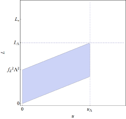
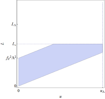
(a)(b)

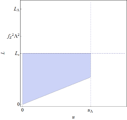
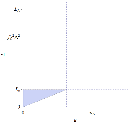
(c)(d)

Figure 1: Various possible regions of integration for $\alpha>0$. In (a) the $L_{*}>L_{\Lambda},$ where $L_{\Lambda}=\alpha u_{\Lambda}+f_{Z}^{2}\Lambda^{2}$ and $u_{\Lambda}=\textrm{min}\left(\Lambda^{2}f_{X}^{2},\Lambda^{2}f_{Y}^{2}/\widehat{K}_{\xi}^{2}\right)$ so the region is cut off at $u_{\Lambda}$. In (b) $f_{Z}^{2}\Lambda^{2}<L_{*}<L_{\Lambda}$. In (c), $L_{*}<f_{Z}^{2}\Lambda^{2}$, and $u_{\Lambda}<L_{*}/\alpha$. Finally, (d) shows a region where $L_{*}<f_{Z}^{2}\Lambda^{2}$ and $u_{\Lambda}>L_{*}/\alpha$.

3.3.1 The case $\alpha>0$

The delta function in (63) arising from the tadpole condition is $\delta\left(\widetilde{L}-\alpha u-v\right)$. This constrains the value of $v$ to be $\widetilde{L}-\alpha u$, as well as constraining the region of integration on the $\widetilde{L}/u$-plane. Let’s first determine the lower bounds on $\widetilde{L}$ and $u$:

• The variables $u,v$ are positive or possibly zero and since $\alpha>0$, then $\widetilde{L}\geq 0$, fixing the lower bound of 0 for the $\widetilde{L}$ integral.

• Let $v_{\textrm{up}}=f_{Z}^{2}\Lambda^{2}$ be the upper bound on $v$. If $v_{\textrm{up}}<\widetilde{L}$, then the delta function forces the lower bound on $u$ to be $\left(\widetilde{L}-f_{Z}^{2}\Lambda^{2}\right)/\alpha$. However, if $v_{\textrm{up}}>\widetilde{L}$ then the lower bound on $u$ is 0. So in general we let the lower bound on $u$ be $u_{\textrm{down}}^{+}=\max\left(0,\frac{\widetilde{L}-f_{Z}^{2}\Lambda^{2}}{\alpha}\right)$.

Now for the upper bounds:

• If $L_{*}<\alpha u_{\Lambda}+f_{Z}^{2}\Lambda^{2}$, then it remains the upper bound for the $\widetilde{L}$ integral. If on the contrary, the inequality runs the other way, $L_{*}>\alpha u_{\Lambda}+f_{Z}^{2}\Lambda^{2}$, then the constraint $\widetilde{L}-\alpha u-v$ cannot be satisfied everywhere along the range $0<\widetilde{L}<L_{*}$, truncating this range to $0<\widetilde{L}<\alpha u_{\Lambda}+f_{Z}^{2}\Lambda^{2}$ instead. So the upper bound on the $\widetilde{L}$ integral is

  $$L_{\textrm{up}}^{+}=\textrm{min}\left(L_{*},L_{\Lambda}\right)$$

  where $L_{\Lambda}=\alpha u_{\Lambda}+f_{Z}^{2}\Lambda^{2}$.

• If, at a fixed $\widetilde{L}$, we had $\alpha u_{\Lambda}>\widetilde{L}$, then since the lower bound on $v$ is 0, this places an upper bound on $u$ of $\widetilde{L}/\alpha$. If the inequality is reversed, then the upper bound on $u$ is $u_{\Lambda}$. So, in general the upper bound on $u$ is $u_{\textrm{up}}^{+}=\min\left(u_{\Lambda},\widetilde{L}/\alpha\right)$.

Various possible regions of integration in the $\widetilde{L}/u$-plane are illustrated in figure 1.

Using the bounds described above and integrating over $v$ yields

$$\mu_{I}^{+} \propto\int_{0}^{L_{\textrm{up}}^{+}}d\widetilde{L}\int_{u_{\textrm{down}}^{+}\left(\widetilde{L}\right)}^{u_{\textrm{up}}^{+}\left(\widetilde{L}\right)}du|\det g|\left(\left(\widetilde{L}-\alpha u\right)^{2}+\beta u^{2}+\gamma u\left(\widetilde{L}-\alpha u\right)\right)$$

where and $\beta=\mu^{2}-|\sigma|^{2}$ and $\gamma=-2\mu-|\mathcal{F}|^{2}$. Then, expanding everything out and integrating over $u$, we obtain

$$\mu_{I}^{+} \propto\int_{0}^{L_{\textrm{up}}^{+}}d\widetilde{L}|\det g|\Bigg{(}\widetilde{L}^{2}\left(u_{\textrm{up}}^{+}-u_{\textrm{down}}^{+}\right)+\frac{\gamma-2\alpha}{2}\widetilde{L}\left(\left(u_{\textrm{up}}^{+}\right)^{2}-\left(u_{\textrm{down}}^{+}\right)^{2}\right)$$

$$+\frac{\alpha^{2}+\beta-\alpha\gamma}{3}\left(\left(u_{\textrm{up}}^{+}\right)^{3}-\left(u_{\textrm{down}}^{+}\right)^{3}\right)\Bigg{)}$$

where the $\widetilde{L}$ dependence of $u_{\textrm{up}}$ and $u_{\textrm{down}}$ has been suppressed in the last line.

In order to integrate over $\widetilde{L}$, we must separate the integral above into two parts since $u_{\textrm{up}}^{+}$ and $u_{\textrm{down}}^{+}$ are different functions of $\widetilde{L}$. Let $\mathscr{I}_{\textrm{up}}^{+}$ be the portion of the integral involving terms containing powers of $u_{\textrm{up}}^{+}$ and $\mathscr{I}_{\textrm{down}}^{+}$ be the portion of the integral containing $u_{\textrm{down}}^{+}$. Note that we remove the $\left|\det g\right|$ factor from these integrals. Focusing first on $\mathscr{I}_{\textrm{up}}^{+}$ we see that for $0<\widetilde{L}/\alpha<u_{\textrm{up}}^{+}\left(L_{*}\right)$, we can replace instances of $u_{\textrm{up}}^{+}\left(\widetilde{L}\right)$ in the integral with $\widetilde{L}/\alpha$, while if $u_{\textrm{up}}^{+}\left(L_{*}\right)<\widetilde{L}/\alpha$, then $u_{\textrm{up}}^{+}=u_{\Lambda}$, which is independent of $\widetilde{L}$. So $\mathscr{I}_{\textrm{up}}^{+}$ splits into integrals over the two regions:

$$\mathscr{I}_{\textrm{up}}^{+} = \int_{0}^{\alpha u_{\textrm{up}}^{+}\left(L_{*}\right)}d\widetilde{L}\left(\frac{1}{\alpha}+\frac{\gamma-2\alpha}{2\alpha^{2}}+\frac{\alpha^{2}+\beta-\alpha\gamma}{3\alpha^{3}}\right)\widetilde{L}^{3}$$ (64)

$$+ \int_{\alpha u_{\textrm{up}}^{+}\left(L_{*}\right)}^{L_{\textrm{up}}^{+}}d\tilde{L}\left(\widetilde{L}^{2}u_{\Lambda}+\frac{\gamma-2\alpha}{2}\widetilde{L}u_{\Lambda}^{2}+\frac{\alpha^{2}+\beta-\alpha\gamma}{3}u_{\Lambda}^{3}\right)$$

Integrating yields

$$\mathscr{I}_{\textrm{up}}^{+} =\left(\frac{1}{\alpha}+\frac{\gamma-2\alpha}{2\alpha^{2}}+\frac{\alpha^{2}+\beta-\alpha\gamma}{3\alpha^{3}}\right)\frac{\alpha^{4}\left(u_{\textrm{up}}^{+}\left(L_{*}\right)\right)^{4}}{4}$$

$$+\frac{\left(\left(L_{\textrm{up}}^{+}\right)^{3}-\alpha^{3}\left(u_{\textrm{up}}^{+}\left(L_{*}\right)\right)^{3}\right)u_{\Lambda}}{3}+\frac{\gamma-2\alpha}{4}\left(\left(L_{\textrm{up}}^{+}\right)^{2}-\alpha^{2}\left(u_{\textrm{up}}^{+}\left(L_{*}\right)\right)^{3}\right)u_{\Lambda}^{2}$$ (65)

$$+\frac{\alpha^{2}+\beta-\alpha\gamma}{3}\left(L_{\textrm{up}}^{+}-\alpha u_{\textrm{up}}^{+}\left(L_{*}\right)\right)u_{\Lambda}^{3}$$ (66)

For the integral $\mathscr{I}_{\textrm{down}}^{+}$, we consider the regions $0<\widetilde{L}<f_{Z}^{2}\Lambda$ and $f_{Z}^{2}\Lambda<\widetilde{L}$. In the first case, $u_{\textrm{down}}^{+}=0$ in which case this entire portion of the integral vanishes, while in the second, $u_{\textrm{down}}^{+}=\left(\widetilde{L}-f_{Z}^{2}\Lambda\right)/\alpha$. If $L_{*}<f_{Z}^{2}\Lambda^{2}$ then the entirety of $\mathscr{I}_{\textrm{down}}^{+}=0$, so we have

$$\mathscr{I}_{\textrm{down}}^{+} =-\theta\left(L_{*}-f_{Z}^{2}\Lambda^{2}\right)\int_{f_{Z}^{2}\Lambda^{2}}^{L_{\textrm{up}}^{+}}d\widetilde{L}\Bigg{(}\frac{1}{\alpha}\left(\widetilde{L}^{3}-f_{Z}^{2}\Lambda^{2}\widetilde{L}^{2}\right)+\frac{\gamma-2\alpha}{2\alpha^{2}}\left(\widetilde{L}^{3}-2f_{Z}^{2}\Lambda^{2}\widetilde{L}^{2}+f_{Z}^{4}\Lambda^{4}\widetilde{L}\right)$$

$$+\frac{\alpha^{2}+\beta-\alpha\gamma}{3\alpha^{3}}\left(\widetilde{L}^{3}-3f_{Z}^{2}\Lambda^{2}\widetilde{L}^{2}+3f_{Z}^{4}\Lambda^{4}\widetilde{L}-f_{Z}^{6}\Lambda^{6}\right)\Bigg{)}$$

$$=-\theta\left(L_{*}-f_{Z}^{2}\Lambda^{2}\right)\int_{f_{Z}^{2}\Lambda^{2}}^{L_{\textrm{up}}^{+}}d\widetilde{L}\Bigg{(}\left(\frac{1}{\alpha}+\frac{\gamma-2\alpha}{2\alpha^{2}}+\frac{\alpha^{2}+\beta-\alpha\gamma}{3\alpha^{3}}\right)\widetilde{L}^{3}$$

$$-f_{Z}^{2}\Lambda^{2}\left(\frac{1}{\alpha}+\frac{\gamma-2\alpha}{\alpha^{2}}+\frac{\alpha^{2}+\beta-\alpha\gamma}{\alpha^{3}}\right)\widetilde{L}^{2}$$

$$+f_{Z}^{4}\Lambda^{4}\left(\frac{\gamma-2\alpha}{2\alpha^{2}}+\frac{\alpha^{2}+\beta-\alpha\gamma}{\alpha^{3}}\right)\widetilde{L}-f_{Z}^{6}\Lambda^{6}\frac{\alpha^{2}+\beta-\alpha\gamma}{3\alpha^{3}}\Bigg{)}$$

Integrating yields

$$\mathscr{I}_{\textrm{down}}^{+} =-\theta\left(L_{*}-f_{Z}^{2}\Lambda^{2}\right)\Bigg{(}f_{Z}^{8}\Lambda^{8}\left(\frac{1}{12\alpha}-\frac{\gamma-2\alpha}{24\alpha^{2}}+\frac{\alpha^{2}+\beta-\alpha\gamma}{12\alpha^{3}}\right)$$

$$-f_{Z}^{6}\Lambda^{6}\frac{\alpha^{2}+\beta-\alpha\gamma}{3\alpha^{3}}L_{\textrm{up}}^{+}+f_{Z}^{4}\Lambda^{4}\left(\frac{\gamma-2\alpha}{4\alpha^{2}}+\frac{\alpha^{2}+\beta-\alpha\gamma}{2\alpha^{3}}\right)\left(L_{\textrm{up}}^{+}\right)^{2}$$

$$-\frac{1}{3}f_{Z}^{2}\Lambda^{2}\left(\frac{1}{\alpha}+\frac{\gamma-2\alpha}{\alpha^{2}}+\frac{\alpha^{2}+\beta-\alpha\gamma}{\alpha^{3}}\right)\left(L_{\textrm{up}}^{+}\right)^{3}+\left(\frac{1}{4\alpha}+\frac{\gamma-2\alpha}{8\alpha^{2}}+\frac{\alpha^{2}+\beta-\alpha\gamma}{12\alpha^{3}}\right)\left(L_{\textrm{up}}^{+}\right)^{4}\Bigg{)}$$

Notice that when one ignores warping and the finite fluxes, $\alpha=1,\widehat{K}_{\xi}=0$, and $\Lambda\rightarrow\infty$, implying $\beta=1$, $\gamma=-2-\left|\mathcal{F}\right|^{2}$, $u_{\textrm{up}}^{+}\left(L_{*}\right)=L_{*}$, and $L_{\textrm{up}}^{+}=L_{*}$. In this case, we must go back to the expression (64) and note that the second integral in that expression vanishes since the lower and upper bound of integration are both $L_{*}$. Furthermore the integral $\mathscr{I}_{\textrm{down}}^{+}$ vanishes due to the $\theta$-function prefactor. The index density in the unwarped case is thus

$$\mu_{I}^{\text{Unwarped}}(\xi,\tau)=\left|\det g\right|\mathscr{I}_{\textrm{up}}^{+}=\left|\det g\right|\frac{L_{*}^{4}}{4}\left(\frac{6+3\gamma-6+2+2\beta-2\gamma}{6}\right)=\left|\det g\right|\frac{L_{*}^{4}}{4!}(2-|\mathcal{F}|^{2})$$ (67)

This precise combination gives us the curvature tensor as argued in [3, 4]. So, our expression reduces to the correct form in the unwarped, infinite flux case. We now turn our attention to the case where $\alpha<0$.

3.3.2 The case $\alpha<0$

Once again, we first establish the lower and upper bounds on $\widetilde{L}$ and $u$:

• Suppose we are at the lower bound on $v$, namely $v=0$. In this case, the tadpole constraint $\widetilde{L}-\alpha u-v=0$ tells us that the lower bound attained by $\widetilde{L}$ is $L_{\textrm{down}}^{-}=\alpha u_{\Lambda}$. Note that this is negative.

• Consider some fixed $\widetilde{L}\leq f_{Z}^{2}\Lambda^{2}$; If $\widetilde{L}>0$, then there is always a $v=\widetilde{L}$ to cancel it, and the lower bound for $u$ in this case is 0. However, if $\widetilde{L}<0$, the fact that $v\geq 0$ implies that for the constraint to hold, we need the lower bound for $u$ to be $\widetilde{L}/\alpha$. So in general, the lower bound for $u$ is $u_{\textrm{down}}^{-}=\max\left(0,\widetilde{L}/\alpha\right)$.

• By similar reasoning to the previous case, if $L_{*}<f_{Z}^{2}\Lambda^{2}$, then it may remain the upper bound on $\widetilde{L}$. However, if $L_{*}>f_{Z}^{2}\Lambda^{2}$, then the upper bound on $\widetilde{L}$ becomes $f_{Z}^{2}\Lambda^{2}$. So in general, the upper bound on $\widetilde{L}$ is $L_{\textrm{up}}^{-}=\min(L_{*},f_{Z}^{2}\Lambda^{2})$.

• Consider again a fixed $\widetilde{L}$, and suppose $v$ is at its upper bound of $f_{Z}^{2}\Lambda^{2}$. If $\alpha u_{\Lambda}>\widetilde{L}-f_{Z}^{2}\Lambda^{2}$, then the upper bound of $u$ must be truncated to $\left(\widetilde{L}-f_{Z}^{2}\Lambda^{2}\right)/\alpha$. Otherwise, if $\alpha u_{\Lambda}<\widetilde{L}-f_{Z}^{2}\Lambda^{2}$, then the upper bound on $u$ remains $u_{\Lambda}$. In general then, $u_{\textrm{up}}^{-}=\min\left(u_{\Lambda},\left(\widetilde{L}-f_{Z}^{2}\Lambda^{2}\right)/\alpha\right)$.

Given these bounds on $u$ and $\widetilde{L}$, we may now integrate over $v$, eliminating the tadpole delta function to get

$$\mu_{I}^{-}\propto\int_{L_{\textrm{down}}^{-}}^{L_{\textrm{up}}^{-}}d\widetilde{L}\int_{u_{\textrm{down}}^{-}\left(\widetilde{L}\right)}^{u_{\textrm{up}}^{-}\left(\widetilde{L}\right)}du\,|\det g|\,\left(\widetilde{L}^{2}+(\gamma-2\alpha)\widetilde{L}u+\left(\alpha^{2}+\beta-\alpha\gamma\right)u^{2}\right)$$ (68)

Carrying out the $u$ integration yields

$$\mu_{I}^{-} \propto \int_{L_{\textrm{down}}^{-}}^{L_{\textrm{up}}^{-}}d\widetilde{L}|\det g|\,\Bigg{(}\widetilde{L}^{2}\left(u_{\textrm{up}}^{-}-u_{\textrm{down}}^{-}\right)+\widetilde{L}\left(\frac{\gamma-2\alpha}{2}\right)\left(\left(u_{\textrm{up}}^{-}\right)^{2}-\left(u_{\textrm{down}}^{-}\right)^{2}\right)$$ (69)

$$+ \frac{\alpha^{2}+\beta-\alpha\gamma}{3}\left(\left(u_{\textrm{up}}^{-}\right)^{3}-\left(u_{\textrm{down}}^{-}\right)^{3}\right)\Bigg{)}$$

where we have suppressed the $\widetilde{L}$ dependence of $u_{\textrm{up}}^{-}$, and $u_{\textrm{down}}^{-}$.

As before, split the integral into two parts, $\mathscr{I}_{\textrm{up}}^{-}$ and $\mathscr{I}_{\textrm{down}}^{-}$, involving just the $u_{\textrm{up}}^{-}$ and $u_{\textrm{down}}^{-}$ parts, respectively. To compute $\mathscr{I}_{\textrm{up}}^{-}$ we consider two cases:

• Suppose $L_{*}<L_{\Lambda}$, where we recall $L_{\Lambda}=\alpha u_{\Lambda}+f_{Z}^{2}\Lambda^{2}$. Note that since $\alpha<0$, we have that $L_{\Lambda}<f_{Z}^{2}\Lambda^{2}$, and thus, $L_{\textrm{up}}^{-}=L_{*}$ in this case. We also see that $u_{\textrm{up}}^{-}=u_{\Lambda}$, and so in this case, the integral $\mathscr{I}_{\textrm{up}}^{-}$ is simply

  $$\mathscr{I}_{\textrm{up}}^{-}=\int_{L_{\textrm{down}}^{-}}^{L_{*}}d\widetilde{L}\Bigg{(}\widetilde{L}^{2}u_{\Lambda}+\widetilde{L}\left(\frac{\gamma-2\alpha}{2}\right)u_{\Lambda}^{2}+\frac{\alpha^{2}+\beta-\alpha\gamma}{3}u_{\Lambda}^{3}\Bigg{)}$$

• Suppose that $L_{*}>L_{\Lambda}$. In this case, for $\widetilde{L}<L_{\Lambda}$, $u_{\textrm{up}}^{-}=u_{\Lambda}$ as before, but when $\widetilde{L}>L_{\Lambda}$ we have $u_{\textrm{up}}^{-}=\left(\widetilde{L}-f_{Z}^{2}\Lambda^{2}\right)/\alpha$. So the integral splits into two parts

  $$\mathscr{I}_{\textrm{up}}^{-} = \int_{L_{\textrm{down}}^{-}}^{L_{\Lambda}}d\widetilde{L}\Bigg{(}\widetilde{L}^{2}u_{\Lambda}+\widetilde{L}\left(\frac{\gamma-2\alpha}{2}\right)u_{\Lambda}^{2}+\frac{\alpha^{2}+\beta-\alpha\gamma}{3}u_{\Lambda}^{3}\Bigg{)}$$ (70)

  $$+ \int_{L_{\Lambda}}^{L_{\textrm{up}}^{-}}d\widetilde{L}\Bigg{(}\widetilde{L}^{2}\left(\frac{\widetilde{L}-f_{Z}^{2}\Lambda^{2}}{\alpha}\right)+\widetilde{L}\left(\frac{\gamma-2\alpha}{2}\right)\left(\frac{\widetilde{L}-f_{Z}^{2}\Lambda^{2}}{\alpha}\right)^{2}$$

  $$+ \frac{\alpha^{2}+\beta-\alpha\gamma}{3}\left(\frac{\widetilde{L}-f_{Z}^{2}\Lambda^{2}}{\alpha}\right)^{3}\Bigg{)}$$

These two expressions can be joined if we introduce $L_{\textrm{mid}}=\min\left(L_{*},L_{\Lambda}\right)$:

$$\mathscr{I}_{\textrm{up}}^{-} = \int_{L_{\textrm{down}}^{-}}^{L_{\textrm{mid}}}d\widetilde{L}\Bigg{(}\widetilde{L}^{2}u_{\Lambda}+\widetilde{L}\left(\frac{\gamma-2\alpha}{2}\right)u_{\Lambda}^{2}+\frac{\alpha^{2}+\beta-\alpha\gamma}{3}u_{\Lambda}^{3}\Bigg{)}$$ (71)

$$+ \int_{L_{\textrm{mid}}}^{L_{\textrm{up}}^{-}}d\widetilde{L}\Bigg{(}\widetilde{L}^{2}\left(\frac{\widetilde{L}-f_{Z}^{2}\Lambda^{2}}{\alpha}\right)+\left(\frac{\gamma-2\alpha}{2}\right)\widetilde{L}\left(\frac{\widetilde{L}-f_{Z}^{2}\Lambda^{2}}{\alpha}\right)^{2}$$

$$+ \frac{\alpha^{2}+\beta-\alpha\gamma}{3}\left(\frac{\widetilde{L}-f_{Z}^{2}\Lambda^{2}}{\alpha}\right)^{3}\Bigg{)}$$

The integral in the second line above vanishes if $L_{\textrm{mid}}=L_{*}$, since in that case $L_{\textrm{up}}^{-}$ also is $L_{*}$. Carrying out the integral yields (after plugging in $L_{\textrm{down}}^{-}=\alpha u_{\Lambda}$)

$$\mathscr{I}_{\textrm{up}}^{-} = \frac{u_{\Lambda}}{3}\bigg{(}L_{\textrm{mid}}^{3}-\alpha^{3}u_{\Lambda}^{3}\bigg{)}+\frac{\gamma-2\alpha}{4}u_{\Lambda}^{2}\bigg{(}L_{\textrm{mid}}^{2}-\alpha^{2}u_{\Lambda}^{2}\bigg{)}+\frac{\alpha^{2}+\beta-\alpha\gamma}{3}u_{\Lambda}^{3}\left(L_{\textrm{mid}}-\alpha u_{\Lambda}\right)$$

$$+ \frac{1}{4}\left(\frac{1}{\alpha}+\frac{\gamma-2\alpha}{2\alpha^{2}}+\frac{\alpha^{2}+\beta-\alpha\gamma}{3\alpha^{3}}\right)\left(\left(L_{\textrm{up}}^{-}\right)^{4}-L_{\textrm{mid}}^{4}\right)$$

$$- \frac{f_{Z}^{2}\Lambda^{2}}{3}\left(\frac{1}{\alpha}+\frac{\gamma-2\alpha}{\alpha^{2}}+\frac{\alpha^{2}+\beta-\alpha\gamma}{\alpha^{3}}\right)\left(\left(L_{\textrm{up}}^{-}\right)^{3}-L_{\textrm{mid}}^{3}\right)$$

$$+ \frac{f_{Z}^{4}\Lambda^{4}}{2}\left(\frac{\gamma-2\alpha}{2\alpha^{2}}+\frac{\alpha^{2}+\beta-\alpha\gamma}{\alpha^{3}}\right)\left(\left(L_{\textrm{up}}^{-}\right)^{2}-L_{\textrm{mid}}^{2}\right)$$

$$- f_{Z}^{6}\Lambda^{6}\left(\frac{\alpha^{2}+\beta-\alpha\gamma}{3\alpha^{3}}\right)\left(L_{\textrm{up}}^{-}-L_{\textrm{mid}}\right)$$

The integral $\mathscr{I}_{\textrm{down}}^{-}$ vanishes when $\widetilde{L}>0$ since in that case $u_{\textrm{down}}^{-}=0$. Thus, the only region that contributes is where $L_{\textrm{down}}^{-}\leq\widetilde{L}\leq 0$, in which $u_{\textrm{down}}^{-}=\widetilde{L}/\alpha$. We have,

$$\mathscr{I}_{\textrm{down}}^{-}=-\int_{L_{\textrm{down}}^{-}}^{0}d\widetilde{L}\left(\frac{1}{\alpha}\tilde{L}^{3}+\frac{\gamma-2\alpha}{2\alpha^{2}}\tilde{L}^{3}+\frac{\alpha^{2}+\beta-\alpha\gamma}{3\alpha^{3}}\tilde{L}^{3}\right)$$

which gives

$$\mathscr{I}_{\textrm{down}}^{-}=\frac{1}{4}\left(\frac{1}{\alpha}+\frac{\gamma-2\alpha}{2\alpha^{2}}+\frac{\alpha^{2}+\beta-\alpha\gamma}{3\alpha^{3}}\right)\alpha^{4}u_{\Lambda}^{4}$$

where we have again used $L_{\textrm{down}}^{-}=\alpha u_{\Lambda}$.

The full index density is thus

$$\mu_{I}(\xi,\tau)/\det g=\left(\mathscr{I}_{\textrm{up}}^{+}+\mathscr{I}_{\textrm{down}}^{+}\right)\theta(\alpha)+\left(\mathscr{I}_{\textrm{up}}^{-}+\mathscr{I}_{\textrm{down}}^{-}\right)\theta(-\alpha)$$ (72)

In the unwarped, infinite flux case where a consise geometric result is obtained, one can integrate out the axio-dilaton to obtain an effective density only in terms of the complex moduli. However, in our case this type of integration proves intractable. As a result we will when comparing with simulations have to fix a value of the axio-dilaton and compare the un-integrated form of our density.

4 Numerical Vacuum Statistics

To perform a numerical study of the distribution of vacua in moduli space near the conifold point, we will randomly choose appropriate fluxes $F=(F_{0},F_{1},F_{2},F_{3})$ and $H=(H_{0},H_{1},H_{2},H_{3})$ and then solve the conditions $D_{\tau}W=0$ and $D_{\xi}W=0$ for the moduli space coordinate $\xi$. Here $W=N_{i}\Pi_{i}$ is the superpotential, and $N$ is an 8-vector whose first four components are those of $F$ and last four are those of $H$. We work in a basis such that the vector of 4-fold periods $\Pi=\left(\Sigma,\tau\Sigma\right)$, where $\Sigma$ is the vector of periods on the 3-fold. Near the conifold point, the vector of 3-fold periods takes the form:

$$\Sigma=\sum_{n=0}^{\infty}a_{n}\xi^{n}+b\xi\log(-i\xi),$$ (73)

where the $a_{n}$ and $b$ are constant vectors associated with the expansion of the periods. Note that in the case of a single complex modulus, the vector $b=(0,0,0,b^{0})$, since only $\Sigma_{0}$ has non-trivial logarithmic behavior near the conifold. Also, the local coordinate around the conifold point is proportional to $\Sigma_{3}$, which implies that the vector $a_{0}=(0,a_{0}^{2},a_{0}^{1},a_{0}^{0})$.

4.1 Unwarped Analysis

The unwarped Kähler potential is

$$e^{-K}=-i\overline{\Sigma}\cdot Q\cdot\Sigma=-i\left((\overline{a}_{n}\cdot Q\cdot a_{m})\bar{\xi}^{n}\xi^{m}+(\overline{b}\cdot Q\cdot a_{m})\xi^{m}\bar{\xi}\log(i\overline{\xi})+(\overline{a}_{n}\cdot Q\cdot b)\bar{\xi}^{n}\xi\log(-i\xi)\right),$$ (74)

where the term proportional to $\overline{b}\cdot Q\cdot b$ has been dropped since given $b$ and $\eta$ it vanishes.

For SUSY vacua in the unwarped case

$$D_{\xi}W=N\cdot(\partial_{\xi}\Pi+\Pi K_{\xi})=0.$$ (75)

Keeping logarithmic and constant terms gives

$$(F-\tau H)\cdot\left(a_{1}+b\left(\log(-i\xi)+1\right)\right)-(F-\tau H)\cdot a_{0}\frac{\overline{a}_{0}\cdot Q\cdot a_{1}}{\overline{a}_{0}\cdot Q\cdot a_{0}}=0.$$ (76)

where the fact that $\overline{a}_{0}\cdot Q\cdot b=0$ has been used to simplify the expression. This is an equation of the form

$$\mathcal{A}+\mathcal{B}\log(-i\xi)=0,$$ (77)

with

$$\mathcal{A} = \frac{1}{c}(F-\tau H)\cdot b(\overline{a}_{0}\cdot Q\cdot a_{0})+(F-\tau H)\cdot a_{1}(\overline{a}_{0}\cdot Q\cdot a_{0})-(F-\tau H)\cdot a_{0}(\overline{a}_{1}\cdot Q\cdot a_{0})$$ (78)

$$\mathcal{B} = (F-\tau H)\cdot b(\overline{a}_{0}\cdot Q\cdot a_{0}).$$ (79)

The leading-order constraints arising from requiring $D_{\tau}W=0$ are

$$\tau=\frac{F\cdot\overline{\Sigma}}{H\cdot\overline{\Sigma}}=\frac{F\cdot\overline{a}_{0}}{H\cdot\overline{a}_{0}}.$$ (80)

This implies that

$$F-\tau H=\frac{(H\cdot\overline{a}_{0})F-(F\cdot\overline{a}_{0})H}{H\cdot\overline{a}_{0}}$$ (81)

Before considering the effects of warp corrections, it’s worth determining how close to the conifold vacua may be found in the unwarped scenario. The $D_{\xi}W=0$ constraint implies that $|c\xi|$ is exponentially suppressed by the ratio of $|\mathcal{A}/\mathcal{B}|$, so if $|\mathcal{A}|$ is even just a couple of orders of magnitude greater than $|\mathcal{B}|$, we should expect to see vacua on the order of $10^{-100}$ units away from the conifold point—indeed, this has been observed in previous studies. In order for $|\mathcal{A}|$ to differ appreciably from $|\mathcal{B}|$ the quantity $|(F-\tau H)\cdot b|$ should be relatively small compared to $|(F-\tau H)\cdot a_{0}|$ or $|(F-\tau H)\cdot a_{1}|$. Using the form of the vector $b$ above, this indicates that the fluxes through the collapsing cycle, $F_{3}$ and $H_{3}$ should be small relative to some of the other fluxes.

4.2 Warped Analysis

Introducing warping leads to the corrections (48) and (49) to the Kähler potential and its derivative. The modification to the near-conifold SUSY vacuum condition is then

$$D_{\xi}W\longrightarrow D_{\xi}W+3C_{w}\frac{\bar{\xi}^{1/3}}{\xi^{2/3}}N\cdot\Pi.$$ (82)

Now, assuming that $C_{w}$ is small (i.e. the volume of the 3-fold is large) these new terms will matter only close to $\xi=0$. The SUSY condition thus leads to

$$\mathcal{A}+\mathcal{B}\log(-i\xi)+\mathcal{C}\frac{\bar{\xi}^{1/3}}{\xi^{2/3}}=0,$$ (83)

with $\mathcal{A}$ and $\mathcal{B}$ as before and

$$\mathcal{C}=3\,C_{w}(F-\tau H)\cdot a_{0}.$$ (84)

From this, we can see the rough influence of warping on the distribution of vacua. In the unwarped case, we expect to find vacua $10^{-100}$ or so away from the conifold with fluxes yielding $|\mathcal{A}|\sim 100|\mathcal{B}|$ (which with fluxes constrained to lie in $(0,100$ is about the maximum order of magnitude difference that we expect.) If however, $C_{w}\sim 10^{-20}$, then for $|\xi|\sim 10^{-100}$, the warp term contribution is on the order of $10^{10}$, swamping the logarithmic contribution and requiring fluxes $|\mathcal{A}|\sim 10^{10}$ which lies beyond the range we consider.

In the region of strong warping where the logarithmic term is dominated by the warping term, the distance of a vacuum from the conifold point is thus set by $|\mathcal{C}/\mathcal{A}|^{3}$. Given that $\mathcal{A}$ is at maximum of roughly 100 or so, the constant $C_{w}$, and thus, the overall volume of the Calabi-Yau, determines how near the conifold vacua lie. This can dramatically truncate the range—since the assumption of large but finite volume is well satisfied by volumes of order $10^{20}$, but in those cases, vacua will not show up much closer than $10^{-60}$. We can get vacua at around $10^{-120}$ by taking a volume of order $10^{40}$, but in the absence of warping, vacua as far in as $10^{-200}$ are expected. Thus, warping pushes vacua away from the conifold point.

4.3 Monte-Carlo vacua

For the numerical analysis, we use the Calabi-Yau manifold labeled model 3 in the appendix of [1]. This family of Calabi-Yau can be expressed as a locus of octic polynomials in $\mathbb{WP}^{4,1,1,1,1}$. The corresponding orientifold arises from a certain limit of F-theory compactified on a Calabi-Yau fourfold hypersurface in $\mathbb{WP}^{12,8,1,1,1,1},$ following the methods of [10], and briefly described in [11]. For our purposes, we use the fact that the fourfold has Euler characteristic $\chi=23328$, which implies that $L_{\textrm{max}}=\chi/24=972$ for the tadpole condition for flux compactification on the corresponding orientifolded 3-fold.

Since the warped form of the near conifold equation is not as simple to solve as in the unwarped case, a slightly more involved approach is necessary. We begin by defining two real variables $\rho$ and $\theta$ such that

$$-i\xi=\rho^{3}e^{i\theta}$$ (85)

We take $\rho\geq 0$ and $0\leq\theta\leq 2\pi$. In terms of these variables, eqn (83) and its complex conjugate expression take the form

$$\mathcal{A}+3\mathcal{B}\ln(\rho)+i\mathcal{B}\theta+\frac{\mathcal{C}}{\rho}e^{-i\theta} = 0$$ (86)

$$\overline{\mathcal{A}}+3\overline{\mathcal{B}}\ln(\rho)-i\overline{\mathcal{B}}\theta+\frac{\overline{\mathcal{C}}}{\rho}e^{i\theta} = 0$$ (87)

Multiplying the first equation by $\overline{\mathcal{B}}$ and the second one by $\mathcal{B}$, and then adding and subtracting the two, we find two purely real or imaginary equations. Letting $\mathcal{A}=ae^{i\alpha}$, $\mathcal{B}=be^{i\beta}$, and $\mathcal{C}=ce^{i\gamma}$, we have

$$a\sin(\alpha-\beta)+b\theta+\frac{c}{\rho}\sin(\gamma-\beta-\theta) = 0$$ (88)

$$a\cos(\alpha-\beta)+3b\log(\rho)+\frac{c}{\rho}\cos(\gamma-\beta-\theta) = 0$$ (89)

We now solve for $\rho$ in terms of $\theta$ and then numerically solve the final equation for $\theta$. It seems natural to solve equation (88) for $\rho$ since it is a linear equation. However, this approach fails in the limit $C_{w}\rightarrow 0$ since then $c\rightarrow 0$ too. Instead we solve for $\rho$ in equation (89). One can rearrange the equation as

$$\rho e^{\Gamma}\log(\rho e^{\Gamma})=-\frac{ce^{\Gamma}}{3b}\cos(\gamma-\beta-\theta)$$ (90)

Here we have defined the constant $\Gamma=\frac{a\cos(\alpha-\beta)}{3b}$. This is of the form $x\log(x)=y$ which has the solution $x=y/W(y)$ where $W(y)$ is the Lambert $W$-function. We therefore find

$$\rho(\theta)=\frac{-c\cos(\gamma-\beta-\theta)}{3bW(-\frac{ce^{\Gamma}}{3b}\cos(\gamma-\beta-\theta))}$$ (91)

Consider equation (88), which now only depends on $\theta$. Under the assumption that there is only one near conifold vacuum for each set of fluxes, the left hand side must either start out positive, and go negative or vice versa. To find the zero-crossing, we divide the region $[0,2\pi]$ into two equally pieces and then determine in which region (if any) equation (88) changes sign. If such a region is found, we apply the same method to that region, splitting it into two smaller intervals, continuing in this way until we reach a predetermined level of accuracy. There are two relevant comments. First, in equation (91) it is not clear that the value of $\rho$ is real, or even positive. We must therefore exclude the regions where $\rho$ is either negative or complex. Fortunately, if $\rho$ is real, it is never negative since $W(x)$ must have the same sign as $x$. A necessary and sufficient condition for $\rho$ to be real is that the argument of the Lambert $W$ function is greater than or equal to $-1/e$. This means that the relevant region to begin with may not be the entire interval $[0,2\pi]$. Second, it turns out that the Lambert $W$ function has two real branches for arguments between $-1/e$ and $0$. Thus, both of these branches must be considered.

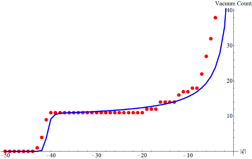
Figure 2: A comparison between numerical and analytical distributions. Red circles mark the numerical data while the blue curve is the integrated analytical distribution. Distance from the conifold $\left|\xi\right|$ is plotted on a log scale on the horizontal axis, while the vacuum count is plotted on the vertical axis.

To better compare the numerical and analytical and numerical distributions, we fix $\tau$ and then select a random sets of fluxes $F$ and $H$ consistent with our choice of $\tau$ and satisfying the tadpole condition, $F\cdot Q\cdot H\leq L_{max}$. For the particular model we consider, $L_{max}=972$, and we display a run using $\tau=2i$, and $C_{w}=10^{-15}$ in figure 2. The figure shows a numerical run compared to the analytical distribution. We plot the vacuum count and integrated analytical distribution as measured around the conifold point using a log scale for the distance from the conifold. As is evident from the figure, the count receives two major contributions: the one farther away from the conifold point is the usual contribution that is present without warping. However, we also see a major contribution much closer to the conifold at a distance roughly on the order of $C_{w}^{3}$. This contribution is due to the strong warping effects and is matched by the cumulative analytical results.

5 Discussion

We’ve analyzed the distribution of flux vacua in the vicinity of the conifold point, including the effects of warping, and confirmed our results by a direct numerical Monte Carlo search. In comparison with the well known results, that don’t include warping, we find a significant dilution of vacua in close proximity to the conifold, with the proximity scale set by the volume of the Calabi-Yau compactification.

One complication in the analytical approach, relative to the unwarped case, is the need to bound the fluxes – a physically sensible requirement but one that can be avoided in the unwrapped analysis, yielding the geometrical result of [3, 4]. It would be interesting to see whether the warped distribution of vacua can once again be related to intrinsic properties of the moduli space through a more complete geometrical treatment, likely requiringing careful consideration of the generalized complex geometry of conformal Calabi-Yau spaces [6, 7].

Acknowledgements

We thank Michael Douglas, Saswat Sarangi, Gary Shiu, and I-Sheng Yang for helpful discussions. Pontus Ahlqvist is partly supported by a graduate fellowship from the Sweden America Foundation. This work is supported in part by DOE grant DE-FG02-92ER40699, FQXi grant RFP1-06-19, and STARS grant CHAPU G2009-30 7557.

Appendix A Appendix

A.1 Covariant Derivatives

We start with the standard definition of the Kähler potential

$$e^{-K}=\int\widehat{\Omega}_{4}\wedge\overline{\widehat{\Omega}}_{4}$$

A rescaling of the holomorphic 4-form $\widehat{\Omega}_{4}\rightarrow e^{f(z)}\widehat{\Omega}_{4}$ implies that $K\rightarrow K-f(z)-\overline{f(z)}$. The covariant derivative is defined so that it is covariant under such rescalings:

$$D_{a}\widehat{\Omega}_{4}\rightarrow e^{f(z)}D_{a}\widehat{\Omega}_{4}=\left(D_{a}-\partial_{a}f\right)\left(e^{f(z)}\widehat{\Omega}_{4}\right)$$

implying that $D_{a}\widehat{\Omega}_{4}=\left(\partial_{a}+K_{a}\right)\widehat{\Omega}_{4}$. Note also that the holomorphic covariant derivative annihilates antiholomorphic objects, i.e. $D_{a}\overline{\widehat{\Omega}}_{4}=\partial_{a}\overline{\widehat{\Omega}}_{4}=0$. We see then that

$$D_{a}e^{-K}=\left(\partial_{a}+K_{a}\right)e^{-K}=0$$

Notice that covariance dictates that

$$D_{a}e^{K}=\left(\partial_{a}-K_{a}\right)e^{K}=0$$

In addition to this Kähler scaling structure, the complex structure moduli space is a manifold with a natural Kähler metric $K_{a\bar{b}}=\partial_{a}\partial_{\bar{b}}K$. We can thus define a metric compatible connection via

$$\Gamma_{bc}^{a}=K^{a\bar{d}}K_{\bar{d}bc}$$

where $K_{\bar{d}bc}=\partial_{c}K_{\bar{d}b}$. Note that the connection components with mixed holomorphic and antiholomorphic indices vanish. By suitably extending the covariant derivative $D_{a}$, we can ensure that it transforms covariantly under both Kähler rescalings and coordinate transformations on the complex moduli space. In particular, since the connection is metric compatible, $D_{a}K_{b\bar{c}}=0$.

The superpotential

$$\widehat{W}=\int G_{4}\wedge\widehat{\Omega}_{4}$$

scales as $\widehat{\Omega}_{4}$, and thus

$$D_{a}\widehat{W}=\partial_{a}\widehat{W}+K_{a}\widehat{W}$$

A supersymmetric vacuum satisfies the conditions $D_{a}\widehat{W}=0$. The components of the fermion mass matrix are

$$\partial_{a}D_{b}\widehat{W}=\partial_{a}\partial_{b}\widehat{W}+K_{ab}\widehat{W}+K_{b}\widehat{W}_{a}$$

Notice that at a generic point in the moduli space the quantity

$$D_{a}D_{b}\widehat{W}=\partial_{a}D_{b}\widehat{W}+K_{a}D_{b}\widehat{W}-\Gamma_{ab}^{c}D_{c}\widehat{W}=\partial_{a}D_{b}\widehat{W}+K_{a}D_{b}\widehat{W}-K_{ab\bar{d}}K^{\bar{d}c}D_{c}\widehat{W}$$

does not equate to the fermion mass matrix. However, the extra terms drop out at supersymmetric vacua.

Now let $\widehat{\Omega}_{4}\rightarrow\Omega_{4}=e^{K/2}\widehat{\Omega}_{4}$ and similarly for the (0,4)-form. Notice that the scaling properties of $\Omega_{4}$ imply that

$$D_{a}\Omega_{4}=\left(\partial_{a}+\frac{1}{2}K_{a}\right)\Omega_{4}=\left(\partial_{a}+\frac{1}{2}K_{a}\right)\left(e^{K/2}\widehat{\Omega}_{4}\right)=e^{K/2}\left(\partial_{a}+K_{a}\right)\widehat{\Omega}_{4}=e^{K/2}D_{a}\widehat{\Omega}_{4}$$

The rescaled (4,0) and (0,4) forms are convenient since they remove factors of $e^{K}$ from various expressions. In particular we have

$$\int\Omega_{4}\wedge\overline{\Omega}_{4}=1$$

We can also go to an orthonormal frame by introducing vielbeins $\delta_{A\overline{B}}=e_{A}^{a}e_{\overline{B}}^{\overline{b}}K_{a\bar{b}}$. The covariant derivative must be extended so as to keep the vielbeins covariantly constant:

$$D_{a}e_{B}^{b}=\partial_{a}e_{B}^{b}+K^{b\bar{d}}K_{\bar{d}ac}e_{B}^{c}-\omega_{aB}{}^{C}e_{C}^{b}=0$$

implying that

$$\omega_{AB}{}^{C}=e_{A}^{a}\omega_{aB}{}^{C}=e_{b}^{C}e_{A}^{a}\partial_{a}e_{B}^{b}+K^{b\bar{d}}K_{\bar{d}ac}e_{A}^{a}e_{B}^{c}e_{b}^{C}$$

Given these definitions, we can now go to rescaled expressions in the orthonormal frame:

$$D_{A}D_{B}W=\partial_{A}D_{B}W+K_{A}D_{B}W-\omega_{AB}{}^{C}D_{C}W$$

once again, the expression above agrees with the fermion mass matrix components evaluated at a vacuum.

A.2 Computations

In this section, we provide derivations for the equations (31)-(38). To do so, recall from equation (30) that the flux four form written in the basis $\mathcal{B}=\{\Omega_{4},D_{A}\Omega_{4},D_{\underline{0}}D_{I}\Omega_{4},\overline{\Omega}_{4},\overline{D_{A}\Omega}_{4},\overline{D_{\underline{0}}D_{I}\Omega}_{4}\}$ is

$$G_{4}=\overline{X}\Omega_{4}-\overline{Y}{}^{A}D_{A}\Omega_{4}+\overline{Z}{}^{I}D_{\underline{0}}D_{I}\Omega_{4}+\text{c.c.}$$ (92)

It’s useful to note that $D_{A}D_{B}\Omega_{4}$ is a (2,2)-form. In fact, given the nature of our Calabi-Yau 4-fold, essentially factorizing into a 3-fold and a torus, this (2,2)-form can be decomposed as $(2,2)=(1,0)\wedge(1,2)\oplus(0,1)\wedge(2,1)$. To see this, note that $D_{A}\Omega_{4}$ could be a mixture of a $(3,1)\oplus(4,0)$, but the (4,0) component vanishes:

$$\int_{\mathcal{M}}D_{A}\Omega_{4}\wedge\overline{\Omega}_{4}=D_{A}\left(\int_{\mathcal{M}}\Omega_{4}\wedge\overline{\Omega}_{4}\right)-\int_{\mathcal{M}}\Omega_{4}\wedge D_{A}\overline{\Omega}_{4}=0$$

where the two terms vanish given the properties of the covariant derivative defined above. Similarly $D_{A}D_{B}\Omega_{4}$ could in principle have $(2,2)\oplus(3,1)\oplus(4,0)$ structure. However,

$$\int_{\mathcal{M}}D_{A}D_{B}\Omega_{4}\wedge\overline{\Omega}_{4}=D_{A}\left(\int_{\mathcal{M}}D_{B}\Omega_{4}\wedge\overline{\Omega}_{4}\right)-\int_{\mathcal{M}}D_{B}\Omega_{4}\wedge D_{A}\overline{\Omega}_{4}=0$$

implying that there is no $(4,0)$ component. Furthermore

$$\int_{\mathcal{M}}D_{A}D_{B}\Omega_{4}\wedge\overline{D}_{\overline{C}}\overline{\Omega}_{4}=D_{A}\left(\int_{\mathcal{M}}D_{B}\Omega_{4}\wedge\overline{D}_{\overline{C}}\overline{\Omega}_{4}\right)-\int_{\mathcal{M}}D_{B}\Omega_{4}\wedge D_{A}\overline{D}_{\overline{C}}\overline{\Omega}_{4}$$

the first term on the left-hand-side is equal to $D_{A}\delta_{B\overline{C}}=0$. The second term becomes

$$\delta_{A\overline{C}}\int_{\mathcal{M}}D_{B}\Omega_{4}\wedge\overline{\Omega}_{4}=0$$

which shows that there is no $(3,1)$ component in $D_{A}D_{B}\Omega_{4}$. We now turn to the identities of interest.

• $W=X$
  

  By the definition of the superpotential, we have

  $$W = \int_{\mathcal{M}}G_{4}\wedge\Omega_{4}$$ (93)

  $$= \int_{\mathcal{M}}\left(\overline{X}\Omega_{4}-\overline{Y}{}^{A}D_{A}\Omega_{4}+\overline{Z}{}^{I}D_{\underline{0}}D_{I}\Omega_{4}+\text{c.c.}\right)\wedge\Omega_{4}=X$$

  In the last step we used the orthonormality of the basis.

• $D_{A}W=Y_{A}$
  

  Once again, we will use the orthonormality of the basis. In particular we have (since $G_{4}$ is independent of the moduli)

  $$D_{A}W = \int_{\mathcal{M}}G_{4}\wedge D_{A}\Omega_{4}$$ (94)

  $$= \int_{\mathcal{M}}\left(\overline{X}\Omega_{4}-\overline{Y}{}^{A}D_{A}\Omega_{4}+\overline{Z}{}^{I}D_{\underline{0}}D_{I}\Omega_{4}+\text{c.c.}\right)\wedge D_{A}\Omega_{4}$$

  $$= -Y^{\bar{B}}\int_{\mathcal{M}}\overline{D}_{\bar{B}}\overline{\Omega}_{4}\wedge D_{A}\Omega_{4}=+Y_{A}$$

  In the last step we again used ($\int_{\mathcal{M}}\overline{D}_{\bar{B}}\overline{\Omega}_{4}\wedge D_{A}\Omega_{4}=-\delta_{\bar{B}A}$).

• $D_{\underline{0}}D_{\underline{0}}W=0$

  We have

  $$D_{\underline{0}}D_{\underline{0}}W = \int_{\mathcal{M}}G_{4}\wedge D_{\underline{0}}D_{\underline{0}}\Omega_{4}$$ (95)

  Now $D_{\underline{0}}\Omega_{4}$ is a $(0,1)\wedge(3,0)$-form. In fact, we see that

  $$D_{\tau}\widehat{\Omega}_{1}=\left(\partial_{\tau}+K_{\tau}\right)\left(\alpha-\tau\beta\right)=K_{\tau}\left(\alpha-\overline{\tau}\beta\right)=K_{\tau}\overline{\widehat{\Omega}}_{1}$$

  where we have used $K_{\tau}=-1/\left(\tau-\overline{\tau}\right)$. Using the fact that the vielbein $e_{\underline{0}}^{0}=1/K_{\tau}$, we have $D_{\underline{0}}\Omega_{4}=\overline{\Omega}_{1}\wedge\Omega_{3}$, however we know that $D_{\underline{0}}\overline{\Omega}_{1}=0$, so the identity holds.

• $D_{\underline{0}}D_{I}W=Z_{I}$

  This identity follows from orthonormality:

  $$D_{\underline{0}}D_{I}W=\int_{\mathcal{M}}G_{4}\wedge D_{\underline{0}}D_{I}\Omega=\int_{\mathcal{M}}\left(\overline{X}\Omega_{4}-\overline{Y}{}^{A}D_{A}\Omega_{4}+\overline{Z}{}^{I}D_{\underline{0}}D_{I}\Omega_{4}+\text{c.c.}\right)\wedge D_{\underline{0}}D_{I}\Omega=Z_{I}$$ (96)

• $D_{I}D_{J}W=\mathcal{F}_{IJK}\overline{Z}^{K}$

  We will again use the definition for $G_{4}$

  $$D_{I}D_{J}W=\int_{\mathcal{M}}\left(\overline{X}\Omega_{4}-\overline{Y}{}^{A}D_{A}\Omega_{4}+\overline{Z}{}^{I}D_{\underline{0}}D_{I}\Omega_{4}+\text{c.c.}\right)\wedge D_{I}D_{J}\Omega_{4}$$ (97)

  As discussed above $D_{A}D_{B}\Omega_{4}$ is a (2,2)-form which breaks up as $(1,0)\wedge(1,2)\oplus(0,1)\wedge(2,1)$. Now, $D_{I}D_{J}\Omega_{4}$ is precisely a $(1,0)\wedge(1,2)$-form, so the covariant derivatives only act on the 3-fold factor. The only pieces of the integral above that can yield a non-zero result must be of the form $(0,1)\wedge(2,1)$, which are thus proportional to $D_{\underline{0}}D_{I}\Omega_{4}$. This leaves us with

  $$D_{I}D_{J}W=\overline{Z}^{K}\int_{\mathcal{M}}D_{\underline{0}}D_{K}\Omega_{4}\wedge D_{I}D_{J}\Omega_{4}$$

  The $D_{K}$ and $D_{\underline{0}}$ derivatives commute, so we have

  $$D_{I}D_{J}W=\overline{Z}^{K}D_{K}\left(\int_{\mathcal{M}}D_{\underline{0}}\Omega_{4}\wedge D_{I}D_{J}\Omega_{4}\right)-\overline{Z}^{K}\int_{\mathcal{M}}D_{\underline{0}}\Omega_{4}\wedge D_{K}D_{I}D_{J}\Omega_{4}$$

  The first term on the right-hand-side vanishes due to orthonormality since $D_{\underline{0}}\Omega_{4}$ is a (3,1)-form while $D_{I}D_{J}\Omega_{4}$ is a $(1,0)\wedge(1,2)$-form. Factorizing $\Omega_{4}=\Omega_{1}\wedge\Omega_{3}$, we see that $D_{\underline{0}}\Omega_{4}=\overline{\Omega}_{1}\wedge\Omega_{3}$. The integral over the torus will simply yield a factor of $-i$, leaving us with

  $$D_{I}D_{J}W=i\overline{Z}^{K}\int_{\mathcal{CY}}\Omega_{3}\wedge D_{K}D_{I}D_{J}\Omega_{3}$$

  However, pulling out all scaling factors and vielbeins, we see that the resulting derivatives can all be converted to partials. This allows us to rearrange the ordering and gives

  $$D_{I}D_{J}W=i\overline{Z}^{K}\int_{\mathcal{CY}}\Omega_{3}\wedge D_{I}D_{J}D_{K}\Omega_{3}=\mathcal{F}_{IJK}\overline{Z}^{K}$$

• $\bar{D}_{\bar{A}}D_{B}W=\delta_{\bar{A}B}X$

  First consider

  $$\bar{D}_{\bar{a}}D_{b}\widehat{W} = \bar{\partial}_{\bar{a}}(\partial_{b}+K_{b})\widehat{W}=(\bar{\partial}_{\bar{a}}\partial_{b}+K_{b\bar{a}}+K_{b}\bar{\partial}_{\bar{a}})\widehat{W}=K_{\overline{a}b}\widehat{W}$$

  The first and last term vanish since $\widehat{W}$ is holomorphic in the moduli. Then, since $W=X$, by reintroducing the scaling factor $e^{K/2}$ and the vielbeins, we have

  $$\bar{D}_{\bar{A}}D_{B}W=\delta_{\bar{A}B}X$$ (98)

• $\bar{D}_{\bar{\underline{0}}}D_{I}W=0$

  We can easily see this by noting that the outer derivative is a regular partial derivative and that this commutes with the inner derivative. Then, since $\hat{W}$ is holomorphic in $\tau$, $\bar{\partial}_{\bar{0}}$ sends the expression to zero.

References

- [1] P. Ahlqvist, B. R. Greene, D. Kagan, E. A. Lim, S. Sarangi and I-S. Yang, “Conifolds and Tunneling in the String Landscape,”’ JHEP 1103, 119 (2011) [arXiv:1011.6588 [hep-th]].
- [2] R. Bousso and J. Polchinski, “Quantization of four form fluxes and dynamical neutralization of the cosmological constant,” JHEP 0006, 006 (2000) [hep-th/0004134].
- [3] S. Ashok and M. R. Douglas, “Counting flux vacua,” JHEP 0401, 060 (2004) [hep-th/0307049].
- [4] F. Denef and M. R. Douglas, “Distributions of flux vacua,” JHEP 0405, 072 (2004) [hep-th/0404116].
- [5] A. Giryavets, S. Kachru and P. K. Tripathy, “On the taxonomy of flux vacua,” JHEP 0408, 002 (2004) [hep-th/0404243].
- [6] P. Koerber, “Lectures on Generalized Complex Geometry for Physicists,” Fortsch. Phys. 59, 169 (2011) [arXiv:1006.1536 [hep-th]].
- [7] L. Martucci, “On moduli and effective theory of N=1 warped flux compactifications,” JHEP 0905, 027 (2009) [arXiv:0902.4031 [hep-th]].
- [8] N. Hitchin, “Generalized Calabi-Yau manifolds,” Quart. J. Math. Oxford Ser. 54, 281 (2003) [math/0209099 [math-dg]].
- [9] S. B. Giddings and A. Maharana, “Dynamics of warped compactifications and the shape of the warped landscape,” Phys. Rev. D 73 (2006) 126003 [arXiv:hep-th/0507158].
- [10] A. Sen, “Orientifold limit of F theory vacua,” Phys. Rev. D 55, 7345 (1997) [hep-th/9702165].
- [11] A. Giryavets, S. Kachru, P. K. Tripathy and S. P. Trivedi, “Flux compactifications on Calabi-Yau threefolds,” JHEP 0404, 003 (2004) [hep-th/0312104].
- [12] M. R. Douglas, J. Shelton and G. Torroba, “Warping and supersymmetry breaking,” arXiv:0704.4001 [hep-th].
- [13] M. R. Douglas and G. Torroba, “Kinetic terms in warped compactifications,” JHEP 0905, 013 (2009) [arXiv:0805.3700 [hep-th]].
- [14] G. Shiu, G. Torroba, B. Underwood and M. R. Douglas, “Dynamics of Warped Flux Compactifications,’ JHEP 0806, 024 (2008) [arXiv:0803.3068 [hep-th]].