A Chandra Survey of Supermassive Black Holes with Dynamical Mass Measurements

Abstract

We present Chandra observations of 12 galaxies that contain supermassive black holes with dynamical mass measurements. Each galaxy was observed for 30 ksec and resulted in a total of 68 point source detections in the target galaxies including supermassive black hole sources, ultraluminous X-ray sources, and extragalactic X-ray binaries. Based on our fits of the X-ray spectra, we report fluxes, luminosities, Eddington ratios, and slope of the power-law spectrum. Normalized to the Eddington luminosity, the 2–10 keV band X-ray luminosities of the SMBH sources range from $10^{-8}$ to $10^{-6}$, and the power-law slopes are centered at $\sim 2$ with a slight trend towards steeper (softer) slopes at smaller Eddington fractions, implying a change in the physical processes responsible for their emission at low accretion rates. We find 20 ULX candidates, of which six are likely ($>90\%$ chance) to be true ULXs. The most promising ULX candidate has an isotropic luminosity in the 0.3–10 keV band of $1.0_{-0.3}^{+0.6}\times 10^{40}\ \mathrm{erg\ s^{-1}}$.

abstractabstractAbstractAbstract

1. Introduction

The prevalence of large black holes at the centers of galaxies (e.g., Richstone et al., 1998) and their role as the central engines of active galactic nuclei (AGNs; e.g., Rees, 1984) has been well appreciated. The possibility of coëvolution of black holes and their host galaxies, particularly through self-regulated growth and feedback from accretion-powered outflows (Silk & Rees, 1998; Fabian, 1999), has focused recent observational, theoretical, and computational effort (e.g., Schawinski et al., 2007; Di Matteo et al., 2005).

The detailed microphysics at play in accretion-powered feedback, however, is not yet understood. Accretion onto a black hole is thought to proceed via an accretion disk, which launches relativistic jets and outflows from its inner regions (e.g., Lynden-Bell, 1978; Blandford & Payne, 1982; Blandford & Znajek, 1977). In the same way that accretion disk properties appear mostly to scale with black hole mass, so do the length- and time-scales of jets from stellar-mass black holes to supermassive black holes (SMBHs).

The radio emission, X-ray emission, and mass of an accreting black hole are empirically related through what is sometimes called “the fundamental plane of black hole accretion” (Merloni et al., 2003; Falcke et al., 2004). Radio emission coming from synchrotron emission in the jets clearly must depend on the amount of matter accreted towards the black hole, at which point it is turned into an outflow. X-ray emission has several possible origins, including from the accretion disk corona, or from jets. The X-ray emission depends on the accretion rate and the source compactness, itself a function of the size of and thus mass of the black hole. Thus, it is natural to expect some form of mutual covariance among these three quantities. The relatively small scatter in the relation, which spans over 8 orders of magnitude in black hole mass, however, suggests that accretion and outflows are self-regulated in a similar way across in all black holes.

Since the discovery of the fundamental plane (Merloni et al., 2003; Falcke et al., 2004), there has been a concerted effort to understand it, both from an observational perspective, which focuses on the universality and extent of the relation, and also from a theoretical perspective, which has focused on understanding the mechanisms of jet production, constraining which radiative mechanism (or mechanisms) drive the correlation and at what efficiency for jets and accretion inflow processes (Merloni et al., 2006; Körding et al., 2006; Wang et al., 2006; Li et al., 2008; Yuan et al., 2009; Plotkin et al., 2011; de Gasperin et al., 2011).

In Gültekin et al. (2009a), we performed an archival Chandra analysis of all SMBHs with primary, direct black-hole-mass measurements and available radio data. We make a distinction between mass measurements that are “primary and direct” such as stellar dynamical (e.g., Gültekin et al., 2009b), gas dynamical (e.g., Barth et al., 2001), and megamaser measurements (e.g., Kuo et al., 2011) and reverberation mapping measurements (e.g., Bentz et al., 2006). The reverberation mapping technique is direct in that it directly probes a black hole’s surrounding environment but is secondary because it must be normalized to the quiescent population through host-galaxy scaling relations (Onken et al., 2004). There are several advantages to using only sources with primary black hole masses. First, statistical techniques that make use of measurement errors can be faithfully used with the actual errors on black hole mass rather than on an inferred scatter to a host-galaxy scaling relation (e.g., Gültekin et al., 2009c). Second, by focusing on black holes with known, dynamical masses, we can measure true Eddington fractions and understand how accretion processes depend on this. Third, and perhaps most importantly, the results can be used to directly calibrate an estimator for black hole mass based on nuclear X-ray and radio measurements.

In this paper we make the first step in completing the X-ray and radio survey of black holes with primary, direct mass measurements with 12 new Chandra observations. This paper will be complimented with one using Extended Very Large Array (EVLA) observations of the same sources. While the sample was designed to study the fundamental plane, a Chandra survey of SMBHs with dynamical mass measurements provides an interesting look at the X-ray properties of low luminosity AGNs (LLAGNs). LLAGNs do not appear to be scaled-down versions of more luminous Seyferts and quasars, but instead display very different accretion physics (Ho, 2008). X-ray emission is generally considered a probe of accretion power, wherever it is ultimately produced. Because of the expected differences in physics at low accretion rates, X-ray studies of LLAGNs should provide as direct a look as possible.

In this and other X-ray observational work on LLAGNs, a key measure of the difference in their energetics is the how spectral shape changes with accretion rate. One simple, direct, and purely observational diagnostic is the change in slope of hard X-ray emission (2–10 keV) with hard X-ray Eddington fraction. This has been examined in both X-ray binaries (Corbel et al., 2006) and AGNs (Shemmer et al., 2008; Gu & Cao, 2009; Winter et al., 2009; Constantin et al., 2009; Younes et al., 2011). One potential limitation of the AGN studies is the use of secondary mass estimates in determining Eddington fraction. With our sample, we are not limited by this, and we are able to test down to very low accretion rates.

In Section 2 we describe the sample selection, observations, data reduction, and spectral fitting. In Section 3 we detail the results of the SMBH sources as well as serendipitous detection of ultra luminous X-ray sources (ULXs) and other point sources in the target galaxies.

2. Observations and Spectral Fitting

In this section we describe our experimental method from sample selection, though data reduction, point source detection, and spectral extraction and fitting. All data reduction was done with CIAO version 4.3 and calibration databases (CALDB) version 4.4.3, and spectral fitting was done with XSPEC version 12 (Arnaud, 1996). Reduction was done with the distributed Level 2 event files, which were processed at different times but all between 2010 Apr 14 (NGC 4486A) and 2010 Dec 12 (NGC 4291).

2.1. Sample Selection

In Gültekin et al. (2009a), we analyzed archival Chandra data of all SMBHs with dynamical masses. The parent sample was the list of “secure” black hole mass detections in Gültekin et al. (2009c). Of the approximately 50 black holes in that list, 21 had only limits on their X-ray luminosity or else were not observed with Chandra at all. Of these 21, we identified 13 whose nuclear flux could potentially be determined with a 30 ks Chandra observation. The others had large amounts of contaminating hot gas or existing archival data indicated that they were too faint to be observed with 30 ks exposures. We were granted 12 of these observations with joint Extended Very Large Array time. The rest should be observed with X-ray Multi-mirror Mission–Newton, which has a larger effective area, or are extremely faint objects that have not been detected with deep Chandra exposures. Table 2.1 summarizes target galaxies and masses of the central black holes. All but one galaxy are within 30 Mpc, and the black hole masses span a wide range: $4.1\times 10^{6}$–$8.0\times 10^{8}\ {{M}}_{\scriptscriptstyle\odot}$. The only galaxy with a nuclear activity classification is NGC 5576, which is classified as a Low Ionization Narrow Emission Region (LINER) with broad Balmer lines (Ho et al., 1997; Véron-Cetty & Véron, 2006).

One potential selection effect that arises from requiring a dynamical mass measurement for inclusion in our sample is that it is biased to low Eddington rates. In general, the methods used to measure black holes in this sample are hampered by contamination from a strong AGN contribution in the same bands used for the mass measurement. For this reason, the results and conclusions we draw from this study only apply to the very low Eddington rates ($\sim 10^{-5}\textrm{--}10^{-9}$) that our data adequately cover.

Table 1Chandra Observations

Obs ID	Exp.	Galaxy	Dist.	Ref.	$M_{\mathrm{BH}}$	Ref.	$N_{H}$
(1)	(2)	(3)	(4)	(5)	(6)	(7)	(8)
11775	30.04	NGC 1300	20.1	D1	$7.1_{-3.4}^{+6.7}\times 10^{7}$	M1	2.53
11776	30.05	NGC 2748	24.9	D1	$4.7_{-3.9}^{+3.8}\times 10^{7}$	M1	1.55
11777	29.55	NGC 2778	24.2	D2	$1.6_{-1.0}^{+0.9}\times 10^{7}$	M2	1.61
11782	29.04	NGC 3384	11.7	D2	$1.8_{-0.2}^{+0.1}\times 10^{7}$	M2	2.94
11778	30.16	NGC 4291	25.0	D2	$3.2_{-2.4}^{+0.8}\times 10^{8}$	M2	2.87
11784	30.18	NGC 4459	17.0	D3	$7.4_{-1.4}^{+1.4}\times 10^{7}$	M3	2.67
11783	29.05	NGC 4486A	17.0	D3	$1.3_{-0.4}^{+0.4}\times 10^{7}$	M4	2.00
11785	31.38	NGC 4596	18.0	D4	$8.4_{-2.5}^{+4.0}\times 10^{7}$	M3	1.43
11779	33.08	NGC 4742	16.4	D2	$1.4_{-0.5}^{+0.4}\times 10^{7}$	M5	3.43
11780	29.05	NGC 5077	44.9	D5	$8.0_{-3.3}^{+5.1}\times 10^{8}$	M2	3.05
11781	30.05	NGC 5576	27.1	D2	$1.8_{-0.4}^{+0.3}\times 10^{8}$	M7	2.44
11786	29.04	NGC 7457	14.0	D2	$4.1_{-1.6}^{+1.3}\times 10^{6}$	M2	4.60

Note. — We summarize the observations and the targets. The columns are (1) the Chandra observation identification number; (2) the exposure time in units of ks; (3) the targeted galaxy; (4) the distance of the galaxy in units of Mpc; (5) a reference code for the distance; (6) the mass of the central black hole in units of ${{M}}_{\scriptscriptstyle\odot}$ with 1$\sigma$ uncertainties; (7) a reference code for the mass measurement; (8) the Galactic column towards each source in units of $10^{20}\ \mathrm{cm^{-2}}$ (Bajaja et al., 2005). The distances have been scaled from the indicated literature values to a common Hubble parameter of $h=0.7$, and NGC 4459 and NGC4486A have been set at a Virgo distance of 17.0 Mpc.

References. — (D1) Atkinson et al. 2005, (D2) Tonry et al. 2001, (D3) Mei et al. 2007 adopted to 17.0 Mpc, (D4) Tully 1988, (D5) Faber et al. 1989 group distance, (M1) Atkinson et al. 2005, (M2) Gebhardt et al. 2003, (M3) Sarzi et al. 2001, (M4) Nowak et al. 2007, (M5) Gültekin et al. in preparation, (M6) de Francesco et al. 2008, (M7) Gültekin et al. 2009b.

[rgb]0,0,0.54bookmarkcolor table.0table.0Table 2.1: Summary of observations and targetsTable 2.1: Summary of observations and targets [rgb]0,0,0bookmarkcolor

2.2. Point source detection

To detect points sources in the field of each galaxy, we used the wavdetect tool on the whole image in the whole Chandra band at full resolution, run with the large_detect.pl wrapper script provided by the ACIS team. The wrapper script splits the image into multiple, overlapping sub-images and runs wavdetect on each region, identifying multiply detected sources in the overlapping portions to minimize edge effects in the wavlet algorithm. Wavdetect was used default settings for detection and background rejection thresholds and with searches in wavelet radii (i.e., the “scales” parameter) of 1, 2, 4, 8, and 16 pixels. The whole image was used rather than just the region near the galaxy because

For each Chandra image we considered only the point sources that were located on the galaxy as determined by comparison to 2MASS and DSS images of the galaxy. The size of the galaxy was determined manually for each galaxy by looking at the images and is roughly comparable to using isophotes of $25\ \mathrm{mag\ arcsec^{-2}}$ in the $B$-band or $20\ \mathrm{mag\ arcsec^{-2}}$ in the $K$ band. The range of values for diameters at a particular surface brightness in a particular band for each galaxy could vary by as much as 10%, motivating our choice for a simple, manual estimate. In total, we found 68 point sources over the 12 images. We list all point sources detected in table 5 with a running identification number, IAU approved source name, J2000 coordinates, and net count rates in the 0.3–1, 1–2, and 2–10 keV bands. We show positions of all sources in the Chandra images as well as locations on the DSS images of the galaxy in Figure 1.

Figure 1.— Each pair of plots shows the Chandra image (left) with detected point sources labeled with their running identification number and the DSS image (right) with locations of Chandra point sources labeled. The circles are centered at the location of the extraction region and are drawn with an arbitrarily sized radius for clarity rather than indicating the size of the extraction region. The bar under the galaxy name is 30″ long.

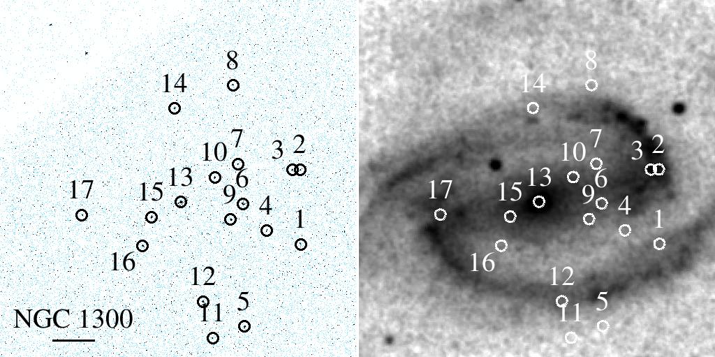
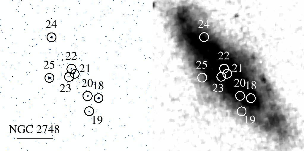
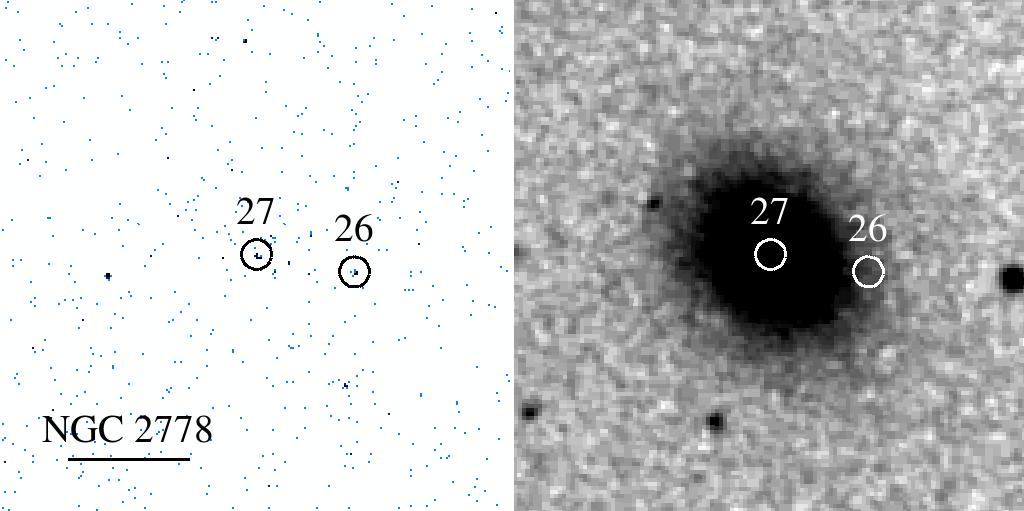
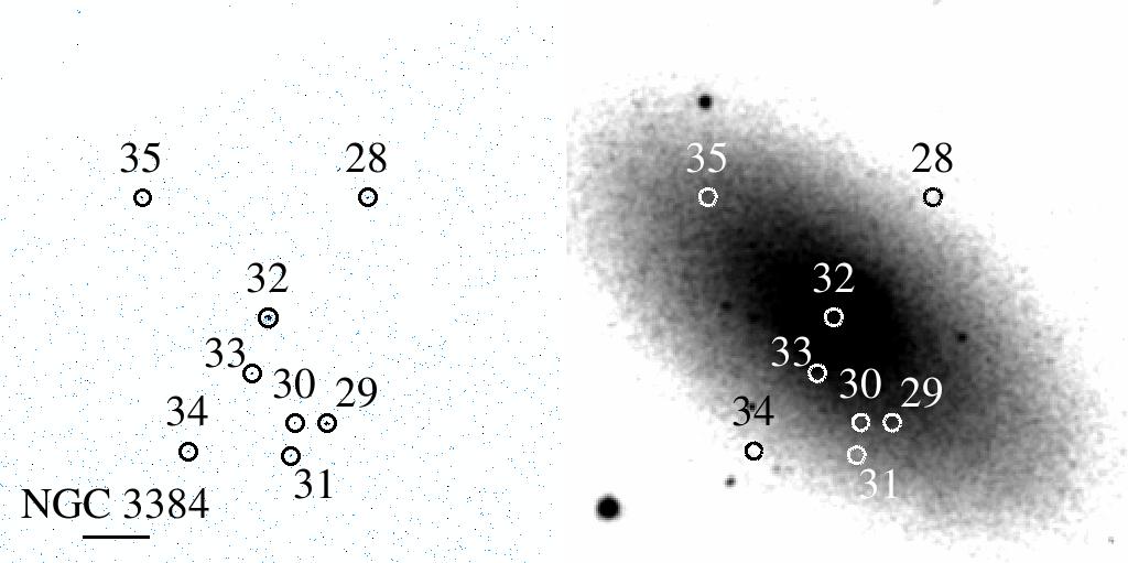
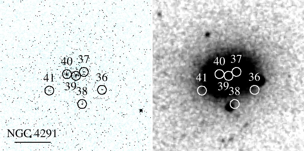
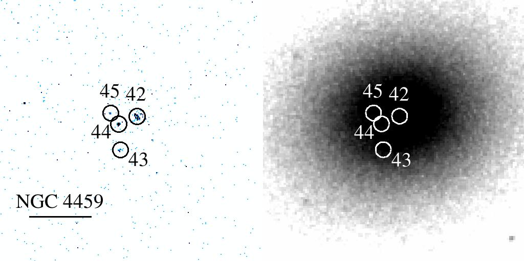
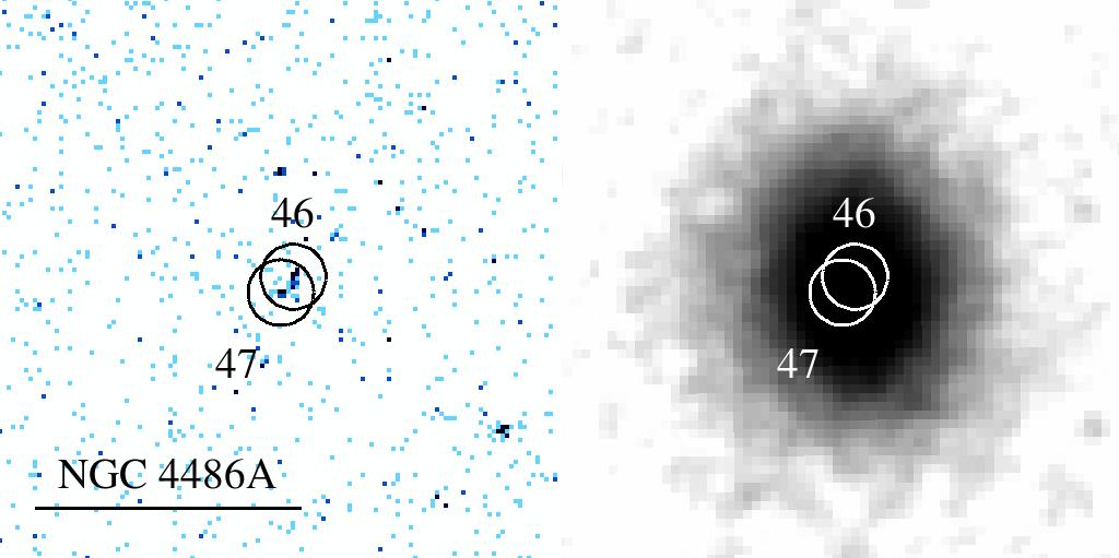
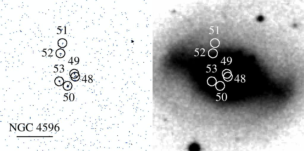
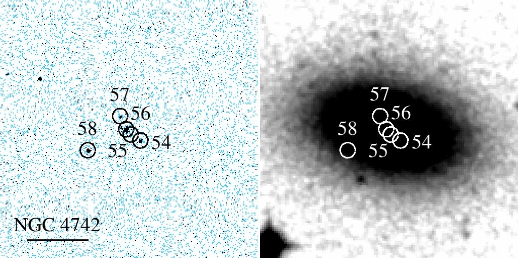
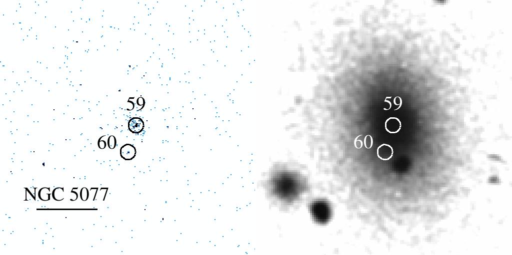
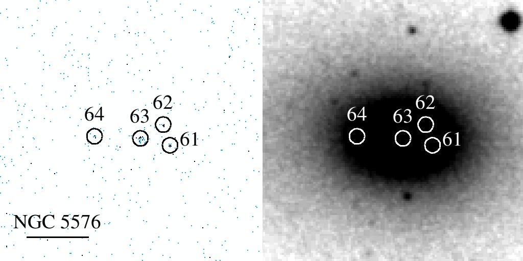
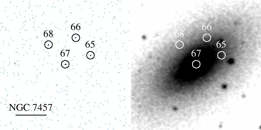
[rgb]0.54,0,0bookmarkcolor imagesimagesFig 1: X-ray and optical images.Fig 1: X-ray and optical images. [rgb]0,0,0bookmarkcolor

2.3. Astrometry

Because we are principally interested in the nuclear X-ray source of each galaxy, we have taken extra care in identifying which point source is the nuclear source. For most galaxies it was unambiguous: there was only one point source consistent with the optical or infrared center of the galaxy. In three galaxies (NGC 4486A, NGC 4596, and NGC 4742) there were two X-ray point sources that were consistent with the position of the galaxy’s center. In a fourth galaxy (NGC 3384), there was faint emission that was not detected by wavdetect as a point source, but which we considered for potential confusion. Typical separation of the confusing sources was 1 to 3″, which requires only modest absolute astrometric corrections. For the four galaxies, we registered the Chandra images to Sloan Digital Sky Survey (SDSS) or Deep Near Infrared Survey (DENIS) coordinates using background AGNs that appeared in both the X-ray and optical/infrared images. Each image had between 3 and 6 sources for registration. The optical/infrared center was obvious in each image so that we could unambiguously determine which source was closer to the galaxy center. In the end, we were able to determine that the Chandra coordinates were sufficient for determining the nuclear sources. The nuclear source in each galaxy is identified in Table 5 in the classification column as “Nuc.”

One possible source of confusion is if an X-ray binary was located at the position of the nuclear center. To estimate this amount of contamination, we adopt the Grimm et al. (2003) universal cumulative luminosity function of high-mass X-ray binaries (HMXBs) in a given galaxy as a function of star formation rate, $\mathrm{SFR}$:

$$N(>L)=5.4(\mathrm{SFR}/{{M}}_{\scriptscriptstyle\odot}\ \mathrm{\ {yr^{-1}}})\left[\left(L/10^{38}\ \mathrm{erg\ s^{-1}}\right)^{-0.61}-0.038\right],$$ (1)

where the second term in the brackets comes from assuming an upper limit of $L_{X}=2.1\times 10^{40}\ \mathrm{erg\ s^{-1}}$ for a HMXB and can be neglected for our calculations. We take the luminsoity of each nuclear source; e.g., for the dimmest source, $L_{X}=3\times 10^{38}\ \mathrm{erg\ s^{-1}}$ so that $N(L>3\times 10^{38}\ \mathrm{erg\ s^{-1}})=2.8(\mathrm{SFR}/{{M}}_{\scriptscriptstyle\odot}\ \mathrm{\ {yr^{-1}}})$. We calculated the star formation rate, $\mathrm{SFR}$, assuming the (Rosa-González et al., 2002) estimator,

$$\mathrm{SFR}=4.5\times 10^{-44}\ {{M}}_{\scriptscriptstyle\odot}\ \mathrm{\ {yr^{-1}}}(L_{\mathrm{FIR}}/\mathrm{erg\ s^{-1}}),$$ (2)

where the far-infrared luminosity is calculated as $L_{\mathrm{FIR}}=1.7\lambda F_{\lambda}$ at $\lambda=60\ \mu\mathrm{m}$. This estimator is based on the Kennicutt (1998) prescritpion and agrees with other, similar prescriptions (e.g., Bell, 2003). Using far-infrared may overestimate the star-formation rate in early-type galaxies but is conservative for our argument. We based our calculations on the the IRAS $60\ \mu\mathrm{m}$ flux density (Knapp et al., 1989) for all galaxies except NGC 5077 for which we substituted the MIPS $70\ \mu\mathrm{m}$ flux density (Temi et al., 2009). The galaxy with the highest star-formation rate in our sample is NGC 2748 with $\mathrm{SFR}=2.0\ {{M}}_{\scriptscriptstyle\odot}\ \mathrm{\ {yr^{-1}}}$, and all but 4 have $\mathrm{SFR}<0.1\ {{M}}_{\scriptscriptstyle\odot}\ \mathrm{\ {yr^{-1}}}$. If we assume that the X-ray binaries follow the light in the galaxy, then we can estimate the number of potential contaminating sources. This is an overestimate of central contamination probability for galaxies like NGC 1300 for which X-ray binaries follow the high rate of star formation in the spiral arms. The starlight in the central 1″, roughly our astrometric uncertainty, ranges from approximately 10% for NGC 1300 to less than 1%. Assuming 10% for all galaxies, we can calculate the expected number of contaminating sources at the center each galaxy. The values range from 0.04 for NGC 2748 to less than 0.01 for the majority. These numbers are conservative because the actual amount of light at the center of each galaxy is less 10%, and the star formation rate may be over-estimated in the early-type galaxies.

For early-type galaxies, a greater concern is the chance positioning of a low-mass X-ray binary (LMXB), which generally traces an older population (Kim & Fabbiano, 2004). In this case, we use the results of Kim & Fabbiano (2004), who found that the cumulative number of LMXBs greater than a luminosity, $L_{X}$ to scale as $N(>L_{X})\sim L_{X}^{-1}$, with a total luminosity of the LMXB population scaling with the galaxy luminosity $L_{K}$ as $L_{\mathrm{pop}}=(0.2\pm 0.08)\times 10^{30}\ \mathrm{erg\ s^{-1}}L_{K}/L_{K{\scriptscriptstyle\odot}}$. This is the most concern for NGC 5077, which has the largest total $K$-band luminosity of $L_{K}=8.5\times 10^{10}\ L_{K{\scriptscriptstyle\odot}}$ (Skrutskie et al., 2006), and for NGC 4486A, which has the lowest nuclear luminosity ($L_{X}=2.5\times 10^{38}\ \mathrm{erg\ s^{-1}}$) and a $K$-band luminosity of $L_{K}=1.5\times 10^{10}\ L_{K{\scriptscriptstyle\odot}}$ (Skrutskie et al., 2006). Again assuming that LMXBs follow the light, the expected number of LMXBs that would be as bright or brighter than the identified nuclear sources is less than 0.005 and 0.04 for NGC 5077 and NGC 4486A, respectively. It is lower for all other galaxies. Because each galaxy type is predominantly affected by contamination from only one of HMXBs or LMXBs and not both, the combined expected contamination by both are then all less than 0.05. Thus we expect not to have incorrectly identified an X-ray binary as an SMBH source.

2.4. Spectral reduction

We followed the standard pipeline in reduction of all data sets, using the most recent Chandra data reduction software package (CIAO version 4.3) and calibration databases (CALDB version 4.4.3). There was no significant background flaring, so there was no need for filtering. We used the CIAO tool psextract to extract the point-source spectra. Since our observations all used the Advanced CCD Imaging Spectrometer (ACIS), we ran psextract with the mkacisrmf tool to create the response matrix file (RMF) and with mkarf set for ACIS ancillary response file (ARF) creation. Source regions were circles with centers at the coordinates given by wavdetect. The radii of the regions were the semimajor axes of the wavdetect error ellipses. This accounts for two effects: (1) the uncertainty in the location of the source and (2) the degradation in the point spread function off axis. For background regions, we used annuli with inner radii just larger than the source region radius and outer radii that was typically 14 pixels larger.

2.5. Spectral fitting

We modeled the reduced spectra using XSPEC12 (Arnaud, 1996). For some sources we used $\chi^{2}$ statistics and for others $C$-stat statistics (Cash, 1979). The decision on which statistics to use was based on the number of photons available for binning in energy bands. If binning the spectra in energy so that each bin contained a minimum of 20 counts resulted in five or more bins, we used $\chi^{2}$ statistics; otherwise we used $C$-stat statistics with unbinned spectra. There is necessarily a loss of information when binning the spectra, but we found when using both types of statistics on sources that had enough counts to support it, the resulting parameter estimates were always consistent within 1$\sigma$. We report the results from $\chi^{2}$ statistics on account of the intuitive nature of the goodness-of-fit with $\chi^{2}$ statistics.

All spectra were modeled with a photoabsorbed power-law model with the intrinsic flux modeled directly as one of the parameters, i.e., the XSPEC model used was phabs(cflux * powerlaw), with the cflux component normalized to the 2–10 keV band. The spectra were fitted from 0.3 to 10 keV. While most of the photon counts above $\sim 7$ keV are probably dominated by background, the fitting methodology takes this into account. We tested our results for sensitivity to the adopted upper energy cutoff and found that as long it was greater than 5 keV, our results were robust in the sense that they changed by far less than the 1$\sigma$ uncertainties. When fitting the spectrum, we set a hard minimum for the absorption to be the Galactic value for $N_{\mathrm{H}}$ towards each source (Bajaja et al., 2005), but in calculating the uncertainty in the column, we allowed it to drop below this value. The results of the spectral fits are presented in Table 2 with best-fit parameters and 1$\sigma$ (68%) uncertainties for $N_{\mathrm{H}}$, $\log F_{2\textrm{--}10}$, and $\Gamma$ (the power-law index). Some sources did not have sufficient counts to produce reliable fits and are not included in the table. Fits to three sources (5, 14, and 62) were unconstrained on at least the spectral index parameter, $\Gamma$, and we consider these fits approximate.

Table 2Results of spectral fits

Galaxy	ID	Class.	$N_{H}$	$\log{F_{2\textrm{--}10}}$	$\Gamma$	$\chi^{2}/\mathrm{d.o.f.}$
(1)	(2)	(3)	(4)	(5)	(6)	(7)
NGC1300	3		$0.0_{-0.0}^{+0.3}$	$-15.0_{-0.5}^{+0.3}$	$2.6_{-0.6}^{+1.6}$	…
…	5		$4.4_{-0.7}^{+0.4}$	$-14.5_{-0.2}^{+0.2}$	$10.0_{\phantom{-0.0}}^{\phantom{+0.0}}$	…
…	6	ULX	$0.6_{-0.2}^{+0.3}$	$-14.6_{-0.2}^{+0.2}$	$4.3_{-0.9}^{+1.1}$	…
…	9	ULX	$0.9_{-0.8}^{+0.9}$	$-15.5_{-0.9}^{+0.5}$	$5.9_{-3.4}^{+4.0}$	…
…	10		$0.1_{-0.1}^{+0.3}$	$-15.0_{-0.6}^{+0.4}$	$2.8_{-0.7}^{+1.7}$	…
…	12	ULX	$0.3_{-0.2}^{+0.3}$	$-15.1_{-0.5}^{+0.4}$	$3.8_{-1.2}^{+1.7}$	…
…	13	Nuc.	$0.0_{-0.0}^{+0.1}$	$-13.0_{-0.1}^{+0.1}$	$0.4_{-0.2}^{+0.3}$	4.51/ 3
…	14		$0.6_{-0.6}^{+0.4}$	$-14.8_{\phantom{-0.0}}^{\phantom{+0.0}}$	$4.1_{\phantom{-0.0}}^{\phantom{+0.0}}$	…
NGC2748	18	ULX	$1.6_{-0.5}^{+0.6}$	$-13.2_{-0.1}^{+0.1}$	$2.3_{-0.7}^{+0.7}$	2.09/ 3
…	20		$0.1_{-0.1}^{+0.2}$	$-14.4_{-0.3}^{+0.2}$	$1.8_{-0.5}^{+0.9}$	…
…	21	Nuc.	$1.0_{-0.5}^{+1.2}$	$-15.0_{-0.6}^{+0.5}$	$5.0_{-2.0}^{+4.1}$	…
…	22	ULX	$1.0_{-0.4}^{+0.6}$	$-15.0_{-0.4}^{+0.3}$	$5.1_{-1.6}^{+2.3}$	…
…	23	ULX	$2.3_{-1.0}^{+1.9}$	$-14.4_{-0.4}^{+0.2}$	$5.1_{-1.7}^{+6.4}$	…
…	24	ULX	$1.6_{-0.3}^{+0.4}$	$-13.5_{-0.1}^{+0.1}$	$3.0_{-0.5}^{+0.5}$	…
…	25	ULX	$0.2_{-0.1}^{+0.1}$	$-13.7_{-0.1}^{+0.1}$	$2.9_{-0.4}^{+0.4}$	6.23/ 9
NGC2778	26	ULX	$0.2_{-0.2}^{+0.2}$	$-14.5_{-0.4}^{+0.3}$	$2.4_{-0.8}^{+1.1}$	…
…	27	Nuc.	$0.2_{-0.2}^{+0.3}$	$-15.7_{-0.8}^{+0.6}$	$4.6_{-1.4}^{+2.6}$	…
NGC3384	29		$0.0_{-0.0}^{+0.2}$	$-13.3_{-0.3}^{+0.2}$	$1.0_{-0.3}^{+0.7}$	…
…	30	ULX	$0.6_{-0.3}^{+0.4}$	$-15.2_{-0.4}^{+0.4}$	$4.1_{-1.4}^{+1.9}$	…
…	32	Nuc.	$0.1_{-0.1}^{+0.2}$	$-13.8_{-0.3}^{+0.2}$	$2.0_{-0.4}^{+0.7}$	…
…	34	ULX	$0.8_{-0.5}^{+0.8}$	$-14.9_{-0.7}^{+0.5}$	$3.8_{-1.8}^{+3.3}$	…
…	35	ULX	$0.3_{-0.2}^{+0.3}$	$-15.2_{-0.4}^{+0.4}$	$4.2_{-1.4}^{+1.8}$	…
NGC4291	36		$0.1_{-0.1}^{+0.3}$	$-14.5_{-0.5}^{+0.3}$	$1.8_{-0.6}^{+1.2}$	…
…	37	ULX	$1.6_{-0.6}^{+1.1}$	$-14.8_{-0.3}^{+0.2}$	$6.1_{-1.7}^{+2.6}$	…
…	38		$0.6_{-0.5}^{+2.2}$	$-14.0_{-0.4}^{+0.3}$	$1.4_{-0.9}^{+2.5}$	…
…	39	Nuc.	$0.1_{-0.1}^{+0.1}$	$-13.9_{-0.1}^{+0.1}$	$1.7_{-0.4}^{+0.4}$	…
…	40	ULX	$0.0_{-0.0}^{+0.1}$	$-13.6_{-0.1}^{+0.1}$	$1.4_{-0.3}^{+0.3}$	1.07/ 3
…	41		$1.1_{-0.7}^{+2.2}$	$-15.6_{-0.7}^{+0.5}$	$6.3_{-2.7}^{+3.7}$	…
NGC4459	42	Nuc.	$0.0_{-0.0}^{+0.1}$	$-13.6_{-0.1}^{+0.1}$	$1.8_{-0.2}^{+0.3}$	4.28/ 4
…	43	ULX	$1.7_{-0.8}^{+0.9}$	$-14.6_{-0.2}^{+0.2}$	$4.7_{-1.7}^{+2.1}$	…
…	44		$0.3_{-0.1}^{+0.2}$	$-13.6_{-0.1}^{+0.1}$	$1.8_{-0.3}^{+0.4}$	…
NGC4486A	46		$0.4_{-0.2}^{+0.3}$	$-14.2_{-0.2}^{+0.2}$	$2.5_{-0.6}^{+0.8}$	…
…	47	Nuc.	$0.3_{-0.3}^{+0.6}$	$-14.4_{-0.3}^{+0.4}$	$2.0_{-1.0}^{+1.4}$	…
NGC4596	48	Nuc.	$0.0_{-0.0}^{+0.2}$	$-14.4_{-0.3}^{+0.2}$	$2.0_{-0.4}^{+0.9}$	…
…	49		$0.0_{-0.0}^{+0.2}$	$-13.9_{-0.2}^{+0.1}$	$1.5_{-0.3}^{+0.6}$	…
…	50		$0.1_{-0.1}^{+0.1}$	$-14.0_{-0.2}^{+0.2}$	$2.0_{-0.5}^{+0.6}$	…
…	53		$0.0_{-0.0}^{+0.0}$	$-13.9_{-0.2}^{+0.1}$	$1.1_{-0.3}^{+0.3}$	…
NGC4742	54		$0.3_{-0.1}^{+0.1}$	$-13.8_{-0.1}^{+0.1}$	$2.2_{-0.4}^{+0.4}$	…
…	55	ULX	$1.1_{-0.5}^{+0.7}$	$-14.5_{-0.5}^{+0.3}$	$3.5_{-1.2}^{+2.4}$	…
…	56	Nuc.	$0.1_{-0.1}^{+0.1}$	$-13.6_{-0.1}^{+0.1}$	$1.7_{-0.2}^{+0.4}$	7.01/ 4
…	57	ULX	$0.4_{-0.3}^{+0.5}$	$-15.4_{-0.6}^{+0.5}$	$4.3_{-1.7}^{+2.6}$	…
…	58		$0.0_{-0.0}^{+0.1}$	$-13.5_{-0.2}^{+0.1}$	$1.3_{-0.3}^{+0.3}$	…
NGC5077	59	Nuc.	$0.0_{-0.0}^{+0.1}$	$-13.5_{-0.1}^{+0.1}$	$1.5_{-0.2}^{+0.2}$	2.18/ 4
…	60		$0.2_{-0.2}^{+0.4}$	$-15.1_{-0.6}^{+0.5}$	$3.1_{-1.2}^{+2.2}$	…
NGC5576	61	ULX	$0.5_{-0.4}^{+0.6}$	$-14.7_{-0.7}^{+0.5}$	$3.0_{-1.4}^{+2.9}$	…
…	62		$4.8_{\phantom{-0.0}}^{\phantom{+0.0}}$	$-14.5_{\phantom{-0.0}}^{\phantom{+0.0}}$	$9.5_{\phantom{-0.0}}^{\phantom{+0.0}}$	…
…	63	Nuc.	$0.5_{-0.2}^{+0.2}$	$-14.5_{-0.3}^{+0.2}$	$3.5_{-0.8}^{+1.1}$	…
…	64	ULX	$0.4_{-0.4}^{+0.6}$	$-15.7_{-0.8}^{+0.9}$	$5.1_{-2.2}^{+2.8}$	…
NGC7457	67	Nuc.	$0.3_{-0.2}^{+0.2}$	$-14.4_{-0.3}^{+0.3}$	$2.5_{-0.8}^{+1.0}$	…
…	68		$0.3_{-0.2}^{+0.3}$	$-14.5_{-0.4}^{+0.3}$	$2.8_{-0.9}^{+1.2}$	…

Note. — This table lists the best-fit parameters with $1\sigma$ uncertainties of our spectral fits to sources with sufficient counts to warrant fitting. If we could not reliably obtain uncertainties, we omit the listing of errors and consider the results approximate. Columns list: (1) the name of the galaxy in which the source appears to lie; (2) our running identification number; (3) classification of source; (4) total absorption column towards the source in units of $10^{22}\ \mathrm{cm^{-2}}$; (5) logarithmic normalization of the powerlaw in unabsorbed (intrinsic) flux in the 2–10 keV band in units of $\mathrm{erg\ s^{-1}\ cm^{-2}}$; (6) powerlaw slope; and (7) $\chi^{2}$ per degrees of freedom if there were sufficient counts to use $\chi^{2}$ statistics.

[rgb]0,0,0.54bookmarkcolor table.0table.0Table 2: Parameters of spectral fitsTable 2: Parameters of spectral fits [rgb]0,0,0bookmarkcolor

3. Analysis and Discussion

3.1. SMBHs

Table 3Nuclear fluxes

Galaxy	ID	$F_{0.3\textrm{--}2}$	$L_{0.3\textrm{--}2}$	$F_{2\textrm{--}10}$	$L_{2\textrm{--}10}$	$F_{0.3\textrm{--}10}$	$L_{0.3\textrm{--}10}$	$\log(L_{2\textrm{--}10}/L_{\mathrm{Edd}})$
(1)	(2)	(3)	(4)	(5)	(6)	(7)	(8)	(9)
NGC1300	13	$7.3^{+0.2}_{-2.5}\times 10^{-15}$	$3.8^{+1.1}_{-0.5}\times 10^{38}$	$1.1^{+0.4}_{-0.3}\times 10^{-13}$	$5.2^{+1.2}_{-1.1}\times 10^{39}$	$1.1^{+0.3}_{-0.3}\times 10^{-13}$	$5.6^{+1.2}_{-1.1}\times 10^{39}$	$-6.3\pm 0.3$
NGC2748	21	$2.0^{+0.4}_{-1.1}\times 10^{-15}$	$1.9^{+2599.2}_{-1.8}\times 10^{40}$	$7.3^{+27.5}_{-6.0}\times 10^{-16}$	$6.9^{+12.5}_{-4.9}\times 10^{37}$	$2.7^{+0.8}_{-1.3}\times 10^{-15}$	$2.0^{+694.8}_{-1.8}\times 10^{40}$	$-8.0\pm 0.7$
NGC2778	27	$4.3^{+1.1}_{-4.2}\times 10^{-15}$	$1.9^{+49.2}_{-1.5}\times 10^{39}$	$1.9^{+68.9}_{-1.8}\times 10^{-16}$	$1.4^{+4.0}_{-1.1}\times 10^{37}$	$4.4^{+1.0}_{-4.3}\times 10^{-15}$	$1.9^{+49.2}_{-1.5}\times 10^{39}$	$-8.2\pm 0.8$
NGC3384	32	$1.3^{+0.1}_{-0.4}\times 10^{-14}$	$3.2^{+3.4}_{-0.9}\times 10^{38}$	$1.7^{+1.5}_{-0.8}\times 10^{-14}$	$2.8^{+1.7}_{-1.2}\times 10^{38}$	$3.0^{+0.5}_{-1.1}\times 10^{-14}$	$5.9^{+2.4}_{-0.9}\times 10^{38}$	$-6.9\pm 0.2$
NGC4291	39	$5.6^{+0.7}_{-1.6}\times 10^{-15}$	$6.6^{+4.2}_{-2.2}\times 10^{38}$	$1.4^{+0.6}_{-0.4}\times 10^{-14}$	$1.0^{+0.4}_{-0.3}\times 10^{39}$	$1.9^{+0.3}_{-0.5}\times 10^{-14}$	$1.7^{+0.3}_{-0.3}\times 10^{39}$	$-7.6\pm 0.4$
NGC4459	42	$1.6^{+0.1}_{-0.6}\times 10^{-14}$	$6.3^{+1.8}_{-0.8}\times 10^{38}$	$2.3^{+0.9}_{-0.7}\times 10^{-14}$	$8.0^{+2.2}_{-2.0}\times 10^{38}$	$3.9^{+0.3}_{-1.4}\times 10^{-14}$	$1.4^{+0.2}_{-0.2}\times 10^{39}$	$-7.1\pm 0.1$
NGC4486A	47	$1.8^{+0.4}_{-0.6}\times 10^{-15}$	$1.3^{+11.5}_{-0.8}\times 10^{38}$	$4.0^{+4.3}_{-2.4}\times 10^{-15}$	$1.4^{+1.6}_{-0.8}\times 10^{38}$	$5.8^{+2.4}_{-3.5}\times 10^{-15}$	$2.8^{+10.5}_{-0.9}\times 10^{38}$	$-7.1\pm 0.4$
NGC4596	48	$4.2^{+0.7}_{-2.9}\times 10^{-15}$	$1.8^{+2.4}_{-0.4}\times 10^{38}$	$3.9^{+4.3}_{-2.2}\times 10^{-15}$	$1.5^{+1.0}_{-0.8}\times 10^{38}$	$8.1^{+0.3}_{-5.1}\times 10^{-15}$	$3.3^{+1.7}_{-0.7}\times 10^{38}$	$-7.9\pm 0.3$
NGC4742	56	$1.3^{+0.1}_{-0.3}\times 10^{-14}$	$5.2^{+2.3}_{-1.0}\times 10^{38}$	$2.5^{+0.8}_{-0.6}\times 10^{-14}$	$7.2^{+2.0}_{-1.9}\times 10^{38}$	$3.8^{+0.5}_{-0.8}\times 10^{-14}$	$1.2^{+0.2}_{-0.2}\times 10^{39}$	$-6.4\pm 0.2$
NGC5077	59	$1.3^{+0.1}_{-0.5}\times 10^{-14}$	$3.6^{+0.9}_{-0.5}\times 10^{39}$	$2.8^{+0.9}_{-0.7}\times 10^{-14}$	$6.8^{+1.6}_{-1.5}\times 10^{39}$	$4.1^{+0.4}_{-1.2}\times 10^{-14}$	$1.0^{+0.2}_{-0.1}\times 10^{40}$	$-7.2\pm 0.2$
NGC5576	63	$4.7^{+0.5}_{-2.1}\times 10^{-15}$	$4.3^{+14.5}_{-2.8}\times 10^{39}$	$2.7^{+5.6}_{-1.8}\times 10^{-15}$	$2.6^{+1.9}_{-1.3}\times 10^{38}$	$7.4^{+1.1}_{-4.7}\times 10^{-15}$	$4.6^{+15.4}_{-2.7}\times 10^{39}$	$-8.0\pm 0.3$
NGC7457	67	$3.9^{+0.1}_{-2.4}\times 10^{-15}$	$3.1^{+7.7}_{-1.8}\times 10^{38}$	$4.3^{+16.0}_{-3.4}\times 10^{-15}$	$1.0^{+0.9}_{-0.5}\times 10^{38}$	$8.2^{+1.4}_{-6.1}\times 10^{-15}$	$4.2^{+6.8}_{-1.5}\times 10^{38}$	$-6.7\pm 0.3$

Note. — Fluxes and luminosities of nuclear sources, assumed to be the SMBH in each galaxy. For each source, we list the $F$, the absorbed (apparent) flux in units of $\mathrm{erg\ s^{-1}\ cm^{-2}}$, and $L$, the unabsorbed (intrinsic) luminosity in units of $\mathrm{erg\ s^{-1}}$, for each of the 0.3–2, 2–10, and 0.3–10 bands. Uncertainties are listed as 1$\sigma$ intervals, and the final column includes uncertainties in the mass. Note that because of covariances between the model parameters, the full band is not simply the sum of the soft and hard bands with uncertainties added in quadruture. The final column lists the logarithmic Eddington fraction. While some of the sources have full-band luminosities consistent with zero at about the 3$\sigma$ level, point sources at the centers of each galaxy at greater than 4$\sigma$ confidence. This is because the luminosity depends upon an unknown spectral form whereas detection depends on raw count rate above the background. For example, the full-band luminosity for source 27 in NGC 2778 is only about 1$\sigma$ above zero, but inspection of Table 5 shows that the net count rate for this source in the full band (summing uncertainties in quadruture) is $(9.6\pm 2.1)\times 10^{-4}\ \mathrm{\ {ctss^{-1}}}$.

[rgb]0,0,0.54bookmarkcolor table.0table.0Table 3: Fluxes and luminosities of nuclear sourcesTable 3: Fluxes and luminosities of nuclear sources [rgb]0,0,0bookmarkcolor

The primary scientific goal of our Chandra program is to measure the luminosities of SMBHs with direct, primary mass measurements. For each nuclear source we list the flux and luminosity (assuming isotropic radiation and the distance to each galaxy listed in Table 2.1) for the 0.3–2, 2–10, and 0.3–10 keV bands in Table 3. The fluxes listed are intrinsic (unabsorbed). Note that the fluxes in each band are derived from fits to the X-ray spectrum using different bands as normalizations, and, therefore, the uncertainties are correlated. In Figure 6 (and 7), we show plots of the spectra of the nuclear sources in all 12 galaxies, along with the best-fit model spectrum for each source. The parameters of the best-fit model spectra are in Table 2. The spectra have been binned for visualization purposes. The spectra are all well fit by a power law, and none of the spectra requires a more complicated model.

Figure 2 is a histogram we call a “distributed histogram” of the values of the power-law exponent ($\Gamma$) inferred from our spectral fits. The uncertainties in $\Gamma$ in some spectral fits are much larger than some of the others and in some cases much larger than the size of the histogram bins in which we are interested. To account for this we assume that the errors in $\Gamma$ are distributed normally and plot the contribution to each bin according to the value and error. That is, for each value of $\Gamma$, the histogram in a bin of width $w$ that is $x\sigma$ away from the central value is $w(\sigma\sqrt{2\pi})^{-1}\exp(-x^{2}/2)$, where $\sigma$ is the error of the measurement. We also include analogous data from Gültekin et al. (2009a). There is an obvious peak at $\Gamma\approx 2$. Related to the distributed histogram we introduce a “distributed median,” which we define as the point at which the area under the distributed histogram is half of the total area. The distributed median of $\Gamma$ is 1.86, very close to the canonical 1.7 power-law for AGNs (e.g., Mushotzky, 1984).

Figure 2.— Distributed histogram of values of $\Gamma$, the slope of the power-law. This is a histogram of the values of $\Gamma$ inferred from our spectral fits, with each value spread out among the bins according to the error on the value, assuming a normal distribution. That is, for each value of $\Gamma$, the histogram in a bin of width $w$ that is $x\sigma$ away from the central value is $w(\sigma\sqrt{2\pi})^{-1}\exp(-x^{2}/2)$, where $\sigma$ is the error of the measurement. This method of visualizing the histogram is useful when the errors vary in magnitude from one measurement to the next and when the errors are larger than the size of an interesting histogram bin. The new data from this paper are in red, and the new results plus those from Gültekin et al. (2009a) are in gray. The point that divides the area under the distributed histogram in two is $\Gamma=1.86$, very close to the canonical $\Gamma=1.7$ power-law in AGNs (Mushotzky, 1984).

[rgb]0.54,0,0bookmarkcolor gammahistgammahistFig 2: Histogram of Gamma.Fig 2: Histogram of Gamma. [rgb]0,0,0bookmarkcolor

Because we have direct, primary measurements of the mass of the central black hole in each of these galaxies, we can report luminosities as true Eddington fractions. In Figure 3, we plot a distributed histogram of $\log(L_{2\textrm{--}10}/L_{\mathrm{Edd}})$. We include uncertainties in the black hole mass but instead assume the value given in Table 2.1. As can be seen in the figure, the hard X-ray Eddington fractions are small, in the range $10^{-8}<L_{2\textrm{--}10}/L_{\mathrm{Edd}}<10^{-6}$, and the distributed median of the logarithmic Eddington fraction is $-7.2$. The reason that all sources are at such low accretion rates is that the sources were selected based on having a dynamical mass measurement of the central black hole. Most of the black hole masses in Gültekin et al. (2009c) are based on stellar dynamical models (e.g., Gültekin et al., 2009b) and gas dynamical models (e.g., Barth et al., 2001), and these methods are best when the there is no contamination from AGN light. Typical bolometric corrections for low-luminosity sources such as these is $\sim 10$ (Vasudevan & Fabian, 2007), so that the bolometric Eddington fractions of these sources are in the range $10^{-7}$–$10^{-5}$.

Note that the power of using dynamical mass measurements instead of secondary mass estimates is evident in our tabulation of $L_{2\textrm{--}10}/L_{\mathrm{Edd}}$ values. The median error in $\log(L_{2\textrm{--}10})$ is 0.25 dex, the median error in $\log M_{\mathrm{BH}}$ is 0.17 dex, and the median error in secondary mass estimates is 0.51 dex. Thus the uncertainty in secondary mass estimates dominates the total uncertainty in $\log f_{\mathrm{Edd}}$ and is completely subdominant when using primary measurements.

Figure 3.— Distributed histogram of values of $\log(L_{2\textrm{--}10}/L_{\mathrm{Edd}})$, the slope of the power-law. This is a histogram of the values of $L_{2\textrm{--}10}/L_{\mathrm{Edd}}$ inferred from our spectral fits, with each value spread out among the bins according to the error on the value, assuming a normal distribution. That is, for each value of $\log(L_{2\textrm{--}10}/L_{\mathrm{Edd}})$ with measurement error $\sigma$, the histogram in a bin of width $w$ that is $x\sigma$ away from the central value is $w(\sigma\sqrt{2\pi})^{-1}\exp(-x^{2}/2)$. This method of visualizing the histogram is useful when the errors vary in magnitude from one measurement to the next and when the errors are larger than the size of an interesting histogram bin. The distributed histogram shows that the accretion rates that we study in this sample are very low.

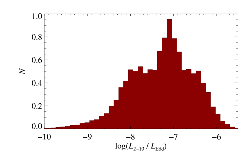
[rgb]0.54,0,0bookmarkcolor feddhistfeddhistFig 3: Histogram of X-ray Eddington fraction.Fig 3: Histogram of X-ray Eddington fraction. [rgb]0,0,0bookmarkcolor

In Figure 4 we plot the spectral power-law slope as a function of $\log(L_{2\textrm{--}10}/L_{\mathrm{Edd}})$ for the current data and for the data in Gültekin et al. (2009a). We also fit for a linear relation between these two quantities. There is one source, Cen A, with $L_{2\textrm{--}10}/L_{\mathrm{Edd}}>10^{-3}$ and $\Gamma<0$, that is likely Compton thick so that a power-law index at energies below 10 keV possibly probes different energetics and/or accretion physics than the rest of the sources. Because of this and the potential lever arm it could have on the fit, we fit both with and without this source, but it had no effect on our results. Since there is a strong covariance between $\Gamma$ and $L_{2\textrm{--}10}$, we do not include measurement uncertainties on $L_{2\textrm{--}10}$ but instead bootstrap (resample with replacement) the sample to estimate uncertainties, expressing our result as the median with 68% interval. A histogram of the bootstrap results showed roughly Gaussian distributions, indicating reliability of results. Finally we include a scatter term, assumed normally distributed in $\Gamma$ because the data clearly deviate from any single line by more than their measurement uncertainties. The fitting method and code are the same as that used and described in Gültekin et al. (2009c). The method uses a generalized maximum likelihood method that is capable of including upper limits, arbitrary error distributions, and arbitrary form of intrinsic scatter. Here we assume Gaussian errors in $\Gamma$ and Gaussian scatter in the $\Gamma$ direction. We plot the best-fit linear relation, which is $\Gamma=1.8\pm 0.2-(0.24\pm 0.12)\log(L_{2\textrm{--}10}/10^{-7}L_{\mathrm{Edd}})$ with an rms intrinsic scatter of $0.65\pm 0.20$ (uncertainties are 1$\sigma$ here and throughout this paper). Our results are inconsistent with a slope of zero or larger at the 2$\sigma$ level.

To illustrate what the additional data in this program add as well as how sensitive these results are to the use of dynamical masses, we perform two exercises. First, we repeat the fit without the new data, yielding a slope of $-0.33\pm 0.25$. So while this is consistent with our full results, it is far less conclusive as to whether the X-ray spectral properties at very low Eddington rates is different from those at high Eddington rates. Second, we fit with the full sample but with masses and uncertainties generated from the $M$–$\sigma$ relation:

$$\log(M_{\mathrm{BH}}/{{M}}_{\scriptscriptstyle\odot})=\alpha+\beta\log(\sigma/200\ \mathrm{km\ s^{-1}}),$$ (3)

where $\sigma$ is the velocity dispersion of the host galaxy, and $\alpha=8.12\pm 0.08$ and $\beta=4.24\pm 0.41$ are the best-fit $M$–$\sigma$ parameters (Gültekin et al., 2009c). Propagating uncertainties, $\epsilon_{x}$, for each quantity, $x$, the variance in logarithmic mass due to random errors is

$$\epsilon_{\log M_{\mathrm{BH}}}^{2}=\epsilon_{\alpha}^{2}+\left[\log\left(\sigma/200\ \mathrm{km\ s^{-1}}\right)\right]^{2}\epsilon_{\beta}^{2}+\frac{\beta^{2}}{\sigma^{2}}\epsilon_{\sigma}^{2}+\epsilon_{0}^{2},$$ (4)

where $\epsilon_{0}=0.44$ is the observed intrinsic scatter in the $M$–$\sigma$ relation. When fitting with these new masses and uncertainties, the slope is $-0.27\pm 0.13$. So it appears that without direct masses, we would have come to the same conclusion, though by using masses derived from the $M$–$\sigma$ relation for the very galaxies from which $M$–$\sigma$ was derived, we necessarily underestimate the amount of systematic errors introduced from using a secondary quantity.

As mentioned in section 2.1, one consequence of our sample selection is that we only cover SMBHs emitting at very low Eddington rates. A direct consequence of this is that our X-ray observations are more susceptible to contamination from a fixed amount of hot gas than would be an X-ray source that was intrinsically brighter. Since hot gas emission typically peaks at an energy below 1 keV, any contamination hot gas in our spectral data would tend to make the spectrum softer and thus we would infer a larger value for $\Gamma$. This is particularly concerning since our results indicate larger values of $\Gamma$ at lower Eddington rates, as this selection effect and contamination would manifest. We have mitigated this as much as possible with our selection of background regions, which are annuli that surround the source regions. This effectively removes the contribution of hot gas that is seen in the background region. If, however, the diffuse emission is more centrally concentrated than the background annulus, then there will still be some contamination from diffuse gas. To take this into account we refit all nuclear sources with an additional astrophysical plasma emission code (APEC Smith et al., 2001) component (with abundance fixed to solar). For all but three the results for $L_{2\textrm{--}10}$ and $\Gamma$ are consistent at the 1$\sigma$ or better, and the remaining 3 are consistent at about the 2$\sigma$ level. This lack of significant change strongly suggests that our results are not affected by the contamination of diffuse gas.

Figure 4.— Slope of the spectral power-law ($\Gamma$) as a function of hard X-ray Eddington fraction ($L_{2\textrm{--}10}/L_{\mathrm{Edd}}$). Large red circles are new results from this paper, and small gray squares are results from Gültekin et al. (2009a). The slope of the best-fit relation to these two data sets, which is drawn as a solid black line, is $0.24\pm 0.12$. The dark shaded region shows the 1$\sigma$ confidence band, and the light shaded region shows the 1$\sigma$ confidence band plus the rms intrinsic scatter. Error bars on each point are 1$\sigma$ uncertainties. For reference we show similar data based primarily on secondary mass estimates from Gu & Cao (2009), Shemmer et al. (2008), Winter et al. (2009), and Younes et al. (2011) as indicated in the legend drawn as small open triangles.

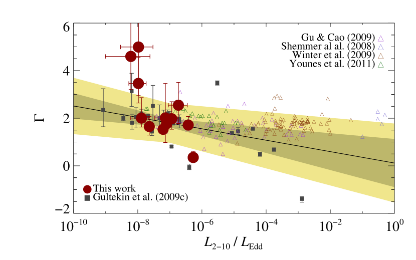
[rgb]0.54,0,0bookmarkcolor gammavsfeddgammavsfeddFig 4: Gamma vs. hard X-ray Eddington fraction.Fig 4: Gamma vs. hard X-ray Eddington fraction. [rgb]0,0,0bookmarkcolor

Our results are consistent with previous works looking at the anti-correlation between $\Gamma$ and Eddington fraction. Using a sample of 55 LLAGNs with a mixture of primary and secondary black-hole-mass measurements, Gu & Cao (2009) fit a linear relation assuming a constant $L_{\mathrm{Bol}}/L_{2\textrm{--}10}=30$. For $L_{\mathrm{Bol}}/L_{\mathrm{Edd}}<10^{-1}$, they inferred $\Gamma=1.55\pm 0.07-(0.09\pm 0.03)\log(L_{\mathrm{Bol}}/L_{\mathrm{Edd}})$. Note that the differences in intercepts between the fits are all a result of defining the independent variable differently. While their results are consistent with ours at about the 1.2$\sigma$ level, the absence of a scatter term in the fitting function may skew the results since the residuals are larger than would be expected just from measurement errors. As part of the Chandra Multiwavelength Project, Constantin et al. (2009) studied 107 LLAGNs with Chandra observations. They found a strong anticorrelation between $\Gamma$ and $L_{\mathrm{Bol}}/L_{\mathrm{Edd}}$, where they assumed $L_{\mathrm{Bol}}=16L_{2\textrm{--}10}$ and used the $M$–$\sigma$ relation to estimate black hole masses. Their Spearman rank correlation coefficient was $-0.75$, and their fit to the relation was $\Gamma=0.98\pm 0.13-(0.27\pm 0.04)\log(L_{\mathrm{Bol}}/L_{\mathrm{Edd}})$. The goodness-of-fit, however, was $\chi^{2}=274$ for 105 degrees of freedom, indicating that it was very unlikely that the data could come from a scatter-free model. In a study of 153 AGNs detected by the Swift Burst Alert Telescope hard X-ray instrument, Winter et al. (2009) found a no correlation between $\Gamma$ and $L_{2\textrm{--}10}/L_{\mathrm{Edd}}$. It is possible that their sample, which is primarily at $L_{2\textrm{--}10}/L_{\mathrm{Edd}}>10^{-4}$ and reaches up to $L_{2\textrm{--}10}/L_{\mathrm{Edd}}\approx 0.04$ is actually measuring an energetically different mode of accretion than our sample. In any case, our study agrees with Winter et al. (2009) that the spectra do not harden with increasing accretion rates. In a study of 13 LINERs with XMM-Newton and/or Chandra observations and assuming very different $M$–$\sigma$ relation (due to Graham et al., 2011), Younes et al. (2011) found $\Gamma=0.11\pm 0.40-(0.31\pm 0.06)\log(L_{2\textrm{--}10}/L_{\mathrm{Edd}})$. A similar anti-correlation is suggested in X-ray binary data (Corbel et al., 2006). Given the difference in assumptions and fitting techniques, we consider all of these results consistent with each other in the following conclusions: (1) there is an anti-correlation between the hard X-ray photon index, $\Gamma$, and Eddington fraction for LLAGNs, and (2) the correlation between $\Gamma$ and $\log(L_{2\textrm{--}10}/L_{\mathrm{Edd}})$ has a slope of roughly $-0.2$.

The anticorrelation between $\Gamma$ and $L_{2\textrm{--}10}/L_{\mathrm{Edd}}$ is in contrast to AGNs emitting at higher Eddington fractions. For example, Shemmer et al. (2008) found from fits to a sample of 35 radio quiet, luminous, and high-Eddington-fraction ($L_{\mathrm{Bol}}/L_{\mathrm{Edd}}\sim 0.01$–1) AGNs that there was a strong positive correlation. From their fits, they found $\log(L_{\mathrm{Bol}}/L_{\mathrm{Edd}})=-2.4\pm 0.6+(0.9\pm 0.3)\Gamma$, corresponding to $\Gamma=2.6+1.1(L_{\mathrm{Bol}}/L_{\mathrm{Edd}})$. Thus our evidence leads us to conclude that we are seeing a change in the physical processes responsible for emission at low Eddington rates.

The softening of the spectrum with decreasing Eddington fractions at low mass accretion rates as we find in our sample is predicted by advection dominated accretion flow (ADAF) models in stellar-mass X-ray binaries (Esin et al., 1997), which should reasonably translate to the low accretion rates seen in our SMBH sources. Esin et al. (1997) models predict a steepening of the 1–10 keV band index of $\Gamma\approx 1.7$ to about 2.2 over mass accretion rates of $\log(\dot{m})=-2.5$ to $-4$, or a slope of approximately 0.33. The comparison is not direct, but our results are fully consistent with this prediction, which is attributed to the fact that at lower accretion rates bremsstrahlung emission becomes relatively more important compared to Comptonizaion.

3.2. ULXs

Ultraluminous X-ray sources (ULXs) are a category of X-ray emitting point sources that are too bright to be explained by isotropic emission resulting from sub-Eddington accretion onto stellar-mass ($M\lesssim 10\ {{M}}_{\scriptscriptstyle\odot}$) black holes and are also non-nuclear so that they are unlikely to be the galaxy’s central SMBH. ULXs are an intriguing class of source because if (1) they are emitting roughly isotropically (i.e., not strongly beamed towards our line of sight), so that we may correctly infer their luminosity, and (2) they are not accreting well above the Eddington limit, so that we may robustly infer a lower limit to the mass, then the most natural explanation is a black hole of mass $\sim 10^{2}$–$10^{5}\ {{M}}_{\scriptscriptstyle\odot}$. These intermediate-mass black holes (IMBHs) would fill the gap in mass between stellar-mass black holes and SMBHs. IMBHs are interesting because their formation in the local universe requires a non-standard path (Miller & Hamilton, 2002; Gültekin et al., 2004, 2006; Portegies Zwart et al., 2004). There are alternative interpretations to ULXs other than IMBHs, including beamed, non-isotropic emission (King et al., 2001). This would change the luminosity inferred from the flux so that it is consistent with sub-Eddington accretion onto stellar-mass black holes. There are at least a few sources (Kaaret et al., 2004; Pakull & Mirioni, 2001) where emission from the surrounding medium argues in favor of roughly isotropic emission. Another alternative is to have super-Eddington accretion, which has been invoked in a number of different ways (Begelman, 2002, 2006). The very bright source ESO 243-49 HLX-1 is similarly difficult to interpret without invoking an IMBH (Farrell et al., 2009).

Table 4Ultraluminous X-ray Source Candidates

Galaxy	ID	$L_{0.3\textrm{--}10}$	$P(L>L_{\mathrm{ULX}})$	$L_{F}$	$p$	$\langle N_{\mathrm{BG}}\rangle$
(1)	(2)	(3)	(4)	(5)	(5)	(6)
NGC1300	6	$8.9^{+40.0}_{-6.0}\times 10^{39}$	$0.92$	$7.8^{+1.3}_{-1.1}\times 10^{38}$	$0.07$	$0.13$
…	9	$2.8^{+1621.1}_{-2.8}\times 10^{40}$	$0.50$	$2.3^{+0.9}_{-0.7}\times 10^{38}$	$0.83$	$0.13$
…	12	$1.5^{+14.2}_{-1.1}\times 10^{39}$	$0.43$	$3.5^{+0.8}_{-0.7}\times 10^{38}$	$0.74$	$0.13$
NGC2748	18	$1.4^{+2.0}_{-0.5}\times 10^{40}$	$>0.99$	$7.0^{+1.1}_{-0.9}\times 10^{39}$	$0.002$	$0.02$
…	22	$2.8^{+101.3}_{-2.5}\times 10^{40}$	$0.88$	$5.2^{+2.0}_{-1.4}\times 10^{38}$	$0.05$	$0.02$
…	23	$9.2^{+1490.0}_{-8.8}\times 10^{40}$	$0.91$	$7.3^{+3.2}_{-2.4}\times 10^{38}$	$0.03$	$0.02$
…	24	$1.9^{+2.3}_{-0.9}\times 10^{40}$	$>0.99$	$4.6^{+0.8}_{-0.7}\times 10^{39}$	$0.002$	$0.02$
…	25	$1.0^{+0.6}_{-0.3}\times 10^{40}$	$>0.99$	$5.8^{+0.4}_{-0.4}\times 10^{39}$	$0.002$	$0.02$
NGC2778	26	$8.0^{+12.5}_{-2.8}\times 10^{38}$	$0.16$	$6.3^{+2.1}_{-1.5}\times 10^{38}$	$0.79$	$0.01$
NGC3384	30	$5.7^{+94.9}_{-4.7}\times 10^{38}$	$0.31$	$6.0^{+2.1}_{-1.6}\times 10^{37}$	$0.16$	$0.03$
…	34	$5.6^{+498.0}_{-4.5}\times 10^{38}$	$0.37$	$9.4^{+6.1}_{-3.9}\times 10^{37}$	$0.39$	$0.03$
…	35	$7.0^{+88.5}_{-5.4}\times 10^{38}$	$0.33$	$1.3^{+0.3}_{-0.3}\times 10^{38}$	$0.49$	$0.03$
NGC4291	37	$2.9^{+15.9}_{-2.7}\times 10^{41}$	$0.99$	$7.8^{+1.9}_{-1.6}\times 10^{38}$	$0.008$	$0.01$
…	40	$2.8^{+0.6}_{-0.5}\times 10^{39}$	$0.96$	$2.5^{+0.4}_{-0.4}\times 10^{39}$	$0.60$	$0.01$
NGC4459	43	$1.7^{+73.0}_{-1.6}\times 10^{40}$	$0.77$	$3.3^{+1.3}_{-1.0}\times 10^{38}$	$0.03$	$0.01$
NGC4596	52	$1.5^{+34.1}_{-1.5}\times 10^{41}$	$0.85$	$2.4^{+0.9}_{-0.6}\times 10^{38}$	$0.27$	$0.01$
NGC4742	55	$1.6^{+53.0}_{-1.2}\times 10^{39}$	$0.46$	$2.5^{+1.2}_{-0.9}\times 10^{38}$	$0.16$	$0.00$
…	57	$9.6^{+419.3}_{-8.2}\times 10^{38}$	$0.41$	$1.3^{+0.5}_{-0.3}\times 10^{38}$	$0.72$	$0.00$
NGC5576	61	$1.3^{+51.6}_{-0.8}\times 10^{39}$	$0.42$	$5.7^{+4.6}_{-2.5}\times 10^{38}$	$0.57$	$0.03$
…	64	$5.9^{+759.1}_{-5.3}\times 10^{39}$	$0.63$	$4.5^{+2.0}_{-1.2}\times 10^{38}$	$0.70$	$0.03$

Note. — A listing of the ULX candidates identified in this survey. Columns list: (1) the name of the galaxy in which the source appears to lie; (2) our running identification number; (3) the unabsorbed (intrinsic) luminosity in the 0.3–10 keV band; (4) the probability, based on the flux parameter uncertainty, that the given source’s luminosity is above the definition of a ULX ($L_{0.3\textrm{--}10}>2\times 10^{39}\mathrm{\ erg\ s^{-1}}$); (5) the 0.3–10 keV luminosity inferred when fixing the absorption column to the Galactic value towards that source; (6) the $p$-value result of our simulations to calculate the significance of the improvement of including $N_{H}$ as a free parameter; and (7) the expected number of background sources in the galaxy with fluxes $F_{0.5\textrm{--}2}>2\times 10^{39}\mathrm{\ erg\ s^{-1}}(4\pi D^{2})^{-1}$. The probability of having at least one background source in the galaxy of such flux is $1-\exp(-\langle N_{\mathrm{BG}}\rangle)\sim\langle N_{\mathrm{BG}}\rangle$. All uncertainties are listed as 1$\sigma$ intervals.

[rgb]0,0,0.54bookmarkcolor table.0table.0Table 4: ULX candidatesTable 4: ULX candidates [rgb]0,0,0bookmarkcolor

Although our survey was not targeted at ULXs, we are sensitive to them and present a list of ULX candidates in table 4. We adopt the definition of (Irwin et al., 2003) that ULXs are sources with $L_{0.3\textrm{--}10}>L_{\mathrm{ULX}}\equiv 2\times 10^{39}\ \mathrm{erg\ s^{-1}}$, which avoids contamination from bright, massive stellar-mass X-ray binaries. We assume that all sources are isotropically emitting at the distance of the host galaxy. Because of measurement uncertainties, there is always a finite probability that a source that appears to have $L_{0.3\textrm{--}10}>L_{\mathrm{ULX}}$, is actually intrinsically too dim to be a ULX. Additionally, sources that are just below $L_{\mathrm{ULX}}$ are still viable ULX candidates. For these reasons, we list all sources that are at least 1$\sigma$ consistent with being a ULX and list $P(L_{0.3\textrm{--}10}>L_{\mathrm{ULX}})$, the probability of the source having $L_{0.3\textrm{--}10}>L_{\mathrm{ULX}}$. This is calculated by finding $\Delta C$, the change in fit statistic, when setting $F_{0.3\textrm{--}10}=2\times 10^{39}\ \mathrm{erg\ s^{-1}}\ (4\pi D^{2})^{-1}$ and refitting. Then we calculate $P(L_{0.3\textrm{--}10}>L_{\mathrm{ULX}})=0.5\pm 0.5\;\mathrm{erf}\;\left[\left(\Delta C/2\right)^{0.5}\right]$, taking the top and bottom sign for when the best-fit luminosity is above or below $L_{\mathrm{ULX}}$, respectively.

One source of contamination is background AGNs that appear to be in the galaxy. We have checked the catalog of Véron-Cetty & Véron (2010) and found no known AGNs at the locations of our ULX candidates, but it is clearly possible for a previously unknown AGN to be located at this position. To quantify this effect, we calculate $\langle N_{\mathrm{BG}}\rangle$, the expected number of background AGNs in the region of the galaxy target with fluxes greater than $2\times 10^{39}\ \mathrm{erg\ s^{-1}}\ (4\pi D^{2})^{-1}$. To do this we use the fits to the background AGN density as a function of flux from (Giacconi et al., 2001). Unfortunately, they only provide fits for fluxes in the 0.5–2 and 2–10 keV bands. Since most of the flux in a power-law source comes from the soft band, we use the softer band and assume that all of the flux comes from this band. Since the relations are approximately linear, if only half of the emission comes from this portion of the band, then the average number of background sources would roughly double, still a small number. It is important to use the whole area of the galaxy and the smallest possible flux for the calculation of $\langle N_{\mathrm{BG}}\rangle$ because we would have listed any source above the threshold flux apparently within the galaxy as a ULX candidate. The expected background for each galaxy is listed in Table 4, and it is small. The probability of a galaxy having at least one confusing background source is $1-\exp(-\langle N_{\mathrm{BG}}\rangle)$, and a lower limit for the probability of an individual ULX candidate’s truly being a ULX is $P(\mathrm{ULX})=P(L_{0.3\textrm{--}10}>L_{\mathrm{ULX}})\exp(-\langle N_{\mathrm{BG}}\rangle)$.

Note that the probability of ULX luminosity that we calculate is only accurate if our spectral model is a reasonably good model. In Figure 8 we plot spectra of the six sources (6, 18, 23, 24, 25, and 40) with $P(L_{0.3\textrm{--}10}>L_{\mathrm{ULX}})>0.9$. Sources 18, 23, and 24 all have $N_{\mathrm{H}}>10^{22}\mathrm{\ {cm^{-2}}}$ and thus while their apparent flux is rather modest, the inferred, intrinsic absorption-corrected luminosity is quite high. This inference depends strongly on the correct estimation of $N_{\mathrm{H}}$, which derives from the assumption of a power-law spectral form. We have tried fitting with other spectral forms for these three sources but were not able to come up with acceptable fits. In particular, we tried more complicated models with combined disk blackbody and power-law spectral forms, but the disk blackbody temperature normalization was either unphysically high or its normalization was so low as to make the component irrelevant.

To address the issue of a ULX classification’s sensitivity to the unknown intrinsic absorption column, we refit all ULX candidate spectra with $N_{\mathrm{H}}$ fixed to the Galactic value in Table 2.1 for each galaxy. The resulting luminosities ($L_{F}$) are listed in Table 4. We also calculated $p$-values of a likelihood ratio statistic using Monte Carlo simulations using the method of Protassov et al. (2002). Each simulation synthesized 1000 realizations of the ULX spectra based on the best-fit fixed-$N_{\mathrm{H}}$ model. We then fitted each synthetic data set with a fixed-$N_{\mathrm{H}}$ model and one in which $N_{\mathrm{H}}$ was a free parameter, and calculated a likelihood ratio for each spectrum. This procedure generated a distribution of our likelihood ratio statistic according to the null hypothesis that $N_{\mathrm{H}}$ fixed at the Galactic value is the correct model. We adopt $p<0.01$ as our level of significance for requiring an additional free parameter. Using the fixed $N_{\mathrm{H}}$ spectral model, only 4 sources (18, 24, 25, and 40) are bright enough to be considered ULXs. We note that source 25 has a luminosity of $L_{0.3\textrm{--}10}=1.03\times 10^{40}\ \mathrm{erg\ s^{-1}}$, with $P(L_{0.3\textrm{--}10}>L_{\mathrm{ULX}})>0.99$ and is very well fit by the absorbed power-law model ($p<0.002$).

Finally, we note that NGC 4291 is also represented in the XMM-Newton catalog of ULXs due to Walton et al. (2011). In NGC 4291 we find 2 ULX candidates (sources 37 and 39). Given the best-fit absorption column, both of these are likely to have a flux bright enough to be true ULXs ($\P(L_{0.3\textrm{--}10}>L_{\mathrm{ULX}})>0.96$), and source 40 has $L_{F}=2.5^{+1.2}_{-0.9}\times 10^{39}$. Neither source, however, is listed as a ULX in Walton et al. (2011). These two sources are within 9″of the nuclear source and would not be reliably resolved with XMM-Newton, and Walton et al. (2011) did not consider bright sources within 15″ of the center of elliptical galaxies or any sources within 7$\farcs$5 of the center of the galaxy. On the other hand, Walton et al. (2011) list 2XMM J122012.5$+$752204 as a ULX candidate, using a definition of $L_{\mathrm{ULX}}=1\times 10^{39}\ \mathrm{erg\ s^{-1}}$. This XMM source is consistent with the position of our source 36 (CXOU J122012.1$+$752203) for which we measure a luminosity $L_{0.3\textrm{--}10}=4.0^{+3.0}_{-1.6}\times 10^{38}\ \mathrm{erg\ s^{-1}}$. The Walton et al. (2011) classification of this source as a ULX is based on the 2XMMS serendipitous source catalog (Watson et al., 2009) 0.2–12 keV flux of $(5.5\pm 1.0)\times 10^{-14}\mathrm{\ {erg\ s^{-1}\ cm^{-2}}}$, which, at our adopted distance, corresponds to an isotropic luminosity of $(4.1\pm 0.8)\times 10^{39}$. The 2XMMS flux measurement assumes a spectral form of an absorbed power-law with $\Gamma=1.7$ and $N_{\mathrm{H}}=3\times 10^{20}\mathrm{\ {cm^{-2}}}$, very close to the best-fit values we find from our spectral fit. If we fix $\Gamma=1.7$ and $N_{\mathrm{H}}=3\times 10^{20}\mathrm{\ {cm^{-2}}}$ and fit to our Chandra data, we get a 0.2–12 keV flux of $(4.9\pm 1.5)\times 10^{-15}\mathrm{\ {erg\ s^{-1}\ cm^{-2}}}$. Given that ten years elapsed between the XMM observation (MJD 51671) and the Chandra observation (MJD 55541), we conclude that the source is variable on these scales.

3.3. Off-nuclear sources

In addition to the nuclear and ULX candidate sources, we detected 36 off-nuclear sources whose position on the sky is consistent with being in the galaxy. As the flux goes down, the probability for a source to be a background AGN increases. Thus we cannot be certain that the sources are intrinsic to the galaxy, but, generally, the clustering of point sources within the galaxies’ optical extent is much higher than over the entire Chandra image. To summarize the off-nuclear sources, in Figure 5 we plot $C_{0.3\textrm{--}1}/C_{1\textrm{--}2}$, the ratio of the count rates in the 0.3–1 to 1–2 keV bands, as a function of $C_{2\textrm{--}10}$, the 2–10 keV count rate. With only 2 data points (one color and one intensity), it is not possible to break the degeneracy in an absorbed power-law model between $N_{\mathrm{H}}$ and $\Gamma$, but the range of parameters needed to reproduce most of the data points is reasonable.

Figure 5.— Color-intensity plot of off-nuclear sources. As a function of $C_{2\textrm{--}10}$, the 2–10 keV count rate, we plot the ratio of the count rates in the 0.3–1 to 1–2 keV bands. Limits are given with arrows at the 3$\sigma$ limit. We do not plot source 4, which only had upper limits in all three bands. The horizontal lines are color-intensity curves for an absorbed power-law model with the parameters and indicated in the legend ($N_{\mathrm{H}}$ in units of $10^{22}\mathrm{\ {cm^{-2}}}$). With only 2 data points (one color and one intensity), it is not possible to break the degeneracy between $N_{\mathrm{H}}$ and $\Gamma$, but the range of parameters needed to reproduce most of the data points is reasonable.

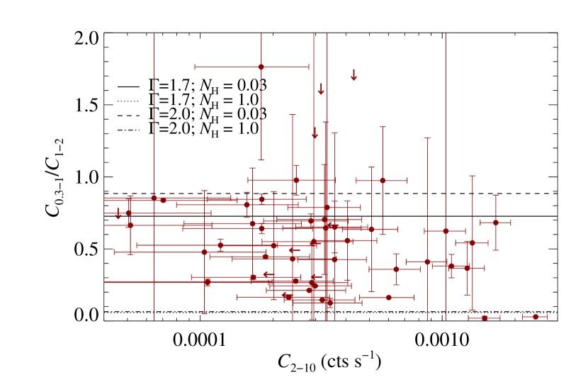
[rgb]0.54,0,0bookmarkcolor colorintensitycolorintensityFig 5: Color-intensity plot of off-nuclear sources.Fig 5: Color-intensity plot of off-nuclear sources. [rgb]0,0,0bookmarkcolor

4. Summary

In this paper we have presented an X-ray survey of 12 galaxies with central black hole mass measurements. The observations were designed to characterize the nuclear source of each galaxy but were sensitive to much more.

1. Each galaxy was observed for 30 ksec with Chandra, and in total we detected 68 point sources in the region of the sky occupied by these galaxies.

2. We detected all 12 nuclear sources with sufficient count rates to model their spectra and determine their X-ray luminosities and Eddington ratios. The sources all were found to be emitting in the 2–10 keV band at $10^{-8}$–$10^{-6}$ of Eddington.

3. When fitting with an absorbed power-law spectral model, we found $\Gamma$, the photon spectral index. Fitting for $\Gamma$ as a function of Eddington fraction, we found a negative correlation, consistent with several earlier reports on low luminosity AGNs. Our best fit was $\Gamma=1.8\pm 0.2-(0.24\pm 0.12)\log(L_{2\textrm{--}10}/10^{-7}L_{\mathrm{Edd}})$ with an rms intrinsic scatter of $0.65\pm 0.20$, which is consistent with predictions from ADAF models, which expect bremsstrahlung emission to become more important at lower accretion rates.

4. Our observations were also sensitive to ULXs in the target galaxies. We found 20 ULX candidates. Based on considerations of the probability distribution of their intrinsic fluxes and the probability of having a background AGN of sufficient brightness to appear as a ULX, we concluded that 6 of these candidates are likely ($>90\%$ chance) to be true ULXs. The most promising ULX candidate is in NGC 2748 and has an isotropic luminosity of $L_{0.3\textrm{--}10}=1.03_{-0.27}^{+0.57}\times 10^{40}\ \mathrm{erg\ s^{-1}}$.

5. We also present a color-intensity plot of the remaining point sources, most of which are likely to be X-ray binaries local to the galaxy.

This work will be followed up with EVLA observations of the nuclear sources. When combining radio and X-ray data, we will be able to provide a complete mass-calibrated fundamental plane that will allow for the estimation of black hole masses using X-ray and radio observations. We will also, with the possible addition of archival sub-millimeter data, broad-band spectral energy distribution modeling.

Figure 6.— X-ray spectra, folded through the instrument response, of the first half of the sample. The spectra are binned for visualization purposes her. The solid line shows the best-fit model. The second half of the sample is in Figure 7. Error bars show 1$\sigma$ uncertainties.

[rgb]0.54,0,0bookmarkcolor spectraspectraFig 6: Spectra of nuclear sources.Fig 6: Spectra of nuclear sources. [rgb]0,0,0bookmarkcolor

Figure 7.— Same as Figure 6 for the second half of the sample. Error bars show 1$\sigma$ uncertainties.

[rgb]0.54,0,0bookmarkcolor spectra2spectra2Fig 7: Spectra of nuclear sources, continued.Fig 7: Spectra of nuclear sources, continued. [rgb]0,0,0bookmarkcolor

Figure 8.— X-ray spectra of strong ULX candidates. Error bars show 1$\sigma$ uncertainties. The solid lines are power-law models in which the $N_{H}$ parameter was allowed to vary above the Galactic value; the dashed lines are models with $N_{H}$ fixed at the Galactic value towards each source.

[rgb]0.54,0,0bookmarkcolor ulxspectraulxspectraFig 8: Spectra of ULX candidates.Fig 8: Spectra of ULX candidates. [rgb]0,0,0bookmarkcolor

Table 5Chandra point source detections

Galaxy	ID	Source name	RA	Dec	Class.	0.3–1 keV		1–2 keV		2–10 keV
(1)	(2)	(3)	(4)	(5)	(6)	(7)		(8)		(9)
NGC1300	1	CXOU J031935.0$-$192509	03:19:35.07	$-$19:25:09.9		$4.5$	$\pm 1.3$	$0.7$	$\pm 0.6$	$<3.2$
…	2	CXOU J031935.1$-$192417	03:19:35.10	$-$19:24:17.4		$0.8$	$\pm 0.6$	$1.5$	$\pm 0.8$	$<3.2$
…	3	CXOU J031935.4$-$192417	03:19:35.49	$-$19:24:17.6		$2.0$	$\pm 0.8$	$2.7$	$\pm 1.0$	$0.5$	$\pm 0.5$
…	4	CXOU J031936.7$-$192500	03:19:36.78	$-$19:25:00.3		$<2.0$		$<2.0$		$<3.8$
…	5	CXOU J031937.8$-$192607	03:19:37.88	$-$19:26:07.8		$0.9$	$\pm 0.6$	$5.6$	$\pm 1.4$	$6.0$	$\pm 1.6$
…	6	CXOU J031937.9$-$192441	03:19:37.95	$-$19:24:41.4	ULX	$4.7$	$\pm 1.3$	$11.0$	$\pm 1.9$	$2.4$	$\pm 1.1$
…	7	CXOU J031938.2$-$192413	03:19:38.21	$-$19:24:13.5		$1.3$	$\pm 0.7$	$2.0$	$\pm 0.8$	$0.5$	$\pm 0.5$
…	8	CXOU J031938.4$-$192318	03:19:38.45	$-$19:23:18.0		$1.6$	$\pm 0.8$	$2.4$	$\pm 1.0$	$<3.7$
…	9	CXOU J031938.5$-$192452	03:19:38.58	$-$19:24:52.4	ULX	$2.5$	$\pm 1.0$	$4.0$	$\pm 1.2$	$1.8$	$\pm 1.0$
…	10	CXOU J031939.3$-$192422	03:19:39.37	$-$19:24:22.8		$2.2$	$\pm 0.9$	$3.2$	$\pm 1.1$	$2.9$	$\pm 1.1$
…	11	CXOU J031939.4$-$192616	03:19:39.47	$-$19:26:16.0		$<2.6$		$1.6$	$\pm 0.8$	$3.2$	$\pm 1.2$
…	12	CXOU J031939.9$-$192550	03:19:39.93	$-$19:25:50.4	ULX	$3.2$	$\pm 1.1$	$5.8$	$\pm 1.4$	$2.9$	$\pm 1.2$
…	13	CXOU J031941.0$-$192440	03:19:41.06	$-$19:24:40.3	Nuc.	$5.5$	$\pm 1.5$	$12.0$	$\pm 2.1$	$27.3$	$\pm 3.1$
…	14	CXOU J031941.3$-$192334	03:19:41.37	$-$19:23:34.2		$3.0$	$\pm 1.0$	$5.7$	$\pm 1.4$	$1.2$	$\pm 0.8$
…	15	CXOU J031942.5$-$192450	03:19:42.50	$-$19:24:50.7		$0.9$	$\pm 0.7$	$3.7$	$\pm 1.2$	$3.0$	$\pm 1.1$
…	16	CXOU J031942.9$-$192511	03:19:42.95	$-$19:25:11.2		$1.2$	$\pm 0.7$	$1.7$	$\pm 0.8$	$3.3$	$\pm 1.3$
…	17	CXOU J031945.9$-$192449	03:19:45.98	$-$19:24:49.3		$<2.4$		$3.1$	$\pm 1.1$	$<4.1$
NGC2748	18	CXOU J091337.4$+$762811	09:13:37.45	$+$76:28:11.4	ULX	$0.6$	$\pm 0.5$	$19.8$	$\pm 2.6$	$24.3$	$\pm 2.9$
…	19	CXOU J091339.6$+$762800	09:13:39.64	$+$76:28:00.5		$<2.6$		$1.9$	$\pm 0.8$	$3.0$	$\pm 1.1$
…	20	CXOU J091340.0$+$762813	09:13:40.01	$+$76:28:13.3		$1.9$	$\pm 0.8$	$3.6$	$\pm 1.1$	$2.0$	$\pm 0.9$
…	21	CXOU J091343.0$+$762831	09:13:43.04	$+$76:28:31.8	Nuc.	$1.9$	$\pm 0.9$	$4.5$	$\pm 1.3$	$1.1$	$\pm 0.8$
…	22	CXOU J091343.8$+$762835	09:13:43.80	$+$76:28:35.9	ULX	$1.5$	$\pm 0.8$	$4.9$	$\pm 1.3$	$1.7$	$\pm 0.8$
…	23	CXOU J091344.4$+$762829	09:13:44.42	$+$76:28:29.3	ULX	$0.6$	$\pm 0.5$	$4.6$	$\pm 1.3$	$3.4$	$\pm 1.1$
…	24	CXOU J091348.5$+$762902	09:13:48.52	$+$76:29:02.2	ULX	$0.3$	$\pm 0.4$	$15.1$	$\pm 2.3$	$15.0$	$\pm 2.3$
…	25	CXOU J091348.9$+$762828	09:13:48.99	$+$76:28:28.5	ULX	$30.3$	$\pm 3.2$	$44.4$	$\pm 3.9$	$16.7$	$\pm 2.4$
NGC2778	26	CXOU J091222.4$+$350135	09:12:22.45	$+$35:01:35.2	ULX	$3.7$	$\pm 1.1$	$4.7$	$\pm 1.3$	$3.3$	$\pm 1.1$
…	27	CXOU J091224.4$+$350139	09:12:24.40	$+$35:01:39.4	Nuc.	$4.8$	$\pm 1.4$	$3.1$	$\pm 1.2$	$1.7$	$\pm 1.0$
NGC3384	28	CXOU J104813.9$+$123839	10:48:13.94	$+$12:38:39.4		$0.6$	$\pm 0.5$	$3.4$	$\pm 1.1$	$2.3$	$\pm 1.0$
…	29	CXOU J104815.1$+$123658	10:48:15.18	$+$12:36:58.7		$6.1$	$\pm 1.5$	$16.6$	$\pm 2.4$	$12.7$	$\pm 2.2$
…	30	CXOU J104816.1$+$123658	10:48:16.15	$+$12:36:58.7	ULX	$1.4$	$\pm 0.7$	$2.8$	$\pm 1.0$	$<2.6$
…	31	CXOU J104816.2$+$123644	10:48:16.27	$+$12:36:44.1		$0.7$	$\pm 0.5$	$2.1$	$\pm 0.9$	$<2.0$
…	32	CXOU J104816.9$+$123745	10:48:16.97	$+$12:37:45.7	Nuc.	$10.7$	$\pm 2.0$	$18.7$	$\pm 2.6$	$9.8$	$\pm 2.0$
…	33	CXOU J104817.4$+$123720	10:48:17.47	$+$12:37:20.8		$1.0$	$\pm 0.6$	$2.0$	$\pm 0.9$	$1.0$	$\pm 0.7$
…	34	CXOU J104819.4$+$123646	10:48:19.41	$+$12:36:46.0	ULX	$1.0$	$\pm 0.6$	$2.4$	$\pm 0.9$	$3.6$	$\pm 1.2$
…	35	CXOU J104820.8$+$123839	10:48:20.81	$+$12:38:39.4	ULX	$3.8$	$\pm 1.2$	$4.5$	$\pm 1.3$	$0.7$	$\pm 0.6$
NGC4291	36	CXOU J122012.1$+$752203	12:20:12.16	$+$75:22:03.1		$1.3$	$\pm 0.8$	$1.5$	$\pm 0.8$	$1.8$	$\pm 0.8$
…	37	CXOU J122016.1$+$752218	12:20:16.12	$+$75:22:18.0	ULX	$2.1$	$\pm 1.3$	$7.7$	$\pm 1.8$	$1.1$	$\pm 0.9$
…	38	CXOU J122016.5$+$752151	12:20:16.50	$+$75:21:51.3		$<3.6$		$2.1$	$\pm 0.9$	$4.3$	$\pm 1.3$
…	39	CXOU J122017.8$+$752214	12:20:17.84	$+$75:22:14.8	Nuc.	$6.6$	$\pm 1.7$	$7.7$	$\pm 1.7$	$6.6$	$\pm 1.5$
…	40	CXOU J122019.8$+$752216	12:20:19.83	$+$75:22:16.2	ULX	$9.3$	$\pm 2.4$	$15.0$	$\pm 2.5$	$10.4$	$\pm 2.0$
…	41	CXOU J122023.6$+$752202	12:20:23.67	$+$75:22:02.5		$1.0$	$\pm 0.9$	$3.4$	$\pm 1.2$	$<3.2$
NGC4459	42	CXOU J122900.0$+$135842	12:29:00.02	$+$13:58:42.0	Nuc.	$18.5$	$\pm 2.6$	$17.2$	$\pm 2.5$	$13.6$	$\pm 2.3$
…	43	CXOU J122900.5$+$135825	12:29:00.56	$+$13:58:25.9	ULX	$1.2$	$\pm 0.7$	$4.3$	$\pm 1.2$	$2.5$	$\pm 1.0$
…	44	CXOU J122900.6$+$135838	12:29:00.62	$+$13:58:38.3		$4.8$	$\pm 1.3$	$12.6$	$\pm 2.1$	$10.9$	$\pm 1.9$
…	45	CXOU J122900.8$+$135843	12:29:00.88	$+$13:58:43.6		$<3.4$		$2.4$	$\pm 1.0$	$<2.4$
NGC4486A	46	CXOU J123057.7$+$121616	12:30:57.77	$+$12:16:16.3		$3.5$	$\pm 1.3$	$5.5$	$\pm 1.6$	$3.3$	$\pm 1.2$
…	47	CXOU J123057.8$+$121614	12:30:57.87	$+$12:16:14.5	Nuc.	$2.4$	$\pm 1.0$	$2.6$	$\pm 1.1$	$3.2$	$\pm 1.1$
NGC4596	48	CXOU J123955.9$+$101033	12:39:55.99	$+$10:10:33.7	Nuc.	$4.4$	$\pm 1.3$	$4.1$	$\pm 1.2$	$2.2$	$\pm 0.9$
…	49	CXOU J123956.0$+$101036	12:39:56.05	$+$10:10:36.0		$4.0$	$\pm 1.2$	$7.3$	$\pm 1.5$	$4.1$	$\pm 1.2$
…	50	CXOU J123956.4$+$101026	12:39:56.43	$+$10:10:26.0		$6.0$	$\pm 1.5$	$9.5$	$\pm 1.8$	$5.1$	$\pm 1.3$
…	51	CXOU J123956.7$+$101101	12:39:56.72	$+$10:11:01.6		$0.5$	$\pm 0.5$	$1.2$	$\pm 0.7$	$1.9$	$\pm 0.9$
…	52	CXOU J123956.8$+$101053	12:39:56.83	$+$10:10:53.1	ULX	$4.7$	$\pm 1.3$	$2.6$	$\pm 1.0$	$1.8$	$\pm 0.9$
…	53	CXOU J123956.9$+$101029	12:39:56.90	$+$10:10:29.8		$3.4$	$\pm 1.1$	$3.5$	$\pm 1.1$	$5.7$	$\pm 1.4$
NGC4742	54	CXOU J125147.6$-$102722	12:51:47.60	$-$10:27:22.6		$4.9$	$\pm 1.3$	$12.1$	$\pm 1.9$	$8.7$	$\pm 1.7$
…	55	CXOU J125147.9$-$102719	12:51:47.92	$-$10:27:19.7	ULX	$0.6$	$\pm 0.5$	$4.3$	$\pm 1.2$	$3.2$	$\pm 1.1$
…	56	CXOU J125148.0$-$102717	12:51:48.07	$-$10:27:17.2	Nuc.	$14.9$	$\pm 2.2$	$18.0$	$\pm 2.4$	$12.9$	$\pm 2.1$
…	57	CXOU J125148.2$-$102710	12:51:48.27	$-$10:27:10.8	ULX	$2.4$	$\pm 0.9$	$3.6$	$\pm 1.1$	$1.6$	$\pm 0.9$
…	58	CXOU J125149.3$-$102727	12:51:49.34	$-$10:27:27.4		$8.4$	$\pm 1.6$	$15.5$	$\pm 2.2$	$13.3$	$\pm 2.1$
NGC5077	59	CXOU J131931.6$-$123925	13:19:31.66	$-$12:39:25.1	Nuc.	$12.1$	$\pm 2.5$	$16.4$	$\pm 2.6$	$13.6$	$\pm 2.3$
…	60	CXOU J131931.9$-$123938	13:19:31.93	$-$12:39:38.3		$1.7$	$\pm 0.9$	$2.1$	$\pm 0.9$	$1.6$	$\pm 0.9$
NGC5576	61	CXOU J142102.7$+$031611	14:21:02.76	$+$03:16:11.6	ULX	$0.8$	$\pm 0.6$	$3.2$	$\pm 1.1$	$2.9$	$\pm 1.1$
…	62	CXOU J142102.9$+$031621	14:21:02.97	$+$03:16:21.6		$1.0$	$\pm 0.7$	$3.5$	$\pm 1.2$	$1.1$	$\pm 0.8$
…	63	CXOU J142103.7$+$031614	14:21:03.71	$+$03:16:14.9	Nuc.	$5.1$	$\pm 1.4$	$8.4$	$\pm 1.8$	$2.7$	$\pm 1.1$
…	64	CXOU J142105.1$+$031615	14:21:05.18	$+$03:16:15.9	ULX	$2.6$	$\pm 1.0$	$2.6$	$\pm 1.0$	$2.5$	$\pm 1.0$
NGC7457	65	CXOU J230058.0$+$300850	23:00:58.07	$+$30:08:50.5		$0.7$	$\pm 0.5$	$3.1$	$\pm 1.1$	$2.8$	$\pm 1.1$
…	66	CXOU J230059.1$+$300907	23:00:59.16	$+$30:09:07.4		$0.6$	$\pm 0.5$	$1.7$	$\pm 0.8$	$6.5$	$\pm 1.6$
…	67	CXOU J230059.9$+$300841	23:00:59.95	$+$30:08:41.8	Nuc.	$3.2$	$\pm 1.1$	$7.5$	$\pm 1.6$	$4.3$	$\pm 1.4$
…	68	CXOU J230101.1$+$300900	23:01:01.19	$+$30:09:00.7		$3.4$	$\pm 1.1$	$5.2$	$\pm 1.4$	$3.6$	$\pm 1.2$

Note. — List of X-ray point sources detected in the field of each galaxy. Columns list: (1) the name of the galaxy in which the sources appear to lie; (2) a running identification number used in this paper; (3) IAU approved source name for each source; (4) and (5) J2000 coordinates for each source; (6) classification of each source, where Nuc. indicates the source is nuclear source and presumed to be the SMBH for its galaxy, and ULX indicates that it is a ULX candidate; (7), (8), and (9) are the count rates for each source in the given bands in units of $10^{-4}\ \mathrm{cts\ s^{-1}}$. If a source is consistent with no flux in a given band, then we list the $3\sigma$ upper limit, otherwise we list the $1\sigma$ uncertainty.

[rgb]0,0,0.54bookmarkcolor table.0table.0Table 5: X-ray point sourcesTable 5: X-ray point sources [rgb]0,0,0bookmarkcolor

References

- Arnaud (1996) Arnaud, K. A. 1996, in Astronomical Society of the Pacific Conference Series 101, Astronomical Data Analysis Software and Systems V, ed. G. H. Jacoby & J. Barnes, 17
- Atkinson et al. (2005) Atkinson, J. W., Collett, J. L., Marconi, A., et al. 2005, MNRAS, 359, 504
- Bajaja et al. (2005) Bajaja, E., Arnal, E. M., Larrarte, J. J., Morras, R., Pöppel, W. G. L., & Kalberla, P. M. W. 2005, A&A, 440, 767
- Barth et al. (2001) Barth, A. J., Sarzi, M., Rix, H.-W., Ho, L. C., Filippenko, A. V., & Sargent, W. L. W. 2001, ApJ, 555, 685
- Begelman (2002) Begelman, M. C. 2002, ApJ, 568, L97
- Begelman (2006) ———. 2006, ApJ, 636, 995
- Bell (2003) Bell, E. F. 2003, ApJ, 586, 794
- Bentz et al. (2006) Bentz, M. C., Denney, K. D., Cackett, E. M., et al. 2006, ApJ, 651, 775
- Blandford & Payne (1982) Blandford, R. D., & Payne, D. G. 1982, MNRAS, 199, 883
- Blandford & Znajek (1977) Blandford, R. D., & Znajek, R. L. 1977, MNRAS, 179, 433
- Cash (1979) Cash, W. 1979, ApJ, 228, 939
- Constantin et al. (2009) Constantin, A., Green, P., Aldcroft, T., Kim, D.-W., Haggard, D., Barkhouse, W., & Anderson, S. F. 2009, ApJ, 705, 1336
- Corbel et al. (2006) Corbel, S., Tomsick, J. A., & Kaaret, P. 2006, ApJ, 636, 971
- de Francesco et al. (2008) de Francesco, G., Capetti, A., & Marconi, A. 2008, A&A, 479, 355
- de Gasperin et al. (2011) de Gasperin, F., Merloni, A., Sell, P., Best, P., Heinz, S., & Kauffmann, G. 2011, MNRAS, 835
- Di Matteo et al. (2005) Di Matteo, T., Springel, V., & Hernquist, L. 2005, Nature, 433, 604
- Esin et al. (1997) Esin, A. A., McClintock, J. E., & Narayan, R. 1997, ApJ, 489, 865
- Faber et al. (1989) Faber, S. M., Wegner, G., Burstein, D., Davies, R. L., Dressler, A., Lynden-Bell, D., & Terlevich, R. J. 1989, ApJS, 69, 763
- Fabian (1999) Fabian, A. C. 1999, MNRAS, 308, L39
- Falcke et al. (2004) Falcke, H., Körding, E., & Markoff, S. 2004, A&A, 414, 895
- Farrell et al. (2009) Farrell, S. A., Webb, N. A., Barret, D., Godet, O., & Rodrigues, J. M. 2009, Nature, 460, 73
- Gebhardt et al. (2003) Gebhardt, K., Richstone, D., Tremaine, S., et al. 2003, ApJ, 583, 92
- Giacconi et al. (2001) Giacconi, R., Rosati, P., Tozzi, P., et al. 2001, ApJ, 551, 624
- Graham et al. (2011) Graham, A. W., Onken, C. A., Athanassoula, E., & Combes, F. 2011, MNRAS, 412, 2211
- Grimm et al. (2003) Grimm, H.-J., Gilfanov, M., & Sunyaev, R. 2003, MNRAS, 339, 793
- Gu & Cao (2009) Gu, M., & Cao, X. 2009, MNRAS, 399, 349
- Gültekin et al. (2009a) Gültekin, K., Cackett, E. M., Miller, J. M., Di Matteo, T., Markoff, S., & Richstone, D. O. 2009a, ApJ, 706, 404
- Gültekin et al. (2004) Gültekin, K., Miller, M. C., & Hamilton, D. P. 2004, ApJ, 616, 221
- Gültekin et al. (2006) ———. 2006, ApJ, 640, 156
- Gültekin et al. (2009b) Gültekin, K., Richstone, D. O., Gebhardt, K., et al. 2009b, ApJ, 695, 1577
- Gültekin et al. (2009c) ———. 2009c, ApJ, 698, 198
- Ho (2008) Ho, L. C. 2008, ARA&A, 46, 475
- Ho et al. (1997) Ho, L. C., Filippenko, A. V., Sargent, W. L. W., & Peng, C. Y. 1997, ApJS, 112, 391
- Irwin et al. (2003) Irwin, J. A., Athey, A. E., & Bregman, J. N. 2003, ApJ, 587, 356
- Kaaret et al. (2004) Kaaret, P., Ward, M. J., & Zezas, A. 2004, MNRAS, 351, L83
- Kennicutt (1998) Kennicutt, R. C., Jr. 1998, ARA&A, 36, 189
- Kim & Fabbiano (2004) Kim, D.-W., & Fabbiano, G. 2004, ApJ, 611, 846
- King et al. (2001) King, A. R., Davies, M. B., Ward, M. J., Fabbiano, G., & Elvis, M. 2001, ApJ, 552, L109
- Knapp et al. (1989) Knapp, G. R., Guhathakurta, P., Kim, D.-W., & Jura, M. A. 1989, ApJS, 70, 329
- Körding et al. (2006) Körding, E., Falcke, H., & Corbel, S. 2006, A&A, 456, 439
- Kuo et al. (2011) Kuo, C. Y., Braatz, J. A., Condon, J. J., et al. 2011, ApJ, 727, 20
- Li et al. (2008) Li, Z.-Y., Wu, X.-B., & Wang, R. 2008, ApJ, 688, 826
- Lynden-Bell (1978) Lynden-Bell, D. 1978, Phys. Scr, 17, 185
- Mei et al. (2007) Mei, S., Blakeslee, J. P., Côté, P., et al. 2007, ApJ, 655, 144
- Merloni et al. (2003) Merloni, A., Heinz, S., & Di Matteo, T. 2003, MNRAS, 345, 1057
- Merloni et al. (2006) Merloni, A., Körding, E., Heinz, S., Markoff, S., Di Matteo, T., & Falcke, H. 2006, New Astronomy, 11, 567
- Miller & Hamilton (2002) Miller, M. C., & Hamilton, D. P. 2002, MNRAS, 330, 232
- Mushotzky (1984) Mushotzky, R. F. 1984, Advances in Space Research, 3, 157
- Nowak et al. (2007) Nowak, N., Saglia, R. P., Thomas, J., Bender, R., Pannella, M., Gebhardt, K., & Davies, R. I. 2007, MNRAS, 379, 909
- Onken et al. (2004) Onken, C. A., Ferrarese, L., Merritt, D., Peterson, B. M., Pogge, R. W., Vestergaard, M., & Wandel, A. 2004, ApJ, 615, 645
- Pakull & Mirioni (2001) Pakull, M. W., & Mirioni, L. 2001, in Astronomische Gesellschaft Meeting Abstracts, 112
- Plotkin et al. (2011) Plotkin, R. M., Markoff, S., Kelly, B. C., Koerding, E., & Anderson, S. F. 2011, preprint (1105.3211)
- Portegies Zwart et al. (2004) Portegies Zwart, S. F., Baumgardt, H., Hut, P., Makino, J., & McMillan, S. L. W. 2004, Nature, 428, 724
- Protassov et al. (2002) Protassov, R., van Dyk, D. A., Connors, A., Kashyap, V. L., & Siemiginowska, A. 2002, ApJ, 571, 545
- Rees (1984) Rees, M. J. 1984, ARA&A, 22, 471
- Richstone et al. (1998) Richstone, D., Ajhar, E. A., Bender, R., et al. 1998, Nature, 395, A14
- Rosa-González et al. (2002) Rosa-González, D., Terlevich, E., & Terlevich, R. 2002, MNRAS, 332, 283
- Sarzi et al. (2001) Sarzi, M., Rix, H.-W., Shields, J. C., Rudnick, G., Ho, L. C., McIntosh, D. H., Filippenko, A. V., & Sargent, W. L. W. 2001, ApJ, 550, 65
- Schawinski et al. (2007) Schawinski, K., Thomas, D., Sarzi, M., Maraston, C., Kaviraj, S., Joo, S.-J., Yi, S. K., & Silk, J. 2007, MNRAS, 382, 1415
- Shemmer et al. (2008) Shemmer, O., Brandt, W. N., Netzer, H., Maiolino, R., & Kaspi, S. 2008, ApJ, 682, 81
- Silk & Rees (1998) Silk, J., & Rees, M. J. 1998, A&A, 331, L1
- Skrutskie et al. (2006) Skrutskie, M. F., Cutri, R. M., Stiening, R., et al. 2006, AJ, 131, 1163
- Smith et al. (2001) Smith, R. K., Brickhouse, N. S., Liedahl, D. A., & Raymond, J. C. 2001, ApJ, 556, L91
- Temi et al. (2009) Temi, P., Brighenti, F., & Mathews, W. G. 2009, ApJ, 695, 1
- Tonry et al. (2001) Tonry, J. L., Dressler, A., Blakeslee, J. P., Ajhar, E. A., Fletcher, A. B., Luppino, G. A., Metzger, M. R., & Moore, C. B. 2001, ApJ, 546, 681
- Tully (1988) Tully, R. B. 1988, Nearby galaxies catalog, ed. Tully, R. B.
- Vasudevan & Fabian (2007) Vasudevan, R. V., & Fabian, A. C. 2007, MNRAS, 381, 1235
- Véron-Cetty & Véron (2006) Véron-Cetty, M.-P., & Véron, P. 2006, A&A, 455, 773
- Véron-Cetty & Véron (2010) ———. 2010, A&A, 518, A10+
- Walton et al. (2011) Walton, D. J., Roberts, T. P., Mateos, S., & Heard, V. 2011, MNRAS, 1147
- Wang et al. (2006) Wang, R., Wu, X.-B., & Kong, M.-Z. 2006, ApJ, 645, 890
- Watson et al. (2009) Watson, M. G., Schröder, A. C., Fyfe, D., et al. 2009, A&A, 493, 339
- Winter et al. (2009) Winter, L. M., Mushotzky, R. F., Reynolds, C. S., & Tueller, J. 2009, ApJ, 690, 1322
- Younes et al. (2011) Younes, G., Porquet, D., Sabra, B., & Reeves, J. N. 2011, A&A, 530, A149+
- Yuan et al. (2009) Yuan, F., Yu, Z., & Ho, L. C. 2009, ApJ, 703, 1034
[rgb]0.54,0,0bookmarkcolor \EdefEscapeHexspectraspectra\EdefEscapeHexFig 6: Spectra of nuclear sources.Fig 6: Spectra of nuclear sources. \HyColor@BookmarkColor[rgb]0,0,0bookmarkcolor
[rgb]0.54,0,0bookmarkcolor \EdefEscapeHexspectra2spectra2\EdefEscapeHexFig 7: Spectra of nuclear sources, continued.Fig 7: Spectra of nuclear sources, continued. \HyColor@BookmarkColor[rgb]0,0,0bookmarkcolor
[rgb]0.54,0,0bookmarkcolor \EdefEscapeHexulxspectraulxspectra\EdefEscapeHexFig 8: Spectra of ULX candidates.Fig 8: Spectra of ULX candidates. \HyColor@BookmarkColor[rgb]0,0,0bookmarkcolor