Magnetic anisotropies of quantum dots

Abstract

Magnetic anisotropies in quantum dots (QDs) doped with magnetic ions are discussed in terms of two frameworks: anisotropic $g$-factors and magnetocrystalline anisotropy energy. It is shown that even a simple model of zinc-blende p-doped QDs displays a rich diagram of magnetic anisotropies in the QD parameter space. Tuning the confinement allows to control magnetic easy axes in QDs in ways not available for the better-studied bulk.

I Introduction

Once the origin of magnetic ordering in a specific material is understood, it is often important to determine its magnetic anisotropy (MA) and hard and easy magnetic axes in particular. A shift of focus towards MA has already occurred for the studies of bulk dilute magnetic semiconductors (DMS),Welp2003:PRL ; Liu2003:PRB but not yet fully for magnetic quantum dots (QDs) where it could play certain role, for example, in context of transport phenomena,Fernandez-Rossier2011:bookCh the formation of robust magnetic polarons,Yakovlev2010:bookCh ; Beaulac2009:Sci ; Sellers2010:PRB ; Henneberger2010:bookCh control of magnetic ordering,Abolfath2008:PRL ; Govorov-twice ; Oszwaldowski2011:PRL ; Bussian2009:NMat ; Ochsenbein2009:nnano nonvolatile memory,Enaya2008:JAP and quantum bits.LeGall2010:PRB

In epilayers of (Ga,Mn)As, a prototypical DMS, the magnetocrystalline anisotropy energy (MAE) has been found to be a significant and often dominant source of MAZemen2009:PRB ; Dreher2010:PRB ; Linnik2011:arxiv caused by a strong spin-orbit (SO) coupling. It turns out that the easy axis direction depends on hole concentration, magnetic doping level as well as on other parameters. For example, when (Ga,Mn)As was used as a spin injector, the effects of strain (by altering the choice of a substrate) were responsible for changing the in-plane to out-plane easy axis.Zutic2004:RMP While the strong SO couplingFabian2007:APS is also present in p-type QD of zinc-blende materials doped with Mn, its effect on magnetic anisotropies will be significantly modified by the confinement. The energy levels in such ‘nanomagnets,’Bader2006:RMP ; Fernandez-Rossier2007:PRL ; Cheng2009:PRB ; Kyrychenko2004:PRB where the Mn-Mn interaction is mediated by carriers, depend on the magnetization direction $\mathbf{e}_{M}=(n_{x},n_{y},n_{z})$. It is often assumed that the interaction of magnetic moments with holes in quantum wells (QWs) or, equivalently in flat QDs, is effectively Ising-like.LeGall2010:PRB ; Lee2000:PRB Here we quantify this assumption and explore MA using two frameworks: (i) an effective two-level Hamiltonian with a carrier $g$–tensor,Merkulov1995:PRB which is widely employed also in theory of electron spin resonance, and (ii) MAE, which is commonly used to study bulk magnets.

While previous studies focused on specific nonmagnetic QDsPryor2006:PRL and properties sensitive to system details (such as precise position of magnetic ionsCheng2009:PRB ; Bhattacharjee2007:PRB ), we explore more generic magnetic QD models, which can also serve as a starting point for more elaborate work. We consider a Hamiltonian comprising non-magnetic and magnetic parts,

$$\hat{H}=\hat{H}_{QD}+\hat{H}_{ex}.$$ (1)

The former encodes both QD confinement and SO interaction, which is prerequisite for magnetic anisotropies, the latter expresses the kinetic-exchange coupling between holes and localized magnetic moments. For transparency, we disregard the magnetostatic shape anisotropyshapeAniso2 and assume that the QD contains a fixed number of carriers. We mostly focus on the case of a single hole; realistically, such system can be a II-VI colloidalBeaulac2009:Sci or epitaxialSellers2010:PRB QD with a photoinduced carrier. Magnetic moments of the Mn atoms are taken to be perfectly ordered (collinear) and are treated at a mean-field level. The magnetic easy axis is then the direction $\mathbf{e}_{M}$ for which the zero-temperature free energy $F(\mathbf{e}_{M})$ is minimized. In this article, we take two different points of view on $F(\mathbf{e}_{M})$. On one hand, we discuss the lowest terms of $F(\mathbf{e}_{M})$ expanded in powers of the direction cosines of magnetization ($n_{x}^{2}+n_{y}^{2}+n_{z}^{2}=1$), inspired by the standard ‘bulk MAE phenomenology’ and pay special attention to the case of perfectly cubic QDs, $F(\mathbf{e}_{M})=F_{0}(\mathbf{e}_{M})$. The anisotropies in $F_{0}$ stem purely from the crystalline zinc-blende lattice. On the other hand, $F(\mathbf{e}_{M})$ acquires additional terms in systems with less symmetric confinement. We therefore discuss the anisotropic $g$-factors as a useful framework to handle such systems, e.g. cuboid QDs (orthogonal parallelepiped; extremal cases are a cube and an infinitely thin slab, i.e., a QW) and show how the expansion

$$F(\mathbf{e}_{M})=F_{0}(\mathbf{e}_{M})+AF_{1}(\mathbf{e}_{M})+A^{2}F_{2}(\mathbf{e}_{M})+\ldots$$ (2)

can be constructed using powers of $A$ which reflects the anisotropy in $g$-factors. We begin by discussing this latter topic in Section II (quantity $A$ is defined by Eq. (8) at the end of Sec. IIA), then proceed to the phenomenologic (symmetry-based) expansions of $F_{0}$ in Section III and conclude that Section with calculations of $F_{1}$ in situations that are beyond the applicability of the $g$-factor framework.

II Effective two-level Hamiltonian

Since $\hat{H}_{QD}$ is invariant upon time reversal, its spectrum consists of Kramers doublets.KramersDbl To study the ground-state energy in the presence of magnetic moments, we examine how these doublets are split by $\hat{H}_{ex}(\mathbf{e}_{M})$ where $\mathbf{e}_{M}$ is treated as an external parameter (related to classical magnetization; single-Mn doped QDs where the Mn magnetic moment behaves quantum-mechanicallysingleMn require different treatment) and represent them by an effective two-level Hamiltonian of Eq. (6). We consider two example systems: a simple four-level one where completely analytical treatment is possible, and a more realistic envelope-function based model of a cuboid QD.

II.1 Four level model

Related to the Kohn-Luttinger Hamiltonian of a QW,Merkulov2010:bookCh ; Kyrychenko2004:PRB the arguably simplest non-trivial model describing anisotropy of a flat QD is

$$\hat{H}_{1}=a\hat{J}_{z}^{2}+\frac{1}{3}h\mathbf{e}_{M}\cdot\hat{\mathbf{J}}$$ (3)

representing hole levels in a zinc-blende structure whose confinement anisotropy and exchange splitting are parametrized by $a$ and $h$, respectively (the term $a\hat{J}_{z}^{2}$ implies that the strongest confinement is along the $z$-direction and this term also encodes information about the SO coupling). $\hat{J}_{x,y,z}$ are $4\times 4$ spin-$\frac{3}{2}$ matrices. In terms of Eq. (1), we now choose $\hat{H}=\hat{H}_{1}$ and the first (second) term in Eq. (3) plays the role of $\hat{H}_{QD}$ ($\hat{H}_{ex}$). Anisotropic behavior of eigenvalues of $\hat{H}_{1}$, to linear order in $h/a$, is illustrated in Fig. 1(a). It can be extracted from the exact eigenvalues,

$$E_{hh}^{\pm}(h) = \frac{5}{4}a\pm\frac{1}{6}h+\sqrt{a^{2}+\frac{1}{9}h^{2}\mp\frac{1}{3}ah}$$ (4)

$$E_{lh}^{\pm}(h) = \frac{5}{4}a\pm\frac{1}{6}h-\sqrt{a^{2}+\frac{1}{9}h^{2}\mp\frac{1}{3}ah}$$ (5)

in the case $n_{x}=1$ (or $n_{y}=1$), shown in Fig. 1(b), which clearly differ from the case $n_{z}=1$ where the eigenvalues are strictly linear functions of $h$ ($E_{hh}^{\pm}=9a/4\pm h/2$ and $E_{lh}^{\pm}=a/4\pm h/6$); subscripts refer to the $E_{hh}^{\pm}(0)=9a/4$ (‘heavy-hole’, HH) and $E_{lh}^{\pm}(0)=a/4$ (‘light-hole’, LH) doublets, respectively. In the limit of weak exchange, $h/a\ll 1$, splitting of each of the Kramers doublets is symmetric and it can be characterized by three parameters $|\partial E/\partial(hn_{p})|$, $p=x,y,z$, for $h\to 0$ as depicted in Fig. 1(a). These parameters can be plausibly called, by analogy with the Zeeman effect, the anisotropic $g$-factors $g_{p}$. From Eqs. (4),(5), we straightforwardly obtain $(g_{x},g_{y},g_{z})=(0,0,1/2)$ and $(1/3,1/3,1/6)$ for the HH and LH doublet of the Hamiltonian $\hat{H}_{1}$, respectively. This result is known from the context of QWs.Merkulov2010:bookCh ; Petukhov1996:PRB We emphasize that these $g$-factors of the model specified by Eq. (3) are independent of the parameters $a,h$ (except for the requirement $h\ll a$ which represents the $h\to 0$ limit).

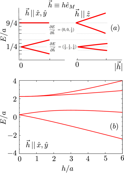
Figure 1: (Color online) Splitting of levels $E(h)$ in a flat QD described by Eq. (3). (a) For the particular Kramers doublet, $E(h)$ depends on $\mathbf{e}_{M}$ and the $g$-factors (by convention non-negative) are $\partial E/\partial\vec{h}=(g_{x},g_{y},g_{z})$. (b) Beyond the linear regime in $h/a$, $\partial E/\partial(hn_{x})$ will be different for the upper and lower level of the split doublet, it will depend on $h$ and may even change sign, indicating that the $\hat{H}_{\rm eff}$ of Eq. (6) based on parameters $g_{x,y,z}$ fails.

If we focus on one particular Kramers doublet, it is straigtforward to show that $\hat{H}_{1}$ projects to

$$\hat{H}_{\rm eff}=h\left[n_{x}g_{x}\hat{\tau}_{x}+n_{y}g_{y}\hat{\tau}_{y}+n_{z}g_{z}\hat{\tau}_{z}\right]$$ (6)

for a suitably chosen basis $|K_{1}\rangle$, $|K_{2}\rangle$ of the doublet. Here $\hat{\tau}_{i}$ are Pauli matrices and we have mapped two eigenstates of the original Hamiltonian $\hat{H}_{QD}$ on a pseudospin $|\vec{\tau}|=1/2$ doublet $|+\rangle$, $|-\rangle$, where $\hat{\tau}_{z}|\pm\rangle=\pm|\pm\rangle$. For $\hat{H}=\hat{H}_{1}$, the eigenstates are only four-dimensional (spanned by the $|J_{z}=3/2\rangle$, $|J_{z}=-1/2\rangle$,$|J_{z}=1/2\rangle$,$|J_{z}=-3/2\rangle$ basis). We present another example of $\hat{H}$ in Sec. IIB where advantage of the projection becomes more apparent. The choice of basis $|+\rangle$, $|-\rangle$ is crucial to obtain $\hat{H}_{\rm eff}$ in the simple form (6); considering the HH doublet: $|+\rangle=|J_{z}=3/2\rangle$, $|-\rangle=|J_{z}=-3/2\rangle$ leads to Eq. (6) while for other basis choices the mapping $\hat{H}_{ex}=(h/3)\mathbf{e}_{M}\cdot\hat{\mathbf{J}}\ \mapsto\ \hat{H}_{\rm eff}=h\mathbf{e}_{M}\cdot g\cdot\hat{\mathbf{\tau}}$ may leadMerkulov2010:bookCh to non-symmetric tensor $g=g_{ij}$, $i,j\in\{x,y,z\}$. In general, if the mapping is to produce $g_{ij}=\mbox{diag }(g_{x},g_{y},g_{z})$ the ‘suitable choice of the basis $|K_{1}\rangle$, $|K_{2}\rangle$’ where $|K_{1}\rangle\mapsto|+\rangle$ is such that $\langle K_{1}|\hat{J}_{x,y}|K_{1}\rangle=0$, $\langle K_{1}|\hat{J}_{z}|K_{1}\rangle\geq 0$ (and $|K_{2}\rangle$ is the time-reversed image of $|K_{1}\rangle$ which is mapped to $|-\rangle$).

Let us now consider a general system described by Eq. (1). Assuming that the downfolding of $\hat{H}$ into $\hat{H}_{\rm eff}$ is possible for given $|K_{1}\rangle$, $|K_{2}\rangle$ (this assumption is discussed in Appendix A), the anisotropic $g$-factors can readily be determined as $\partial E/\partial h$ for the particular Kramers doublet level $E$. This is equivalent to perturbatively evaluating the effect of $\hat{H}_{ex}$ on two degenerate levels to the first order of $h$ as follows: (i) specify the Kramers doublet of interest, and find any basis $|K_{1}\rangle$, $|K_{2}\rangle$ of this doublet, (ii) extract the operators $\hat{t}_{x,y,z}$ from $\hat{H}_{ex}$ by taking $\hat{t}_{p}=\partial\hat{H}_{ex}/\partial(n_{p}h)$ (for example, $\hat{t}_{x}=\hat{J_{x}}/3$ for $\hat{H}_{\rm eff}$ appearing in $\hat{H}_{1}$), (iii) evaluate their matrices

$$\tilde{t}_{x,y,z}=\left(\begin{array}[]{cc}\langle K_{1}|\hat{t}_{x,y,z}|K_{1}\rangle&\langle K_{1}|\hat{t}_{x,y,z}|K_{2}\rangle\\ \langle K_{2}|\hat{t}_{x,y,z}|K_{1}\rangle&\langle K_{2}|\hat{t}_{x,y,z}|K_{2}\rangle\end{array}\right)$$ (7)

in the two-dimensional space spanned by $|K_{1}\rangle$, $|K_{2}\rangle$, and (iv) the non-negative eigenvalue of $\tilde{t}_{p}$ equals $g_{p}$ ($p=x,y,z$). We emphasize that while $g_{p}$ depends on system parameters in $\hat{H}_{QD}$ and $\hat{H}_{ex}$, it also depends on which Kramers doublet we choose. Higher doublets become relevant for QDs containing higher (odd) number of holes, for example.

The effective Hamiltonian in Eq. (6) can be used for various purposes, e.g., for studies of fluctuations of magnetization in magnetic QDsDorozhkin2003:PRB , spin-selective tunneling through non-magnetic QDsKatsaros2011:PRL or excitons in single-Mn doped QDs.LeGall2011:PRL If the magnetic easy axis is of interest, the $g$-factors immediately provide the answer: $F(\mathbf{e}_{M})$ based on Eq. (6) is minimized for $\mathbf{e}_{M}$ in the direction of the largest $g_{p}$ (e.g. for the HH doublet in Fig. 1(a), it is $n_{z}=1$ because $g_{z}>g_{x},g_{y}$). If the full form of $F(\mathbf{e}_{M})$ is needed (e.g, for ferromagnetic resonanceLiu2003:PRB ), it can be straightforwardly obtained by diagonalizing the $2\times 2$ matrix of $\hat{H}_{\rm eff}$. Assuming $g_{x}=g_{y}$, the (modulus of the) eigenvalue can be expanded in terms of parameters $A$ and $k$ as derived in Appendix B. It is meaningful to call

$$A=(g_{z}^{2}-g_{x}^{2})/(g_{z}^{2}+g_{x}^{2})$$ (8)

the asymmetry parameter since it vanishes in a perfectly cubic QD ($g_{x}=g_{y}=g_{z}$) and it is with respect to this parameter that we can identify

$$AF_{1}(\mathbf{e}_{M}) = -Akn_{z}^{2}$$ (9)

$$A^{2}F_{2}(\mathbf{e}_{M}) = +\frac{1}{8}A^{2}k(2n_{z}^{2}-1)^{2}$$ (10)

in Eq. (2) to linear order of $k\propto h$.

II.2 A cuboid quantum dot model

With this general scheme at hand, we take one step in the hierarchy of models towards a more realistic description of magnetic QDs. We consider a zinc-blende structure p-doped semiconductor shaped into a cuboid of size $L_{x}\times L_{y}\times L_{z}$ such as can be described by four-band Kohn-Luttinger Hamiltonian.Kyrychenko2004:PRB Also in this system, $\hat{H}=\hat{H}_{2}$ is a sum of $\hat{H}_{ex}$ and $\hat{H}_{QD}$ but this time, $\hat{H}_{QD}$ comprises of blocks $\langle m_{x}m_{y}m_{z}|\hat{H}_{KL}|m_{x}^{\prime}m_{y}^{\prime}m_{z}^{\prime}\rangle$ with

$$\hat{H}_{KL} = \frac{\hbar^{2}}{2m_{0}}\{\textstyle(\gamma_{1}+\frac{5}{2}\gamma_{2})p^{2}-2\gamma_{2}[\hat{J}_{x}^{2}\hat{p}_{x}^{2}+\hat{J}_{y}^{2}\hat{p}_{y}^{2}+\hat{J}_{z}^{2}\hat{p}_{z}^{2}]$$ (11)

$$-2\gamma_{3}[(\hat{J}_{x}\hat{J}_{y}+\hat{J}_{y}\hat{J}_{x})\hat{p}_{x}\hat{p}_{y}+\mbox{c.p.}]$$

Here, $|m_{x}m_{y}m_{z}\rangle$ denotes the basis of envelope functions, $\gamma_{1,2,3}$ the Luttinger parameters, $m_{0}$ the electron vacuum mass, $\hat{p}_{x,y,z}$ the momentum operators and c.p. denotes the cyclic permutation (see Appendix C for details). The envelope function is conveniently developed into harmonic functions with $m_{p}-1$ nodes in the $p=x,y,z$ direction:

$$\langle\vec{r}|m_{x}m_{y}m_{z}\rangle=N\sin\frac{m_{x}\pi x}{\lambda_{x}L}\sin\frac{m_{y}\pi y}{\lambda_{y}L}\sin\frac{m_{z}\pi z}{L}.$$ (12)

We have introduced the dimensionless aspect ratios $\lambda_{x,y}=L_{x,y}/L$ and the normalization factor $N$. Our system can be viewed as an infinitely deep potential well with $V(x,y,z)=0$ for $0<x<L_{x}$, $0<y<L_{y}$ and $0<z<L_{z}\equiv L$ and infinite otherwise.

For fixed material parameters (Luttinger parameters in ratios $\gamma_{2}/\gamma_{1}$, $\gamma_{3}/\gamma_{2}$) and QD shape ($\lambda_{x},\lambda_{y}$), all matrix elements of all blocks $\langle m_{x}m_{y}m_{z}|\hat{H}_{KL}|m_{x}^{\prime}m_{y}^{\prime}m_{z}^{\prime}\rangle$ scale as $1/L^{2}$. The spectrum, consisting of Kramers doublets which occasionally combine into larger multiplets, is specified by a sequence of dimensionless numbers $E/{\cal E}_{0}$ where

$${\cal E}_{0}=\hbar^{2}\pi^{2}\gamma_{1}/(2m_{0}L^{2}).$$ (13)

For a cubic QD [$\lambda_{x}=\lambda_{y}=1$; see Fig. 2(a)] the s-like state shown in the inset of Fig. 2(a) forms a quadruplet, and depending on the value of $\gamma_{2}/\gamma_{1}$ (and to somehow lesser extent also of $\gamma_{3}/\gamma_{2}$) this state competes with the next doublet for having the lowest energy. The critical value (see Appendix C)

$$c_{R}=(2+128/9\pi^{2})^{-1}\approx 0.29$$ (14)

can be taken to distinguish materials with small ($\gamma_{2}/\gamma_{1}<c_{R}$, ground state quadruplet) and large ($\gamma_{2}/\gamma_{1}>c_{R}$, ground state doublet) splitting between light and heavy holes in the bulk; these can be ZnSe and CdTe, respectively, their values of $\bar{\gamma}_{2}/\gamma_{1}$ based on approximating $\gamma_{2}$ and $\gamma_{3}$ by their average $\bar{\gamma}_{2}=(\gamma_{2}+\gamma_{3})/2$ are indicated in Fig. 2(a). By numerical diagonalization we have determined the lowest 7 Kramers doublets in slightly deformed QDs ($\lambda_{x}=\lambda_{y}\equiv\lambda=1.01$) in these materials ($\gamma_{1/2/3}=4.8/0.67/1.53$ for ZnSe and $4.1/1.1/1.6$ for CdTe)matParam and executed the procedure (i)-(iv) above to obtain the $g$-factors which are listed in the table on the right of Fig. 2 ($g_{x}=g_{y}$ due to $\lambda_{x}=\lambda_{y}$). To avoid confusion, we remark that in (i), $|K_{1}\rangle$, $|K_{2}\rangle$ are vectors of dimension 864 in the basis $|m_{x}m_{y}m_{z}\rangle\otimes|J_{z}\rangle$ (see the discussion of cut-off in Appendix C) and in (ii), $\hat{t}_{x}=(1/3)\hat{J}_{x}\otimes 1\!\!1_{xyz}$, where $1\!\!1_{xyz}$ is the identity operator in the space of the envelope functions given by Eq. (12). Evaluation and diagonalization of the $2\times 2$ matrices in Eq. (7) requested in (iii,iv) is performed numerically. The possibility to map the action of $\hat{H}_{ex}=(h/3)\mathbf{e}_{M}\cdot\hat{\mathbf{J}}\otimes 1\!\!1_{xyz}$ on the Kramers doublets $|K_{1}\rangle$, $|K_{2}\rangle$ implied by $\hat{H}_{QD}$ of a cuboid p-doped QD is discussed in Appendix A.

The slight deformation of the QD makes the quadruplet split into two doublets (with energies $71.7$ and $71.9\ \mathrm{meV}$ for ZnSe) whose $g$-factors approach $(0,0,1/2)$ and $(1/3,1/3,1/6)$. Similar situation occurs for the doublet pair with energies $52.8$ and $53.0\ \mathrm{meV}$ for CdTe. The actual ground state in this material is, however, a doublet of different orbital character than the quadruplet (we stress that this is due to the confinement, see Appendix C); it evolves from the $E=6{\cal E}_{0}$ level of $\gamma_{2}/\gamma_{1}=0$ as shown by the solid line in Fig. 2(a) and its $g$-factors are isotropic, $(1/6,1/6,1/6)$ in the limit $\lambda\to 1$. This doublet, however, remains the ground state only in rather symmetric QDs ($\lambda\approx 1.25$ in CdTe) and for more strongly deformed QDs, the lower doublet of the $E=3{\cal E}_{0}$ (at $\gamma_{2}/\gamma_{1}=0$) quadruplet becomes the ground state just as it is the case for ZnSe for arbitrarily small deformations $\lambda>1$. In Fig. 2(b), we show how the $g$-factors of the CdTe QD ground state depend on $\lambda$ beyond the mentioned value $\approx 1.25$. These results, including the $g$-factors, are independent of the QD size $L$, except for the energies which scale as $1/L^{2}$ as mentioned above.

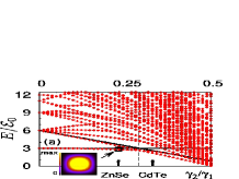
$\begin{array}[]{ccc}E\mbox{ [meV]}&g_{x}=g_{y}&g_{z}\\ 71.7&0.012&0.464\\ 71.9&0.305&0.171\\ 92.1&0.167&0.160\\ 126.1&0.274&0.237\\ 129.6&0.076&0.069\\ 130.0&0.082&0.045\\ 141.0&0.205&0.212\\ \\ 49.9&0.166&0.164\\ 52.8&0.027&0.418\\ 53.0&0.269&0.176\\ 78.5&0.162&0.169\\ 84.1&0.010&0.129\\ 84.4&0.064&0.004\\ 85.6&0.203&0.279\end{array}$

Figure 2: (Color online) (a) Levels in a cubic dot (with $\gamma_{3}=\gamma_{2}$) in units of ${\cal E}_{0}$ defined by Eq. (13). Solid lines indicate analytic result obtained when mixing between remote levels is disregarded. Note that their crossing (which we use to discern the weak and strong HH/LH splitting materials, dashed line) is very close to the actual crossing when level mixing is taken into account. Values representing ZnSe ($\bar{\gamma}_{2}/\gamma_{1}\approx 0.23$) and CdTe ($\bar{\gamma}_{2}/\gamma_{1}\approx 0.33$) QDs are indicated. Inset: squared wavefunction modulus of the ZnSe QD ground state in the $z=L/2$ section. (b) Dependence of the $g$-factors associated with the ground state Kramers doublet in a CdTe QD on its shape ($\lambda_{x}=\lambda_{y}\equiv\lambda$). Right: Energies and $g$-factors in slightly deformed QDs ($\lambda=1.01$) for the lowest 7 Kramers doublets for ZnSe and CdTe, where ${\cal E}_{0}\approx 28\ \mathrm{meV}$ and $24\ \mathrm{meV}$, respectively, for $L=8\ \mathrm{nm}$.

From Fig. 2, one may conclude that the Ising-like Hamiltonian is often an excellent approximation ($g_{x}=g_{y}=0$, as others assumeLeGall2010:PRB ; Lee2000:PRB ; Dorozhkin2003:PRB ; Katsaros2011:PRL ; LeGall2011:PRL ) for the lowest Kramers doublet. To be more specific, we now discuss materials with small and large HH/LH splitting separately. For $\gamma_{2}/\gamma_{1}<c_{R}$, the out-of-plane $g$-factor ($g_{z}$) overwhelmingly exceeds the in-plane one ($g_{x}=g_{y}$) even for minute deformation of the QD; this can be seen from the numeric ZnSe data in Fig. 2. We find $g_{z}=0.464$ and $g_{x}=g_{y}=0.012$ for $\lambda-1$ as small as $0.01$. For CdTe, which represents the other class ($\gamma_{2}/\gamma_{1}>c_{R}$), we find similar values ($g_{z}=0.418$) for the second Kramers doublet while the lowest doublet remains rather isotropic ($g_{x}=g_{y}=0.166$ and $g_{z}=0.164$). As we make the QD deformation larger, these two doublets cross, so that the ground state doublet is Ising like while the second lowest doublet remains more isotropic. This crossing occurs for $\lambda\approx 1.25$ in CdTe and data in Fig. 2(b) are only shown for $\lambda>1.25$.

We now elaborate on the properties of the low-energy sector of $\hat{H}_{2}$ (at $h=0$). Coupling between blocks of different $|m_{x}m_{y}m_{z}\rangle$ vanishes when $\gamma_{3}/\gamma_{1},\gamma_{2}/\gamma_{1}\to 0$, and Eq. (3) becomes in this limit the exact effective Hamiltonian of the lowest four levels ($m_{p}=1$ for all $p=x,y,z$). They form a quadruplet for $\lambda=1$, which splits into two doublets upon deformation of the QD; we can see it by writing

$$\langle 111|\hat{H}_{KL}|111\rangle=3{\cal E}_{0}\left[1\!\!1_{4}f(\lambda)-\hat{J}_{z}^{2}(1-\lambda^{-2})\frac{2}{3}\frac{\gamma_{2}}{\gamma_{1}}\right]$$ (15)

where $1\!\!1_{4}$ is a unit $4\times 4$ matrix and $f(\lambda)$ is a certain function with $\lim_{\lambda\to 1}f(\lambda)=1$. The lower doublet of this $4\times 4$ effective Hamiltonian has $g_{z}=1/2$ (when $\lambda>1$ and $\gamma_{2}>0$) and therefore the values of $g_{z}$ deviating from $0.5$ (appearing in Fig. 2) occur only due to admixtures from higher-orbital ($m_{p}>1$) states of LH character. Indeed, going from ZnSe to CdTe, the mixing becomes stronger and $g_{z}$ of the HH-like level drops from $0.464$ to $0.418$ ($\lambda=1.01$, numerical data in Fig. 2). While Eq. (3) may remain the effective Hamiltonian of the two doublets originating from $|m_{x}m_{y}m_{z}\rangle=|111\rangle$ even for $\gamma_{2}/\gamma_{1}>c_{R}$ (CdTe levels of $52.8$ and $53.0\ \mathrm{meV}$ in Fig. 2), for $\lambda$ close to 1, there is the more isotropic doublet on the stage ($49.9\ \mathrm{meV}$ in Fig. 2). Nevertheless, if $\lambda$ is sufficiently large, the $\hat{J}_{z}^{2}$ term in Eq. (11) will eventually dominate, it will suppress all mixing between HH and LH states and the lowest doublet will again approach $(g_{x},g_{y},g_{z})=(0,0,0.5)$ as it is shown in Fig. 2(b).

III Magnetocrystalline anisotropy energy

In analogy to the bulk systems, even cubic QDs retain anisotropies. However, these cannot be described within the previous framework: for instance, $g_{x},g_{y},g_{z}$ are all equal to $1/6$ in the cubic CdTe QD ground state hence $A=0$ in Eq. (8). One could replace $g_{ij}$ by a higher rank tensor to capture these effects, but MAE formalism of bulk magnets seems more customary and informative. Unlike the $g$-factors, MAE analysis does not invoke the concept of Kramers doublets. The zero-temperature free energy $F(\mathbf{e}_{M})$ of a magnetic QD with a single hole is now simply the lowest eigenvalue of Eq. (1) and it can be expanded in powers of $n_{j}$. The lowest terms compatible with cubic symmetry arenote3

$$F_{0}=K_{c}(n_{x}^{4}+n_{y}^{4}+n_{z}^{4})+27K_{c2}n_{x}^{2}n_{y}^{2}n_{z}^{2}.$$ (16)

For data calculated by numerically diagonalizing $\hat{H}=\hat{H}_{2}$ (model described in Sec. IIB) it turns out that Eq. (16) suffices to obtain good fits; for instance, lower solid line in Fig. 3(a) corresponds to $K_{c}=0.83\ \mathrm{meV}$ and $K_{c2}=0.075\ \mathrm{meV}$ with easy axis along $[111]$. There we have chosen Cd_1-xMn_xTe as the material, $L=16\ \mathrm{nm}$ and $h=50\ \mathrm{meV}$ which corresponds to $h=J_{pd}N_{Mn}S_{Mn}$ with $x\approx 2.3\%$ (we takematParam $|J_{pd}|=60\ \mathrm{meV\cdot nm^{3}}$, $S_{Mn}=5/2$ and $N_{Mn}=4x/a_{l}^{2}$ with CdTe lattice constant $a_{l}=0.648\ \mathrm{nm}$). Results in Fig. 3 are again subject to scaling, similar to the non-magnetic spectra in Fig. 2(a). When the material parameters (specifically, $\gamma_{2}/\gamma_{1}$ and $\gamma_{3}/\gamma_{2}$) are fixed, the spectrum of $\hat{H}_{2}$, expressed in the units of ${\cal E}_{0}$, depends on a single dimensionless parameter

$$\mbox{\v{Z}}=h/{\cal E}_{0}\equiv 2m_{0}hL^{2}/(\gamma_{1}\pi^{2}\hbar^{2}).$$ (17)

This scaling relates the spectra of e.g. cubic dots of different sizes and Mn contents (if their respective values of Ž are equal). Data in Fig. 3 therefore apply both to $x=2.3\%$ at $L=16\ \mathrm{nm}$ (if left as they are) and $x=9.2\%$ at $L=8\ \mathrm{nm}$ (if scaled by a factor of 4). It turns out that the $g$-factor analysis presented in the previous section is meaningful for $\mbox{\v{Z}}\lesssim 0.1$ while now we have stepped out of this limit. When the exchange field $h$ becomes stronger, levels cross and cease to depend linearly on $h$ as required by Eq. (6); for $\hat{H}=\hat{H}_{1}$, this is illustrated in Fig. 1(b). This limit was determined for CdTe cubic QDs but it will typically not be too different for other materials and/or aspect ratios $\lambda$ unless accidental (quasi)degeneracies occur at $\mbox{\v{Z}}=0$.

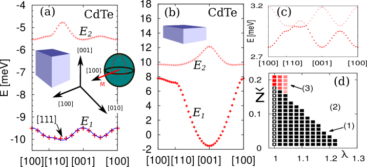
Figure 3: (Color online) Magnetocrystalline energy as a function of magnetization direction ($E_{1}$); the data labelled $E_{2}$ are explained in the text. CdTe QD with $2.3\%$ Mn (a) $16\times 16\times 16\ \mathrm{nm^{3}}$, (b) $16\times 16\times 8\ \mathrm{nm^{3}}$. (c) Fictitious material with parameters described in the text; note that the sign of $K_{c}$ implied by Eq. (16) has changed compared to (a,b). (d) Color-coded easy axis positions for CdTe QDs as a function of aspect ratio ($\lambda$) and effective exchange splitting Ž. Black squares (1) indicate easy plane perpendicular to $z$-direction, hollow squares denote an isotropic magnet; white region (2) corresponds to easy-axis [001]; red squares (3) denote systems with [111] easy axis which gradually shifts towards [001] with increasing $\lambda$. This plot is universal as far as $L$ is concerned.

		cubic			deformed
		ZnSe	CdTe		ZnSe		CdTe
$h$ [meV]	Ž	$K_{c}$	$K_{c}$		$K_{c}$	$K_{u}$	$K_{c}$	$K_{u}$
10	0.55	0.11	0.24		0.23	-3.79	0.35	-3.90
20	1.1	0.20	0.43		0.36	-5.52	0.62	-6.21
30	1.7	0.28	0.59		0.44	-6.29	0.83	-7.59
40	2.2	0.35	0.71		0.50	-6.72	1.01	-8.56
50	2.8	0.41	0.83		0.56	-7.01	1.16	-9.30

Table 1: Magnetic anisotropy constants (in meV) for a $16\times 16\times 16\ \mathrm{nm^{3}}$ (cubic) and $16\times 16\times 8\ \mathrm{nm^{3}}$ (deformed) ZnSe and CdTe magnetic QD as a function of exchange splitting (or dimensionless parameter Ž as for CdTe).

MAE shown in Fig. 3 describe systems well beyond this limit of small Ž (linear regime). We first focus on a perfectly cubic CdTe QD where there are no anisotropies in the linear regime. As already mentioned, the lowest energy hole state in Fig. 3(a) exhibits a [111] easy axis with $K_{c}=0.83\ \mathrm{meV}$ at $L=16\ \mathrm{nm}$ and $h=50\ \mathrm{meV}$, i.e. $\mbox{\v{Z}}\approx 2.8$, (this corresponds to a realistic $x\approx 2.3\%$ Mn doping). In bulk DMSs, [111] would be an unusual magnetic easy axis directionZemen2009:PRB and we surmise that the reason for this is that for instance in (Ga,Mn)As grown on a GaAs substrate, there is a sizable compressive strain which prefers either parallel or perpendicular orientation of $\mathbf{e}_{M}$ with respect to the growth axis.

We note that in a QD containing two holes (closed-shell systemOszwaldowski2011:PRL ) the anisotropies will also be present and they will be different from the single-hole case. Free energy, taken as a sum, $F_{0}(\mathbf{e}_{M})=E_{1}+E_{2}$, of the lowest two single-hole states [shown e.g. in Fig. 3(a)], is not a constant independent of $\mathbf{e}_{M}$ as one could naively expect. This intuition reflects $\hat{H}_{\rm eff}$ in Eq. (6) where the two hole states have opposite spin (hence their energies add up to zero). Once we leave the linear regime ($\mbox{\v{Z}}\gtrsim 0.1$), $\hat{H}_{\rm eff}$ ceases to be a good approximation. Qualitatively, the same behaviour is found for ZnSe (not shown), a smaller value of $K_{c}=0.41\ \mathrm{meV}$ is accounted for by the smaller HH/LH splitting. The value of this constant is a complicated function of system parameters and it can even change sign as shown in Fig. 3(c) where $K_{c}=-0.63\ \mathrm{meV}$. Parameters used in this figure ($\gamma_{1}/\gamma_{2}/\gamma_{3}=4.0/1.5/1.6$ and $h=20\ \mathrm{meV}$) do not strictly correspond to published values of any semiconductor but they can be viewed as reasonable given the uncertainty in experimental determination of the Luttinger parameters. Dependence of the anisotropy constants for ZnSe and CdTe QDs on $h$ is summarized in Tab. 1.

Let us now return to non-cubic QDs. As already explained, the sizable $g$-factor anisotropies shown in Fig. 2(b), relevant to the case of weak magnetism ($\mbox{\v{Z}}\ll 1$), translate into an additional term $AF_{1}=K_{u}n_{z}^{2}$ in the free energy of Eq. (2) where $K_{u}=-kA$ up to linear order in $\mbox{\v{Z}}\propto k$. Typically, $K_{u}$ exceeds $K_{c}$ already for small QD deformation ($\lambda$ slightly over one) and the data in Fig. 3(b) imply $K_{u}$ almost an order of magnitude larger than $K_{c}$ for $\lambda=2$ (see also data in Fig. 2 where $g_{z}\gg g_{x}$). Regardless of the contributions to $K_{u}$ of higher order in Ž, data in Tab. 1 imply an out-of-plane easy axis (in the [001] direction) as it is the case in QWs. However, upon deforming of a QD the easy axis does not abruptly jump from [111] to [001] but smoothly interpolates between these two directions. Similar effect, easy axis shifting as a function of some system parameter, is also known in bulk DMS [(Ga,Mn)As epilayers in particular, see Fig. 8 in Ref. Zemen2009:PRB, ]. Easy axes as a function of QD shape (oblate dots, $\lambda>1$) and effective exchange splitting Ž are summarized in Fig. 3(d) and the mentioned gradual shift of easy axis is indicated by shading between regions (3) and (2) (easy axes $[111]$ and $[001]$, respectively). On the other hand, the easy axis position changes abruptly between (1) and (3) or (1) and (2); region (1) corresponds to easy axis in the plane perpendicular to $[001]$ (with anisotropies within this plane being very small). The abrupt changes reflect ground state crossings, such as the one with $\lambda$ described below Eq. (14), while the gradual ones stem from level mixing caused by $\hat{H}_{ex}$.

Finally, we comment on MA in QDs occupied by more than one hole. As already mentioned above, one possible approach is to discuss open-shell and closed-shell systems separately. This notion is based on the concept of the QD being an artificial atom whose levels are organized into shells comprising of spin-up and spin-down orbitals. Whenever a shell is completely filled (closed), the numbers of spin-up and spin-down carriers are equal hence their total spin is zero. If the QD is magnetically doped, no magnetic ordering is expected and also no MA. However, strong SO coupling puts this concept into question since it mixes different shells and also invalidates the spin-up and down labels of individual orbitals. The MA as a function of particle number $N_{p}$ strongly varies, both quantitatively and qualitatively. By comparing the $N_{p}=1$ and $N_{p}=2$ cases of a cubic CdTe QD, that is $F_{0}(\mathbf{e}_{M})=E_{1}$ and $F_{0}(\mathbf{e}_{M})=E_{1}+E_{2}$ of Fig. 3(a), we find that while the easy axis $[111]$ in the former case is relatively ‘soft’ (energy difference between $\mathbf{e}_{M}||[111]$ and $[110]$ is ‘only’ $\approx 0.1\ \mathrm{meV}$), the QD with two holes has a ‘robust’ easy axis $[110]$ and the corresponding minimum in $F_{0}(\mathbf{e}_{M})$ is as deep as $0.3\ \mathrm{meV}$. MA as a function of $N_{p}$ displays rich behavior and one can therefore envision control of nanomagnetism by electrostatic gating, illumination (used to photoinduce carriers) and possibly also temperature, known to alter the magnetic ordering in the bulk-like structures.Zutic2004:RMP ; igor

IV Conclusions

We have discussed two approaches to magnetic anisotropies in quantum dots (QDs) described by a generic model in Eq. (1). An effective Hamiltonian for individual Kramers doublets allows to express the energetics of a magnetically doped QD in terms of only three parameters (anisotropic $g$-factor) if the exchange splitting due to the magnetic ions is relatively small. On the other hand, if the exchange splitting is large or the QD’s symmetry is too high, the symmetry-based expansion of the magnetocrystalline energy in powers of the direction cosines of magnetization may in principle contain infinitely many terms (each of them quantified by one parameter). Focusing on manganese-doped semiconductor QDs, we find that only first few terms are appreciable, present their values and show in Fig. 3(d) a diagram of magnetic anisotropies in the QD parameter space. While we focus on a relatively small parameter range in that diagram, and the barriers between individual free energy minima are relatively low, it demonstrates that the QDs may have rich magnetic anisotropies. In spintronics,Zutic2004:RMP ; Fabian2007:APS ; Tarucha2006:bookCh these systems could thus enable confinement-controlled multi-level logic. Our results provide a starting point for further studies of nanoscale magnetism in QDs. Such studies could relax the mean-field approximation, include multiple-carrier states,fewElectrons ; Cheng2009:PRB or the effect of strain.

Appendix A

The downfolding of $\hat{H}_{QD}+\hat{H}_{ex}$ to $\hat{H}_{\rm eff}$ is indeed possible for the two example systems discussed in Sec. IIA and IIB. To prove this, we first transform the basis $|K_{1}\rangle,|K_{2}\rangle$ to $|K_{1}^{\prime}\rangle,|K_{2}^{\prime}\rangle$ where $\tilde{t}_{z}$ of Eq. (7) is diagonal and then verify that the diagonal elements of $\tilde{t}_{x}$ and $\tilde{t}_{y}$ vanish. This procedure has to be applied to each Kramers doublet of interest. In the case of $\hat{H}_{1}$ in Eq. (3), this is done simply by construction (e.g. $|K_{1}^{\prime}\rangle,|K_{2}^{\prime}\rangle$ for the upper doublet in Fig. 1(a) is just $|J_{z}=3/2\rangle,|J_{z}=-3/2\rangle$). In the model described by $\hat{H}_{2}$, one can split the Hilbert space into two disjunct subspaces $\mathscr{H}_{1}$, $\mathscr{H}_{2}$ and the above assertion can be shown to hold if $|K_{1}^{\prime}\rangle\in\mathscr{H}_{1}$ and $|K_{2}^{\prime}\rangle\in\mathscr{H}_{2}$. (The decomposition $\mathscr{H}_{1}\oplus\mathscr{H}_{1}$ relies on $\hat{H}_{ex}$ being independent of space coordinates; relaxing the mean-field treatment of Mn magnetic moments thus introduces corrections to $\hat{H}_{\mathrm{eff}}$.) Finally, one adjusts the relative phase between $|K_{1}^{\prime}\rangle$ and $|K_{2}^{\prime}\rangle$, so that the matrix $\tilde{t}_{x}$ is real and $\tilde{t}_{y}$ purely imaginary.

Appendix B

This Appendix explains the relation between the anisotropic $g$-factors and Eq. (2). The eigenvalues of $\hat{H}_{\rm eff}$ are two numbers of equal magnitude and opposite sign, the lower of which is

$$-h\sqrt{n_{x}^{2}g_{x}^{2}+n_{y}^{2}g_{y}^{2}+n_{z}^{2}g_{z}^{2}}.$$ (18)

Let us consider for example single hole in a cuboid QD of dimensions $\lambda L\times\lambda L\times L$ (such as it corresponds to data in Fig. 2) so that $g_{x}=g_{y}$. Expression (18) which now equals $F(\mathbf{e}_{M})$ can be rewritten as

$$-\frac{h\sqrt{g_{x}^{2}+g_{z}^{2}}}{\sqrt{2}}\sqrt{1+\frac{g_{z}^{2}-g_{x}^{2}}{g_{z}^{2}+g_{x}^{2}}(n_{z}^{2}-n_{x}^{2}-n_{y}^{2})}$$ (19)

and developped in terms of a small parameter $A=(g_{z}^{2}-g_{x}^{2})/(g_{z}^{2}+g_{x}^{2})$ which quantifies the QD asymmetry as

$${\textstyle-k(1-\frac{1}{2}A)-Akn_{z}^{2}+\frac{1}{8}A^{2}k(2n_{z}^{2}-1)^{2}+\ldots}$$ (20)

where $k=h\sqrt{(g_{x}^{2}+g_{z}^{2})/2}$. The first term does not depend on the magnetization direction, hence it can be disregarded for the purposes of magnetic anisotropy analysis.

Appendix C

We derive Eq. (14) in this Appendix and discuss the details of the model considered in Sec. IIB. Energies $E/{\cal E}_{0}$ in Fig. 2(a) are calculated by numerical diagonalization of $\hat{H}_{2}$ with $h=0$, a matrix constructed of $4\times 4$ blocks $\langle m_{x}m_{y}m_{z}|\hat{H}_{KL}|m_{x}^{\prime}m_{y}^{\prime}m_{z}^{\prime}\rangle/{\cal E}_{0}$ introduced at the beginning of Sec. IIB. The basis of $\hat{H}_{QD}$ consists thus of direct product states $|m_{x}m_{y}m_{z}\rangle\otimes|J_{z}\rangle$ where $|J_{z}\rangle$ are the four-spinors of total angular momentum $J=3/2$ which are eigenstates to $\hat{J}_{z}$. For practical purposes, we cut-off the basis by $m_{x},m_{y},m_{z}\leq 6$, resulting in $\hat{H}_{QD}$ of dimension 864. Eigenvalues are typically converged to better than $0.1\ \mathrm{meV}$ for this cut-off.

The matrix $\hat{H}_{QD}/{\cal E}_{0}$ is block-diagonal for $\gamma_{2}=\gamma_{3}=0$ and the block $m_{x},m_{y},m_{z}$ has a four-fold degenerate eigenvalue

$$(m_{x}/\lambda_{x})^{2}+(m_{y}/\lambda_{y})^{2}+m_{z}^{2}.$$ (21)

Dimensionless energies on the left of Fig. 2(a) correspond to $\lambda_{x}=\lambda_{y}=1$ and are hence integers. The lowest level $E/{\cal E}_{0}=3$ belongs to $(m_{x},m_{y},m_{z})=(1,1,1)$ while the first excited state $E/{\cal E}_{0}=6$ entails an additional threefold geometric degeneracy corresponding to orbital states $(1,1,2)$, $(1,2,1)$ and $(2,1,1)$; the $E/{\cal E}_{0}=6$ level for $\gamma_{2}=\gamma_{3}=0$ is thus twelve-fold degenerate.

Next, we can treat the HH-LH splitting as a perturbation when $\gamma_{2}$ and $\gamma_{3}$ are turned on. In the lowest order, mixing between different $(m_{x},m_{y},m_{z})$ blocks can be neglected except for the case when their energies were equal at $\gamma_{2}=\gamma_{3}=0$ as in the case of the three blocks of the $E/{\cal E}_{0}=6$ level. With coupling to the remote levels disregarded, we are left with a $12\times 12$ matrix in this case which can be diagonalized analytically. It turns out to have two four-fold degenerate eigenvalues

$$E_{4}^{\pm}/{\cal E}_{0}=6+\frac{64}{3\pi^{2}}\frac{\gamma_{2}}{\gamma_{1}}\left(s\pm\sqrt{s^{2}+\frac{81\pi^{4}}{1024}}\right)$$ (22)

and two two-fold degenerate ones

$$E_{2}^{\pm}/{\cal E}_{0}=6-\frac{128}{3\pi^{2}}\frac{\gamma_{2}}{\gamma_{1}}\left(s\mp\frac{9\pi^{2}}{64}\right).$$ (23)

The lowest of these four energies is $E_{2}^{-}$ and it is shown in Fig. 2(a) for $s\equiv\gamma_{3}/\gamma_{2}=1$ as a solid line which crosses the horizontal line $E/{\cal E}_{0}=3$ corresponding to the $(m_{x},m_{y},m_{z})=(1,1,1)$ quadruplet which does not shift in energy to the first order of this perturbation analysis. Eq. (14) is the solution of $E_{2}^{-}=3{\cal E}_{0}$ for $\gamma_{2}/\gamma_{1}$ under the assumption $s=1$. Such level crossing (as a function of $\gamma_{2}/\gamma_{1}$) is genuinely due to the confinement and no level crossings occur in in bulk as long as $0<\gamma_{2}/\gamma_{1}<1/2$.

References

- (1) U. Welp, V. K. Vlasko-Vlasov, X. Liu, J. K. Furdyna, and T. Wojtowicz, Phys. Rev. Lett. 90, 167206 (2003).
- (2) X. Liu, Y. Sasaki and J. K. Furdyna, Phys. Rev. B 67, 205204 (2003).
- (3) J. Fernández-Rossier and R. Aguado in Handbook of Spin Transport and Magnetism, edited by E. Y. Tsymbal and I. Žutić (CRC Press, New York, 2012).
- (4) D. R. Yakovlev and W. Ossau in Introduction to the Physics of Diluted Magnetic Semiconductors, edited by J. Kossut and J.A. Gaj (Springer, New York, 2010).
- (5) R. Beaulac, L. Schneider, P. I. Archer, G. Bacher, and D. R. Gamelin, Science 325, 973 (2009).
- (6) I. R. Sellers, R. Oszwałdowski, V. R. Whiteside, M. Eginligil, A. Petrou, I. Žutić, W.-C. Chou, W. C. Fan, A. G. Petukhov, S. J. Kim, A. N. Cartwright, and B. D. McCombe, Phys. Rev. B 82, 195320 (2010).
- (7) F. Henneberger and J. Puls, in Introduction to the Physics of Diluted Magnetic Semiconductors, edited by J. Kossut and J.A. Gaj (Springer, New York, 2010).
- (8) R. M. Abolfath, A. G. Petukhov, and I. Žutić, Phys. Rev. Lett. 101, 207202 (2008).
- (9) A. O. Govorov, Phys. Rev. B 72, 075359 (2005); A. O. Govorov, ibid. 72, 075358 (2005).
- (10) D. A. Bussian, S. A. Crooker, Ming Yin, M. Brynda, A. L. Efros, and V. I. Klimov, Nature Mat. 8, 35 (2009).
- (11) R. Oszwałdowski, I. Žutić, and A. G. Petukhov, Phys. Rev. Lett. 106, 177201 (2011).
- (12) S. T. Ochsenbein, Yong Feng, K. M. Whitaker, E. Badaeva, W. K. Liu, X. Li, and D. R. Gamelin Nature Nanotechnology 4, 681 (2009); I. Žutić and A. G. Petukhov, ibid. 4, 623 (2009).
- (13) H. Enaya, Y. G. Semenov, J. M. Zavada, and K. W. Kim, J. Appl. Phys. 104, 084306 (2008).
- (14) C. Le Gall, R. S. Kolodka, C. L. Cao, H. Boukari, H. Mariette, J. Fernández-Rossier, and L. Besombes, Phys. Rev. B 81, 245315 (2010).
- (15) J. Zemen, K. Olejník, J. Kučera, and T. Jungwirth, Phys. Rev. B 80, 155203 (2009).
- (16) L. Dreher, D. Donhauser, J. Daeubler, M. Glunk, C. Rapp, W. Schoch, R. Sauer, and W. Limmer, Phys. Rev. B 81, 245202 (2010).
- (17) T. L. Linnik, A. V. Scherbakov, D. R. Yakovlev, X. Liu, J. K. Furdyna, M. Bayer, arXiv1111.4043 (2011).
- (18) I. Žutić, J. Fabian and S. Das Sarma, Rev. Mod. Phys. 76, 323 (2004).
- (19) J. Fabian, A. Matos-Abiague, Ch. Ertler, P. Stano, and I. Žutić, acta phys. slov. 57, 565 (2007).
- (20) S. D. Bader, Rev. Mod. Phys. 78, 1 (2006).
- (21) J. Fernández-Rossier and R. Aguado, Phys. Rev. Lett. 98, 106805 (2007).
- (22) S. J. Cheng, Phys. Rev. B 79, 245301 (2009)
- (23) F. V. Kyrychenko and J. Kossut, Phys. Rev. B 70, 205317 (2004).
- (24) B. Lee, T. Jungwirth, and A. H. MacDonald, Phys. Rev. B 61, 15606 (2000).
- (25) I. A. Merkulov and K. V. Kavokin, Phys. Rev. B 52, 1751 (1995).
- (26) C. E. Pryor and M. E. Flatté, Phys. Rev. Lett. 96, 026804 (2006).
- (27) A. K. Bhattacharjee, Phys. Rev. B 76, 075305 (2007).
- (28) Magnetostatic shape anisotropy will compete with MAE as soon as the QD is not perfectly cubic. To estimate the shape anisotropy energy, we use parameters similar to those discussed in Sec. III. Taking of Eq. (17) and as a reference point (in-plane magnetization in a QD is preferred to by ), magnetostatic shape anisotropyZemen2009:PRB does not reach even .
- (29) See Sec. III.A of Ref. Fabian2007:APS, for an introduction to Kramers doublets. Note that multiple doublets may sometimes be degenerate either because of symmetry or by accident.
- (30) L. Besombes, Y. Léger, L. Maingault, D. Ferrand, H. Mariette, and J. Cibert, Phys. Rev. Lett. 93, 207403 (2004); L. Besombes, Y. Léger, L. Maingault, D. Ferrand, H. Mariette, and J. Cibert, Phys. Rev. B 71, 161307 (2005).
- (31) I. A. Merkulov and A. V. Rodina in Introduction to the Physics of Diluted Magnetic Semiconductors, edited by J. Kossut and J. A. Gaj (Springer, New York, 2010).
- (32) A. G. Petukhov, W. R. L. Lambrecht and B. Segall, Phys. Rev. B 53, 3646 (1996).
- (33) P. S. Dorozhkin, A. V. Chernenko, V. D. Kulakovskii, A. S. Brichkin, A. A. Maksimov, H. Schoemig, G. Bacher, A. Forchel, S. Lee, M. Dobrowolska, and J. K. Furdyna, Phys. Rev. B 68, 195313 (2003).
- (34) G. Katsaros, V. N. Golovach, P. Spathis, N. Ares, M. Stoffel, F. Fournel, O. G. Schmidt, L. I. Glazman, and S. De Franceschi, Phys. Rev. Lett. 107, 246601 (2011).
- (35) C. Le Gall, A. Brunetti, H. Boukari, and L. Besombes, Phys. Rev. Lett. 107, 057401 (2011).
- (36) Material parameters were taken from the following sources. CdTe: from Ref. Friedrich1994:JPCM, , from Ref. Kyrychenko2004:PRB, . ZnSe: from Ref. Venghaus1979:PRB, .
- (37) T. Friedrich, J. Kraus, M. Meininger, G. Schaack, W. O. G. Schmitt, J. Phys.: Cond. Mat. 6, 4307 (1994).
- (38) H. Venghaus, Phys. Rev. B 19, 3071 (1979).
- (39) We basically follow the conventions of Eq. (12) in Ref. Zemen2009:PRB, with aesthetically more pleasing . equals (Eq. (2) of Ref. Linnik2011:arxiv, ) or (Eq. (21) of Ref. Dreher2010:PRB, ).
- (40) T. Jungwirth, Jairo Sinova, J. Mašek, J. Kučera, and A. H. MacDonald, Rev. Mod. Phys. 78, 809 (2006); H. Ohno, D. Chiba, F. Matsukura, T. Omiya, E. Abe, T. Dietl, Y. Ohno, and K. Ohtani, Nature 408, 944 (2000); S. Koshihara, A. Oiwa, M. Hirasawa, S. Katsumoto, Y. Iye, C. Urano, H. Takagi, and H. Munekata, Phys. Rev. Lett. 78, 4617 (1997); A. G. Petukhov, I. Žutić and S. C. Erwin, Phys. Rev. Lett. 99, 257202 (2007); M. J. Calderón and S. Das Sarma, Phys. Rev. B 75, 235203 (2007); V. Krivoruchko, V. Tarenkov, D. Varyukhin, A. D’yachenko, O. Pashkova, and V. Ivanov, J. Magn. Magn. Mater 322, 915 (2010).
- (41) Concepts in Spin Electronics, edited by S. Maekawa (Oxford University Press, Oxford, 2006).
- (42) N. T. T. Nguyen and F. M. Peeters Phys. Rev. B 80, 115335 (2009); F. Qu and P. Hawrylak, Phys. Rev. Lett. 96, 157201 (2006).