Synchronization in Scale Free networks with degree correlation

Abstract

In this paper we study a model of synchronization process on scale free networks with degree-degree correlations. This model was already studied on this kind of networks without correlations by Pastore y Piontti et al., Phys. Rev. E 76, 046117 (2007). Here, we study the effects of the degree-degree correlation on the behavior of the load fluctuations $W_{s}$ in the steady state. We found that for assortative networks there exist a specific correlation where the system is optimal synchronized. In addition, we found that close to this optimally value the fluctuations does not depend on the system size and therefore the system becomes fully scalable. This result could be very important for some technological applications. On the other hand, far from the optimal correlation, $W_{s}$ scales logarithmically with the system size.

I Introduction

In the last decades the study of complex networks received much attention because many real processes work over these kind of structures. Historically, the research was mainly focused on how the topology affects processes such as epidemic spreadings Pastorras_PRL_2001 , traffic flow Lopez_transport ; zhenhua , cascading failures Motter_prl and synchronization problems Jost-prl ; Korniss07 . Many real networks have structures characterized by a degree distribution $P(k)\sim k^{-\lambda}$ known as scale free (SF), where $k$ is the degree or number of connections that a node can have and $k_{max}\geq k\geq k_{min}$, where $k_{max}$ is the maximum degree, $k_{min}$ the minimum degree and $\lambda$ measure the broadness of the distribution Barabasi_sf . In synchronization process it is customary to study the fluctuations $W=\left\{1/N\sum_{i=1}^{N}(h_{i}-\langle h\rangle)^{2}\right\}^{1/2}$ of some scalar field $h$, where $h_{i}$ with $i=1,N$ represent the scalar field on node $i$, $\langle h\rangle$ is the mean value, $N$ is the system size and $\{.\}$ denotes an average over network configurations. These kind of problems are very important in many real situations such as supply-chain networks based on electronic transactions Nagurney , brain networks JWScanell and networks of coupled populations in correlated epidemic outbreaks eubank_2004 . Pastore y Piontti et. al anita studied a model of surface relaxation with non-conservative noise that allows to balance the load and reduce the fluctuations (synchronize) of the scalar fields on SF networks without degree correlation. However real networks are correlated in nature, and there should be a reason for this feature. One reason could be to enhance some process such as the transport and the synchronization through them. The degree-degree correlation of a network can be measured using the Pearson’s coefficient given by newman

$$r=\frac{M^{-1}\sum_{i=1}^{M}j_{i}k_{i}-\left[M^{-1}\sum_{i=1}^{M}\frac{1}{2}(j_{i}+k_{i})\right]^{2}}{M^{-1}\sum_{i=1}^{M}\frac{1}{2}(j_{i}^{2}+k_{i}^{2})-\left[M^{-1}\sum_{i=1}^{M}\frac{1}{2}(j_{i}+k_{i})\right]^{2}}\ ,$$ (1)

where $M$ is the number of edges of the network and $j_{i}$ and $k_{i}$ are the degree of the nodes of the edge $i$. This coefficient only can takes values in the interval $[-1,1]$: if $r<0$ the network is called disassortative (nodes with low degree tend to connect with highly connected nodes) while for $r>0$ the network is called assortative (nodes tend to connect with others with the similar degrees). When $r=0$ the network is uncorrelated. As observed in many other works the degree-degree correlation affects considerably the processes that occur on top of them noh ; ana2 ; sorrentino .

In this paper we study the effects of the degree-degree correlation on the behavior of the fluctuations in the steady state $W_{s}$ of SF correlated networks with $\lambda<3$ for the model of surface relaxation to the minimum (SRM) family used by Pastore y Piontti et. al anita in uncorrelated networks. To study the fluctuations we map the process with a problem of a non-equilibrium surface growth EW , where the scalar field $h_{i}\equiv h_{i}(t)$ represents the interface height at each node $i$ at time $t$. We found that for every $\lambda<3$ there exist a value of the correlation for which the fluctuations are minimized, i.e, that optimizes the synchronization. Close to and at the “optimal” correlation the fluctuations does not depend on $N$, but for other correlations the fluctuations diverges logarithmically with $N$.

II Model and Simulation

To construct the networks we use the configurational model (CM) MolloyCorrelation with a degree cutoff $k_{max}=N^{1/2}$ for $\lambda<3$ in order to uncorrelate the original network correlacion . Then, we choose two links at random and with probability $p$ we connect the nodes with higher degree between them and the two with smaller degree to each other to obtain $r>0$. For $r<0$, we connect with probability $p$ the node with highest degree with the one with lowest degree and the other two between them. In both cases we do not allow self loops or multiple connections. It is known that algorithms that generate clustering (the probability that two connected nodes have another neighbor in common) produce degree-degree correlation, but the algorithm used here produce degree-degree correlation without introducing clustering Newman-Miller . In this way, we can study the effects of the degree-degree correlation on SF networks isolating them from clustering effects. A side effect of this algorithm is that for SF networks the range of Pearson’s coefficient that can be generated cannot span the total domain $r\in[-1,1]$. Nevertheless, the range that can be obtained is enough to observe how change the scaling of the fluctuations with the system size when correlations are introduced. For all the results in this work we use $k_{min}=2$ in order to ensure that the network is fully connected cohen . We present the results for $\lambda=2.5$ but we checked that for $2<\lambda<3$ they are qualitatively the same. The reason to investigate only $2<\lambda<3$ is because almost all the real SF networks fall in this range of values of $\lambda$.

In the SRM model anita ; family , at each time step a node $i$ is chosen to evolve with probability $1/N$. Then, if we denote by $v_{i}$ the nearest neighbor nodes of $i$, the growing rules are: (1) if $h_{i}\leq h_{j}$ $\forall j\in v_{i}$ $\Rightarrow h_{i}=h_{i}+1$, else (2) if $h_{j}<h_{n}$ $\forall n\not=j\in v_{i}$ $\Rightarrow h_{j}=h_{j}+1$. For the simulations we start with an initial configuration of $\{h_{i}\}$ randomly distributed in the interval $[0,1]$.

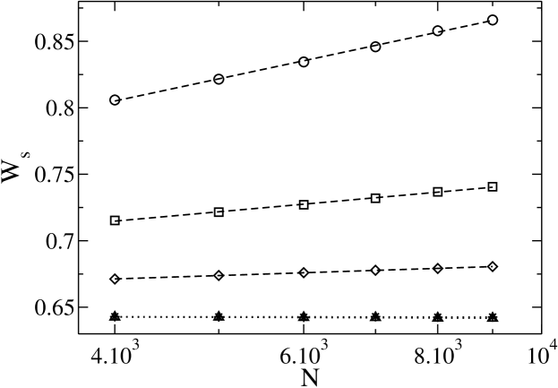
Figure 1: $W_{s}$ as a function of $N$ in log-linear scale for $\lambda=\ 2.5$ and $k_{min}=2$ for $r=-0.237$ ($\bigcirc$), $-0.05$ ($\Box$), $0.103$ ($\diamond$), $r_{min}=0.335$ ($\bigtriangleup$) and 0.386 ($\star$). The dashed lines represent a logarithmic fitting and the dotted lines a linear fitting.

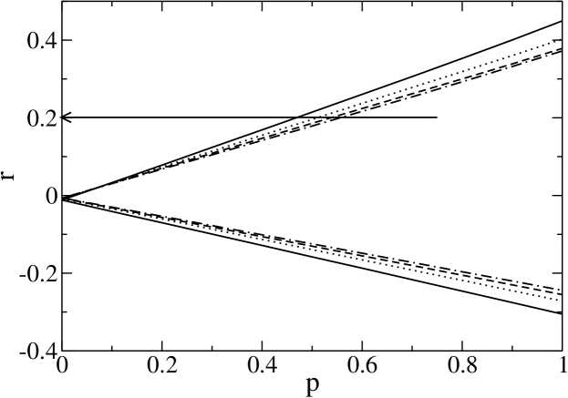
Figure 2: $r$ as a function of $p$ for $\lambda=\ 2.5$ and $k_{min}=2$ for $N=1000$ (straight line), $3000$ (dotted line), $5000$ (dashed line) and $7000$ (dot-dashed line). The straight horizontal line with the arrow indicate the values of $p$ used for $r=0.2$.

In Fig. 1 we show, in log-linear scale, $W_{s}$ as a function of $N$ for different values of $r$ for $\lambda=2.5$. We can see that for some values of $r$, $W_{s}$ has a logarithmic divergence with $N$ while for other values of $r$, $W_{s}$ does not depend or has a weakly dependence on $N$. This change of behavior means that the scaling of the fluctuations not only depends on $\lambda$ anita , it also depends on the correlation of the network. These results are in agreement with Ref. anita , where for uncorrelated, or slightly disassortative networks, $W_{s}$ scales as $\ln N$ for $\lambda<3$ ($r=-0.05$ in Fig. 1). Notice that the relation between $r$ and $p$ has finite size effects (See Fig. 2). For this reason if we want to fix $r$ we must select different values of $p$ for each system size.

In Fig. 3 we plot $W_{s}^{2}$ as a function of $r$ for $N=5000$. Each data point was obtained from the linear fitting of $W^{2}(t)$ in the saturated regime for each $r$ value for $3000$ realizations, a task of very time consuming. We can see that there is a positive value $r=r_{min}$ that minimizes (optimizes) the fluctuations. In the inset figure we show $r_{min}$ as a function of $N$. We can see that for large system size ($N\gtrsim 3000$) the optimal correlation is independent of $N$. The dashed line represent the linear fitting of $r_{min}$ for large $N$, from where we found that $r_{min}\approx 0.335$ for $\lambda=2.5$. This means that for the optimal correlation the fluctuations in the steady state do not depend on the system size. This is an important result because for $r$ close to $r_{min}$ the whole system is scalable with $N$. As an example, suppose that we have a cluster of computers connected as a SF network with $r\approx r_{min}$, and that the excess of load of the cluster of computers is sent to the first neighbors in one time step as in our model. In the optimal correlation, as we show, the fluctuations are independent of $N$, so we could increase the number of computers in our system as much as we want without losing its synchronization.

In order to explain this behavior we compute the local contribution to the fluctuations due to all nodes with degree $k$ in the steady state, given by

$$W_{k}^{2}=\frac{1}{NP(k)}\sum_{i=1,k_{i}=k}^{N}W_{i}^{2}\ ,$$

and therefore the total fluctuation can be computed as

$$W_{s}^{2}=\sum_{k=k_{min}}^{k_{max}}P(k)W_{k}^{2}\ .$$ (2)

In Fig. 4 a) we show $W_{k}^{2}$ as a function of $k$ for $\lambda=$ $2.5$, $N=5000$ and different values of $r$. We can see that for nodes with high degree, $W_{k}^{2}$ decreases as $r$ increases. This is due to the fact that when $r$ increases nodes tend to connect with others with similar connectivities and since the high degree nodes are few and tightly packed, the one step relaxation is enough for even out all their heights, balancing better the load and enhancing the synchronization. On the other hand, for low degree nodes we observe that $W_{k}^{2}$ has a minimum for the optimal correlation, as shown in Fig. 4 b). In SF networks the majority of the nodes have low connectivities and if $r>0$ the average distance between those nodes becomes bigger that one noh . As the relaxation is only to first neighbors, different parts of those chains will have very different heights. As a consequence, for some values of $r>0$ not all the low degree nodes will be completely synchronized between them. For this reason the optimal correlation is positive and smaller than one since low degree nodes are connected to some nodes with high degree allowing to speed up the relaxation and smoothing out the interface among them.

In order to prove this, in Fig. 5 we plot the cumulative

$$W_{c}^{2}(k)=\sum_{k^{{}^{\prime}}=kmin}^{k}W_{k^{{}^{\prime}}}^{2}P(k^{{}^{\prime}})\ .$$ (3)

As we can see from the plot, as $r$ increases the contribution to $W_{s}$ of high degree nodes decreases, being the main contribution to the fluctuations due to low degree nodes for positive $r$ and the smaller for $r_{min}$. This is why the global fluctuations is minimal in the optimal correlation. Also from the same plot we can understand why close to the optimal correlation the system does not depend on $N$. For $k>k^{*}$, Eq. (3) can be rewritten as

$$W_{c}^{2}(k)=W_{c}^{2}(k^{*})+\sum_{k^{{}^{\prime}}={k^{*}+1}}^{k}W_{k^{{}^{\prime}}}^{2}P(k^{{}^{\prime}})\ ,$$

where $k^{*}$ is the upper value of $k$ that separate two different regimes for $W_{c}^{2}(k)$. The second term can be replaced by $A(k)$, where

$$A(k)\sim\left\{\begin{array}[]{ll}\ln k,&\hbox{$r<r_{min}$ and $r>r_{min}$\ ;}\\ \mbox{const.},&\hbox{$r\simeq r_{min}$\ .}\end{array}\right.$$ (6)

Then Eq. (2) is given by

$$W_{s}^{2}=W_{c}^{2}(k_{max})\ ,$$

where $k_{max}=\sqrt{N}$. Using Eq. (6)

$$W_{s}^{2}\sim\left\{\begin{array}[]{ll}\ln k_{max}\sim\ln\sqrt{N}\sim\ln N,&\hbox{$r<r_{min}$ and $r>r_{min}$\ ;}\\ \mbox{const.},&\hbox{$r\approx r_{min}$\ .}\end{array}\right.$$ (9)

The logarithmic divergence far from the optimal correlation is a consequence of that the contribution of high degree nodes cannot be disregarded. However in $r=r_{min}$ only the low degree nodes contribute to the global fluctuations of the system allowing the scalability with the system size.

III Summary

In this paper we study the effects of degree degree correlations on the behavior of the fluctuations $W_{s}$ for the SRM model in SF networks with $2<\lambda<3$. We found that there exist an optimal value of the Pearson’s coefficient $0<r_{min}<1$ (assortative networks) where the system is optimal synchronized. We also found that for values close to $r_{min}$ the fluctuations does not depend on $N$, i.e, it is scalable. Moreover for $r<r_{min}$ and $r>r_{min}$ the fluctuations diverge as a logarithmically with the system size $N$. Then the scaling behavior of $W_{s}$ with the system size depend strongly on the correlation of the network.

The optimal synchronization found for assortative networks is in our model a topological effect due to the correlations. This is an unexpected result because in many researches it was found that disassortative networks (communication networks) are better for transport ana2 and to synchronize oscillators sorrentino .

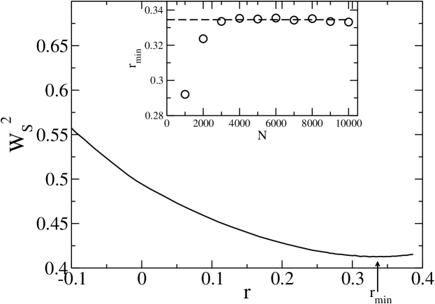
Figure 3: $W_{s}^{2}$ as a function of $r$ for $\lambda=2.5$ and $N=5000$. The arrow indicate the position $r_{min}$. In the inset figures we plot $r_{min}$ as a function of $N$ in symbols. The dashed line represent the linear fitting in the region where $r_{min}$ is independent of $N$: $r_{min}=0.335$ for $\lambda=2.5$. The averages were done over $3000$ realizations.

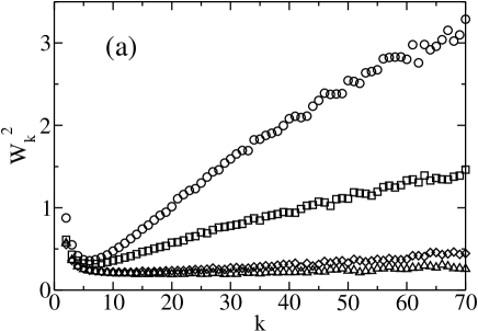
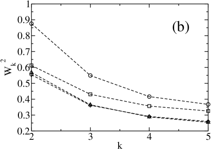
Figure 4: $W_{k}^{2}$ vs $k$ for $\lambda=\ 2.5$, $r=-0.255$ ($\circ$), $-7.10^{-03}$ ($\Box$), $0.335$ ($r_{min}$) ($\diamond$) and $0.386$ ($\bigtriangleup$) b) An amplification of a) for low degree nodes. The dashed lines are used as guides. All these results are for $N=5000$ and $5000$ realizations of the networks.

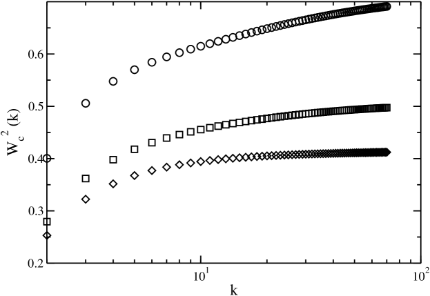
Figure 5: Log-linear plot of $W_{c}^{2}(k)$ as a function of $k$ for $\lambda=\ 2.5$, $r=-0.255$ ($\circ$), $-7.10^{-03}$ ($\Box$) and $0.335$ ($r_{min}$) ($\diamond$). We can see that for $k>k^{*}$, where $k^{*}\approx 10$ the asymptotic behavior of $W_{c}^{2}(k)$ goes as $\ln k$ for $r<r_{min}$ and $r>r_{min}$ and goes as a const. for $r\simeq r_{min}$.

References

- (1) R. Pastor-Satorras and A. Vespignani, Phys. Rev. Lett. 86, 3200(2001).
- (2) E. López et al., Phys. Rev. Lett. 94, 248701 (2005); A. Barrat, M. Barthélemy, R. Pastor-Satorras and A. Vespignani, PNAS 101, 3747 (2004).
- (3) Z. Wu, et al., Phys. Rev. E. 71, 045101(R) (2005).
- (4) A. E. Motter, Phys. Rev. Lett 93, 098701 (2004).
- (5) J. Jost and M. P. Joy, Phys. Rev. E 65, 016201 (2001); X. F. Wang, Int. J. Bifurcation Chaos Appl. Sci. Eng. 12, 885 (2002); M. Barahona and L. M. Pecora, Phys. Rev. Lett. 89, 054101 (2002); S. Jalan and R. E. Amritkar, Phys. Rev. Lett. 90, 014101 (2003); T. Nishikawa et al., Phys. Rev. Lett. 91, 014101 (2003); A. E. Motter et al., Europhys. Lett. 69, 334 (2005); A. E. Motter et al., Phys. Rev. E 71, 016116 (2005).
- (6) G. Korniss, Phys. Rev. E 75, 051121 (2007).
- (7) R. Albert and A.-L. Barabási, Rev. Mod. Phys. 74, 47 (2002); S. Boccaletti, V. Latora, Y. Moreno, M. Chavez and D.-U. Hwang, Physics Report 424, 175 (2006).
- (8) A. Nagurney, J. Cruz, J. Dong, and D. Zhang, Eur. J. Oper. Res. 164, 120 (2005).
- (9) J. W. Scannell et al., Cereb. Cortex 9, 277 (1999).
- (10) S. Eubank, H. Guclu, V. S. A. Kumar, M. Marathe, A. Srinivasan, Z. Toroczkai and N. Wang, Nature 429, 180 (2004); M. Kuperman and G. Abramson, Phys Rev Lett 86, 2909 (2001).
- (11) A. L. Pastore y Piontti, P. A. Macri and L. A. Braunstein, Phys. Rev. E 76, 046117 (2007).
- (12) M. E. J. Newman, Phys. Rev. E 67, 026126 (2003).
- (13) Jae Dong Noh, Phys. Rev. E 76, 026116 (2007).
- (14) A. L. Pastore y Piontti, L. A. Braunstein and P. A. Macri, Physics Letters A 374, 4658-4663 (2010).
- (15) M. di Bernardo, F. Garofalo and F. Sorrentino, Proceeding of the 44th IEEE Conference on Decision and Control, and the European Control Conference 2005, Seville, Spain, December 12-15, 2005 (4616-4621); arXiv:cond-mat/0506236v3.
- (16) F. Family, J. Phys. A 19, L441 (1986).
- (17) S. F. Edwards and D. R. Wilkinson, Proc. R. Soc. London, Ser. A 381, 17 (1982).
- (18) M. Molloy and B. Reed, Random Struct. Algorithms 6, 161 (1995); Combinatorics, Probab. Comput. 7, 295 (1998).
- (19) S. Maslov and K. Sneppen, Science 296, 910 (2002); R. Xulvi-Bruner and I. M. Sokolov, Phys. Rev. E 70, 066102 (2004); R. Xulvi-Bruner and I. M. Sokolov, Acta Physica Polonica B 36, 1431 (2005).
- (20) M. E. J. Newman, Phys. Rev. Let. 103, 058701 (2009); J. C. Miller, Phys. Rev. E 80, 020901 (2009).
- (21) R. Cohen, S. Havlin, and D. ben-Avraham 446. Chap. 4 in ”Handbook of graphs and networks”, Eds. S. Bornholdt and H. G. Schuster, (Wiley-VCH, 2002).