Conservative model for synchronization problems in complex networks.

Abstract

In this paper we study the scaling behavior of the interface fluctuations (roughness) for a discrete model with conservative noise on complex networks. Conservative noise is a noise which has no external flux of deposition on the surface and the whole process is due to the diffusion. It was found that in Euclidean lattices the roughness of the steady state $W_{s}$ does not depend on the system size. Here, we find that for Scale-Free networks of $N$ nodes, characterized by a degree distribution $P(k)\sim k^{-\lambda}$, $W_{s}$ is independent of $N$ for any $\lambda$. This behavior is very different than the one found by Pastore y Piontti et. al [Phys. Rev. E 76, 046117 (2007)] for a discrete model with non-conservative noise, that implies an external flux, where $W_{s}\sim\ln N$ for $\lambda<3$, and was explained by non-linear terms in the analytical evolution equation for the interface [La Rocca et. al, Phys. Rev. E 77, 046120 (2008)]. In this work we show that in this processes with conservative noise the non-linear terms are not relevant to describe the scaling behavior of $W_{s}$.

I Introduction

It is known that many physical and dynamical processes employ complex networks as the underlying a substrate. For this reason many studies on complex networks are focused not only in their topology but also in the dynamic processes that run over them. Some examples of these kind of dynamical processes on complex networks are cascading failures Motter_prl , traffic flow Lopez_transport ; zhenhua , epidemic spreadings Pastorras_PRL_2001 and synchronization Jost-prl ; Korniss07 . In particular, synchronization problems are very important in the dynamics and fluctuations in task completion landscapes in causally constrained queuing networks Kozma05 , in supply-chain networks based on electronic transactions Nagurney , brain networks JWScanell , and networks of coupled populations in the synchronization of epidemic outbreaks eubank_2004 . For example, in the problem of the load balance on parallel processors the load is distributed between the processors. If the system is not synchronized, few processors have low load and they will have to wait for the most loaded processors to finish the task. The nodes (processors) of the system have to synchronize with their neighbors to ensure causality on the dynamics. The computational time will be given by the most loaded processors, thus synchronizing the system is equivalent to reduce or optimize the computational time. Synchronization problems deal with the optimization of the fluctuations of some scalar field $h$ (load in processing) in the system that will be optimal synchronized minimizing those fluctuations. To analyze synchronization problems is customary to study the height fluctuations of a non-equilibrium surface growth. If the scalar field on the nodes represents the interface height at each node, its fluctuations are characterized by the average roughness $W(t)$ of the interface at time $t$, given by $W\equiv W(t)=\left\{1/N\sum_{i=1}^{N}(h_{i}-\langle h\rangle)^{2}\right\}^{1/2},$ where $h_{i}\equiv h_{i}(t)$ is the height of node $i$ at time $t$, $\langle h\rangle$ is the mean value on the network, $N$ is the system size, and $\{.\}$ denotes an average over configurations. Pastore y Piontti et. al anita studied this mapping in Scale-Free (SF) networks Barabasi_sf of broadness $\lambda$ and size $N$ using a surface relaxation growth model (SRM) family with non-conservative noise and found that for $\lambda<3$ the saturation roughness $W_{s}$ scales as $W_{s}\sim\ln N$. Later, the evolution equation for the interface in this model was derived analytically crispre for any complex networks. The derived evolution equation has non-linear terms as a consequence of the heterogeneity of the network that together with the non-conservative noise are necessary to explain the $W_{s}\sim\ln N$ behavior for $\lambda<3$. However, there exist many physical processes where the noise is conservative and cannot be modeled as a flux deposition on a surface. In models without external flux, where particles are moved by diffusion, the total volume of the system remains unchanged. Examples of this kind of process are thermal fluctuations, diffusion by an external agent such as an electric field, load balance of parallel processors where the total load in the system is constant over a certain time interval. For the last example, the only flux is due to diffusion of the load from a processor to another. Though not extensively, conservative noise has already been studied in Euclidean lattices cneucli1 ; cneucli2 and it was found that $W_{s}$ does not depend on the system size $L$. The evolution equation of this process in Euclidean lattices can be well represented by an Edwards-Wilkinson (EW) process EW with conservative noise. In this paper we study this model in SF networks by simulations of the discrete model (Section II) and derive analytically its evolution equation for any complex networks (Section III). Those networks represents better the heterogeneity in the contacts in real systems, like the Internet, the WWW, networks of routers, etc.. We applied the mean-field approximation to the evolution equation and show that the scaling behavior of $W_{s}$ with $N$ (Section IV) is only due to finite size effects. To our knowledge this class of model was never studied before in complex networks.

II Simulations of the discrete model

In this model, at each time step a node $i$ is chosen with probability $1/N$. If we denote by $v_{i}$ the nearest-neighbor nodes of $i$ , then (1) if $h_{i}<h_{j}$, $\forall j\in v_{i}$ $\Rightarrow$ the scalar fields remains unchanged, else (2) if $h_{j}<h_{n}$, $\forall n\not=j\in v_{i}$ $\Rightarrow h_{j}=h_{j}+1$ and $h_{i}=h_{i}-1$. In that way the total height of the interface is conserved and we have that the average height is constant. We measure the roughness $W$ for SF networks, characterized by a power law tail in the degree distribution $P(k)\sim k^{-\lambda}$, where $k_{max}\geq k\geq k_{min}$ is the degree of a node, $k_{max}$ is the maximum degree, $k_{min}$ is the minimum degree and $\lambda$ measures the broadness of the distribution Barabasi_sf . To build the SF network we use the Molloy Reed (MR) Molloy algorithm or configurational model.

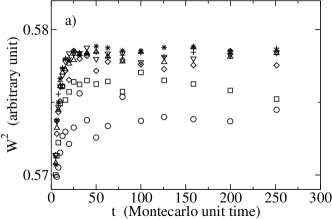
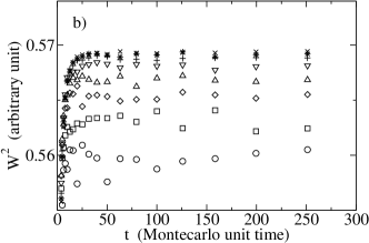
Figure 1: $W^{2}$ as a function of $t$ for the discrete model for a) $\lambda=\ 3.5$ for $N=64$ ($\circ$), $128$ ($\Box$), $256$ ($\diamond$), $512$ ($\bigtriangleup$), $1024$ ($\bigtriangledown$), $2048$ ($+$), $3072$ ($\star$) and $4096$ ($X$) and b) $\lambda=\ 2.5$ for $N=64$ ($\circ$), $128$ ($\Box$), $256$ ($\diamond$), $512$ ($\bigtriangleup$), $768$ ($\bigtriangledown$), $1024$ ($+$) and $1280$ ($\star$). Each curve was obtained with 10.000 realizations.

In Fig. 1 we plot $W^{2}$ as a function of the time $t$ for different system sizes and in Fig. 2 the steady state $W_{s}^{2}$ as a function of $N$, for (a) $\lambda=3.5$ and (b) $\lambda=2.5$. We can see that $W_{s}^{2}$ increases with $N$ but, as we will show later, this dependence in the system size is only due to finite size effects introduced by the correlated nature (dissortative) of the MR algorithm boguna . For all the results we use $k_{min}=2$ in order to ensure that the network is fully connected cohen , and assume that the initial configuration of $\{h_{i}\}$ is randomly distributed in the interval $[-0.5,0.5]$. Then, we have that $\langle h\rangle=0$.

III Derivation of the stochastic continuum equation

Next we derive the analytical evolution equation for the scalar field $h_{i}$ for every node $i$ in the conservative model in random graphs. The procedure chosen here is based on a coarse-grained (CG) version of the discrete Langevin equations obtained from a Kramers-Moyal expansion of the master equation VK ; Vveden ; lidia . The discrete Langevin equation for the evolution of the height in any growth model is given by Vveden ; lidia

$$\frac{\partial h_{i}}{\partial t}=\frac{1}{\tau}K^{1}_{i}+\eta_{i},$$ (1)

where $K^{1}_{i}$ takes into account the deterministic growth rules that produces the evolution of the scalar field $h_{i}$ on node $i$, $\tau=N\delta t$ is the mean time of attempts to change the scalar fields of the interface, and $\eta_{i}$ is a noise with zero mean and covariance given by Vveden ; lidia

$$\{\eta_{i}(t)\eta_{j}(t^{\prime})\}=\frac{1}{\tau}K_{ij}^{2}\delta(t-t^{\prime})\ .$$ (2)

More explicitly, $K^{1}_{i}$ and $K_{ij}^{2}$ are the two first moments of the transition rate and they are given by

$$K^{1}_{i}=\sum_{j=1}^{N}A_{ij}\left[P_{ij}-P_{ji}\right]\ ,$$ (3)

$$K_{ij}^{2}=\frac{1}{\tau}K^{1}_{i}\delta_{ij}-\frac{1}{\tau}\sum_{n=1}^{N}A_{in}(P_{in}+P_{ni})(\delta_{nj}-\delta_{ij})\ ,$$ (4)

where $\{A_{ij}\}$ is the adjacency matrix ($A_{ij}=1$ if $i$ and $j$ are connected and zero otherwise) and $P_{ij}$ is the rule that represents the growth contribution to node $i$ by relaxation from its neighbor $j$. In our model the network is undirected, then $A_{ij}=A_{ji}$. As the rules for this model are very complex if we allow degenerate scalar fields, we simplify the problem taking random initial conditions [See discrete rules on Sec.II]. Thus,

$$P_{ij}=\Theta(h_{j}-h_{i})\prod_{n\in v_{j}}[1-\Theta(h_{i}-h_{n})]\ ,$$

where $\Theta$ is the Heaviside function given by $\Theta(x)=1$ if $x\geq 0$ and zero otherwise, with $x=h_{t}-h_{s}\equiv\Delta h$. Without lost of generality, we take $\tau=1$.

In the CG version $\Delta h\rightarrow 0$; thus after expanding an analytical representation of $\Theta(x)$ in Taylor series around $x=0$ to first order in $x$, we obtain

$$K^{1}_{i} =\ c_{0}\ \sum_{j=1}^{N}A_{ij}\ \left[\Omega(k_{j})-\Omega(k_{i})\right]\ +\ c_{1}\ \sum_{j=1}^{N}A_{ij}\ \left[\Omega(k_{j})+\Omega(k_{i})\right]\ (h_{j}-h_{i})$$ (5)

$$+\ \frac{c_{1}c_{0}}{(1-c_{0})}\ \sum_{j=1}^{N}A_{ij}\Omega(k_{j})\ \left[\sum_{n=1,n\not=i}^{N}A_{jn}(h_{n}-h_{i})\right]+O((\Delta h)^{2})\ ,$$

where $c_{0}$ and $c_{1}$ are the first two coefficients of the expansion of $\Theta(x)$ and $\Omega(k_{i})=(1-c_{0})^{k_{i}-1}$ is the weight on the link $ij$ introduced by the dynamic process.

Notice that the network is undirected and the noise is conservative, thus the average noise correlation [see Eq. (2)] is $\langle\eta_{i}(t)\eta_{j}(t^{{}^{\prime}})\rangle=0$, where $\langle~{}~{}\rangle$ represents average over all the nodes of the network. Notice that in Eq. (5) the non-linear terms are disregarded. As we will show below, for this conservative noise model these terms are not necessary to explain the scaling behavior of $W_{s}$ with $N$.

We numerically integrate our evolution equation Eq. (1) in SF networks using the Euler method with a representation of the Heaviside function given by $\Theta(x)=(1+\tanh[U(x+z)])/2$, where $U$ is the width and $z=1/2$ lidia . With this representation, $c_{0}=(1+\tanh[U/2])/2$ and $c_{1}=(1-\tanh^{2}[U/2])\ U/2$. We assume that the initial configuration of $\{h_{i}\}$ is randomly distributed in the interval $[-0.5,0.5]$ and for the conservative noise we used the algorithm described in ruidoconser : at each time step, for every node in the network and for any of its nearest neighbor we add a random number in the interval [-0.5,0.5] and remove this amount to one of the nearest neighbor nodes.

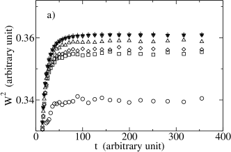
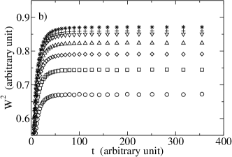
Figure 3: $W^{2}$ as a function of $t$ from the integration of the evolution equation: a) $\lambda=\ 3.5$ for $N=64$ ($\circ$), $128$ ($\Box$), $256$ ($\diamond$), $512$ ($\bigtriangleup$), $1024$ ($\bigtriangledown$), $1536$ ($+$) and $2048$ ($\star$) and b) $\lambda=\ 2.5$ for $N=64$ ($\circ$), $128$ ($\Box$), $256$ ($\diamond$), $512$ ($\bigtriangleup$), $768$ ($\bigtriangledown$), $1024$ ($+$) and $1280$ ($\star$). For all the integrations we use $U=0.5$ and typically $1.000$ realizations of networks.

In Fig. 3 we plot $W^{2}$ as a function of $t$ from the integration of Eq. (1) for (a) $\lambda=3.5$ and (b) $\lambda=2.5$, and different values of $N$ with $k_{min}=2$. For the time step integration we chose $\Delta t\ll 1/k_{max}$ according to Ref pasointeg . In Fig. 4 we plot the steady state $W_{s}^{2}$ as a function of $N$ for (a) $\lambda=3.5$ and (b) $\lambda=2.5$. We can see that $W_{s}^{2}$ depends weakly on $N$, but as shown below this size dependence is due to finite size effects introduced by the MR construction. Next we derive the mean field approximation in order to explain the nature of the corrections to the scaling.

IV Mean field approximation for the evolution equation

We apply a mean field (MF) approximation to the linear terms of Eq. (5). In this approximation we consider $1\ll k_{min}\ll k_{max}$. Taking $C_{ij}=A_{ij}\Omega(k_{j})$ and $T_{ijn}=A_{ij}A_{jn}\Omega(k_{j})$, then

$$K^{1}_{i} =\ c_{0}\ \left[C_{i}-k_{i}\Omega(k_{i})\right]\ +\ c_{1}C_{i}\left[\sum_{j=1}^{N}\frac{C_{ij}h_{j}}{C_{i}}-h_{i}\right]$$

$$+\ c_{1}\Omega(k_{i})k_{i}\left[\sum_{j=1}^{N}\frac{A_{ij}h_{j}}{k_{i}}-h_{i}\right]$$

$$+\ \frac{c_{1}c_{0}}{(1-c_{0})}\ T_{i}\left[\sum_{j=1}^{N}\sum_{n=1,n\not=i}^{N}\frac{T_{ijn}h_{n}}{T_{i}}-h_{i}\right]\ ,$$

where

$$C_{i}= \sum_{j=1}^{N}C_{ij}\ ;$$

$$T_{i}= \sum_{j=1}^{N}\sum_{n=1,n\not=i}^{N}T_{ijn}\ .$$ (7)

Disregarding the fluctuations, we take $\sum_{j=1}^{N}A_{ij}h_{j}/k_{i}\approx\langle h\rangle$, $\sum_{j=1}^{N}C_{ij}h_{j}/C_{i}\approx\langle h\rangle$, and $\sum_{j=1}^{N}\sum_{n=1,n\not=i}^{N}T_{ijn}h_{n}/T_{i}\approx\langle h\rangle$. From Eq. (IV), we can approximate $C_{i}$ by $C_{i}(k_{i})\approx k_{i}\int_{k_{min}}^{k_{max}}P(k|k_{i})\ \Omega(k)\ dk$ Korniss07 , where $P(k|k_{i})$ is the conditional probability that a node with degree $k_{i}$ is connected to another with degree $k$. For uncorrelated networks $P(k|k_{i})=kP(k)/\langle k\rangle$ Barabasi_sf , then $C_{i}(k_{i})\approx I_{1}\ k_{i}/\langle k\rangle$ with $I_{1}=\int_{k_{min}}^{k_{max}}P(k)\ k\ \Omega(k)\ dk$ . Making the same assumption for $T_{i}$, we obtain $T_{i}(k_{i})\approx I_{2}\ k_{i}/\langle k\rangle$ with $I_{2}=\int_{k_{min}}^{k_{max}}P(k)\ k\ (k-1)\ \Omega(k)\ dk$. Then, the linearized evolution equation for the heights in the MF approximation can be written as

$$\frac{\partial{h_{i}}}{\partial t} = F_{i}(k_{i})+\nu_{i}(k_{i})\ (\langle h\rangle-h_{i})+\eta_{i}\ ,$$ (8)

where $F_{i}(k_{i})=c_{0}k_{i}\left[I_{1}/\langle k\rangle-\Omega(k_{i})\right]$ represents a local driving force, $\nu_{i}(k_{i})=c_{1}k_{i}(b+\Omega(k_{i}))$ is a local superficial tension-like coefficient with $b=[I_{1}+I_{2}c_{0}/(1-c_{0})]/\langle k\rangle$. This mean field approximation reveals the network topology dependence through $P(k)$.

Taking the average over the network in Eq. (8), $\partial\langle h\rangle/\partial t=1/N\sum_{i=1}^{N}F_{i}=0$, then $\langle h\rangle$ is constant in time. The solution of Eq. (8) VK is given by

$$h_{i}(t) = \int_{0}^{t}e^{-\nu_{i}(t-s)}\ (F_{i}+\nu_{i}\langle h\rangle+\eta_{i}(s))\ ds$$ (9)

$$= \frac{F_{i}+\nu_{i}\langle h\rangle}{\nu_{i}}(1-e^{-\nu_{i}t})+\int_{0}^{t}e^{-\nu_{i}(t-s)}\eta_{i}(s)\ ds\ .$$

Using Eq. (9) and the fact that in our model with the initial conditions we use $\langle h\rangle=0$, we find the two-point correlation function

$$\left\{h_{i}(t_{1})h_{j}(t_{2})\right\} =\ \left(\frac{F_{i}}{\nu_{i}}\right)\left(\frac{F_{j}}{\nu_{j}}\right)(1-e^{-\nu_{i}t})(1-e^{-\nu_{j}t})$$

$$+ \int_{0}^{t_{2}}\int_{0}^{t_{1}}e^{-\nu_{i}(t_{1}-s_{1})}e^{-\nu_{j}(t_{2}-s_{2})}\left\{\eta_{i}(s_{1})\eta_{j}(s_{2})\right\}\ ds_{1}ds_{2}\ .$$

For $t>max\left\{1/\nu_{i}\right\}$, we can write $W_{s}$ as

$$W_{s}^{2}=\{<h_{i}^{2}>\}=\frac{1}{N}\sum_{i=1}^{N}\left(\frac{F_{i}}{\nu_{i}}\right)^{2}+\frac{1}{N}\sum_{i=1}^{N}\frac{K_{ii}^{2}}{\nu_{i}}\ ,$$ (10)

where $K_{ii}^{2}$ [See Eq. (4)] is given by

$$K_{ii}^{2}=\sum_{j=1}^{N}A_{ij}\left[P_{ij}+P_{ji}\right]\approx c_{0}k_{i}\ \left[\frac{I_{1}}{\langle k\rangle}+\Omega(k_{i})\right]\ .$$

For SF networks it can be shown that $I_{1},I_{2}\sim\mbox{const.}+k_{max}\exp(-k_{max}\mbox{const.})$, where $k_{max}\sim N^{1/(\lambda-1)}$ for MR networks; thus we can considerer the quantities $I_{1}$ and $I_{2}$ as independent of $N$.

From Eq. (10) and using the expressions for $F_{i}$, $\nu_{i}$ and $K_{ii}^{2}$, we have

$$W_{s}^{2}=\left(\frac{c_{0}}{c_{1}}\right)^{2}B^{2}\frac{1}{N}\sum_{i=1}^{N}\left(f_{-}(k_{i})\right)^{2}+\frac{c_{0}}{c_{1}}B\frac{1}{N}\sum_{i=1}^{N}f_{+}(k_{i})\ ,$$ (11)

where

$$f_{\pm}(k_{i})=\frac{1\pm\frac{\langle k\rangle}{I_{1}}\ \Omega(k_{i})}{1+\frac{\langle k\rangle}{I_{2}}\frac{c_{0}}{1-c_{0}}\ \Omega(k_{i})}\ ,$$

and $B=1/(1+c_{0}I_{2}/(1-c_{0})I_{1})$. Taking the continuum limit we find another expression for Eq. (11) as

$$W_{s}^{2}=\left(\frac{c_{0}}{c_{1}}\right)^{2}B^{2}\int_{k_{min}}^{k_{max}}p(k)(f_{-}(k))^{2}\ dk+\frac{c_{0}}{c_{1}}B\int_{k_{min}}^{k_{max}}p(k)f_{+}(k)\ dk\ .$$

The function $f_{\pm}(k)$ has a crossover at $k=k^{*}$ , where $k^{*}$ is the crossover degree between the two different behaviors, then

1) for $k<k^{*}\Rightarrow f_{\pm}(k)\approx\pm\ \langle k\rangle\ \Omega(k)/I_{1}/2$, and

2) for $k>k^{*}\Rightarrow f_{\pm}(k)\approx 1$.

As $k^{*}$ is the crossover between two different behaviors of $f_{\pm}(k)$, and the numerator of the function diverges faster than the denominator, we have $1\approx\langle k\rangle\ \Omega(k^{*})/I_{1}$ thus $k^{*}\approx\ln(I_{1}/\langle k\rangle)/\ln(1-c_{0})$. Then,

$$W_{s}^{2} =\left[\left(\frac{c_{0}}{c_{1}}\right)^{2}B^{2}+\frac{c_{0}}{c_{1}}B\right]\int_{k^{*}}^{k_{max}}p(k)dk+\left(\frac{c_{0}B}{2c_{1}I_{1}}\right)^{2}\langle k\rangle^{2}\int_{k_{min}}^{k^{*}}p(k)(\Omega(k))^{2}dk$$

$$+\left(\frac{c_{0}B}{2c_{1}I_{1}}\right)\langle k\rangle\int_{k_{min}}^{k^{*}}p(k)\Omega(k)dk\ .$$

Even thought $k^{*}$ depends on $k_{max}$, it can be demonstrated that the two last integrals depends weakly on $N$ and can be considerer as constant. Then, introducing the corrections due to finite size effects trough $k_{max}$ in $\langle k\rangle$, we obtain

$$W_{s}^{2}\sim W_{s}^{2}(\infty)\left(1+\frac{A_{1}}{N}+\frac{A_{2}}{N^{\frac{\lambda-2}{\lambda-1}}}+\frac{A_{3}}{N^{2\frac{\lambda-2}{\lambda-1}}}\right)\ .$$ (12)

where $A_{1}$, $A_{2}$ and $A_{3}$ do not depend on $k_{max}$.

In Fig. 2 and Fig. 4 the dashed lines represent the fitting of the curves with Eq. (12) considering finite-size effects introduced by the MR construction. We can see that this equation represents very well the finite size effects of this model. This means that even though the networks is heterogeneous, the non-linear terms are not necessary to explain the $N$ independence of $W_{s}$ when a conservative noise is used. Notice that even when our network is correlated in the degree, the expression for $W_{s}^{2}$ found describe very well the scaling behavior with $N$ as shown in the insets of Fig. 2 and 4. This model suggest a useful load balance algorithm suitable for processors synchronization in parallel computation. Our results show that the algorithm could be useful when one want to increase the number of processors and its general behavior is well represented by a simple mean field equation.

V Summary

In summary, in this paper we study a conservative model in SF networks and find that the roughness of the steady state is a constant and its dependence on $N$ for any $\lambda$ it is only due to finite size effects. We derive analytically the evolution equation for the model, and retain only linear terms because they are enough to explain the scaling behavior of $W_{s}$. Finally, we apply the mean field approximation to the equation and we calculate explicitly the corrections to scaling of $W_{s}$. This approximation describe very well the behavior of the model and shows clearly that the corrections are due to finite size effects.

VI Acknowledgments

This work has been supported by UNMdP and FONCyT (Pict 2005/32353).

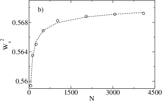
Figure 2: $W_{s}^{2}$ as a function of $N$ for a) $\lambda=\ 3.5$ and b) $\lambda=\ 2.5$ in symbols for the same system sizes of the Fig 1. The dashed lines represent the fitting with Eq. (12), obtained in the MF approximation by considering the finite-size effects introduced by the MR construction.

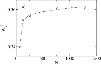
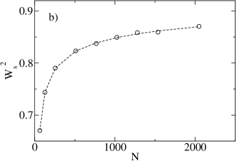
Figure 4: $W_{s}^{2}$ as a function of $N$ for a) $\lambda=\ 3.5$ and b) $\lambda=\ 2.5$ in symbols for the same system sizes of the Fig 3. The dashed lines represent the fitting with Eq. (12), obtained by considering the finite-size effects introduced by the MR construction.

References

• (1) A. E. Motter, Phys. Rev. Lett 93, 098701 (2004).
• (2) E. López et al., Phys. Rev. Lett. 94, 248701 (2005); A. Barrat, M. Barthélemy, R. Pastor-Satorras and A. Vespignani, PNAS 101, 3747 (2004).
• (3) Z. Wu, et al., Phys. Rev. E. 71, 045101(R) (2005).
• (4) R. Pastor-Satorras and A. Vespignani, Phys. Rev. Lett. 86, 3200(2001).
• (5) J. Jost and M. P. Joy, Phys. Rev. E 65, 016201 (2002); X. F. Wang, Int. J. Bifurcation Chaos Appl. Sci. Eng. 12, 885 (2002); M. Barahona and L. M. Pecora, Phys. Rev. Lett. 89, 054101 (2002); S. Jalan and R. E. Amritkar, Phys. Rev. Lett. 90, 014101 (2003); T. Nishikawa et al., Phys. Rev. Lett. 91, 014101 (2003); A. E. Motter et al., Europhys. Lett. 69, 334 (2005); A. E. Motter et al., Phys. Rev. E 71, 016116 (2005).
• (6) G. Korniss, Phys. Rev. E 75, 051121 (2007).
• (7) H. Guclu, G. Korniss and Z. Toroczkai, Chaos 17, 026104 (2007).
• (8) A. Nagurney, J. Cruz, J. Dong, and D. Zhang, Eur. J. Oper. Res. 164, 120 (2005).
• (9) J. W. Scannell et al., Cereb. Cortex 9, 277 (1999).
• (10) S. Eubank, H. Guclu, V. S. A. Kumar, M. Marathe, A. Srinivasan, Z. Toroczkai and N. Wang, Nature 429, 180 (2004); M. Kuperman and G. Abramson, Phys Rev Lett 86, 2909 (2001).
• (11) A. L. Pastore y Piontti, P. A. Macri and L. A. Braunstein, Phys. Rev. E 76, 046117 (2007).
• (12) R. Albert and A.-L. Barabási, Rev. Mod. Phys. 74, 47 (2002); S. Boccaletti, V. Latora, Y. Moreno, M. Chavez and D.-U. Hwang, Physics Report 424, 175 (2006).
• (13) F. Family, J Phys. A 19, L441 (1986).
• (14) C. E. La Rocca, L. A. Braunstein and P. A. Macri, Phys. Rev. E 77, 046120 (2008).
• (15) Youngkyun Jung and In-mook Kim, Phys. Rev. E 59, 7224 (1999).
• (16) In-mook Kim, Jin Yang and Youngkyun Jung, Journal of the Korean Physical Society 34, 314 (1999).
• (17) S. F. Edwards and D. R. Wilkinson, Proc. R. Soc. London, Ser. A 381, 17 (1982).
• (18) M. Molloy and B. Reed, Random Struct. Algorithms 6, 161 (1995); Combinatorics, Probab. Comput. 7, 295 (1998).
• (19) M. Boguñá, R. Pastor-Satorras, and A. Vespignani, Eur. Phys. J. B 38, 205 (2004).
• (20) R. Cohen, S. Havlin, and D. ben-Avraham 446. Chap. 4 in ”Handbook of graphs and networks”, Eds. S. Bornholdt and H. G. Schuster, (Wiley-VCH, 2002).
• (21) N. G. Van Kampen, Stochastic Processes in Physics and Chemistry, North-Holland, Amsterdam (1981).
• (22) D. D. Vvedensky, Phys. Rev. E 67, 025102(R) (2003).
• (23) L. A. Braunstein, R. C. Buceta, C. D. Archubi and G. Costanza, Phys. Rev. E 62, 3920 (2000).
• (24) A. Ballestad, B. J. Ruck, J. H. Schmid, M. Adamcyk, E. Nodwell, C. Nicoll, and T. Tiedje, Phys. Rev. B 65, 205302 (2004).
• (25) B. Kozma, M. B. Hastings and G. Korniss, J. Stat. Mech. Theor. Exp. (2007) P08014.
Refer to caption
Refer to caption