A mechanism to synchronize fluctuations in scale free networks using growth models.

Abstract

In this paper we study the steady state of the fluctuations of the surface for a model of surface growth with relaxation to any of its lower nearest neighbors (SRAM) [F. Family, J. Phys. A 19, L441 (1986)] in scale free networks. It is known that for Euclidean lattices this model belongs to the same universality class as the model of surface relaxation to the minimum (SRM). For the SRM model, it was found that for scale free networks with broadness $\lambda$, the steady state of the fluctuations scales with the system size $N$ as a constant for $\lambda\geq 3$ and has a logarithmic divergence for $\lambda<3$ [Pastore y Piontti et al., Phys. Rev. E 76, 046117 (2007)]. It was also shown [La Rocca et al., Phys. Rev. E 77, 046120 (2008)] that this logarithmic divergence is due to non-linear terms that arises from the topology of the network. In this paper we show that the fluctuations for the SRAM model scale as in the SRM model. We also derive analytically the evolution equation for this model for any kind of complex graphs and find that, as in the SRM model, non-linear terms appear due to the heterogeneity and the lack of symmetry of the network. In spite of that, the two models have the same scaling, but the SRM model is more efficient to synchronize systems.

, , , .

Recently, much effort has been devoted to the study of dynamics in complex networks. This is because many physical and dynamic processes use complex networks as substrates to propagate, such as epidemic spreading [1], traffic flow [2, 3, 4] and synchronization [5, 6]. In particular, synchronization problems in networks are very important in many fields such as the brain network [7], networks of coupled populations in epidemic outbreaks [8] and the dynamics and fluctuations of task completion landscapes in causally-constrained queuing networks [9]. Synchronization deals with the optimization of the fluctuations in the steady state of some scalar field $h$, that can represent the neuronal population activity in brain networks, infected population in epidemics and jobs or packets in queuing networks. It is particularity interesting to understand how to reduce the load excess in communication networks in the steady state. This problem can be mapped into a problem of non-equilibrium surface growth where $h$ is a random scalar field on the nodes that could represent the total flow on the network and the load excess could represent the overload of flow that a node should handle. Then, a way to reduce the load excess is to reduce the fluctuations of that scalar field. Recently, Pastore y Piontti et. al [10] used the model of surface relaxation to the minimum (SRM), that allow balancing the load, reducing the fluctuations in scale free (SF) networks with degree distribution given by $P(k)\sim k^{-\lambda}$, ($k\geq k_{min}$) with $k$ the degree of a node, $k_{min}$ the minimum degree that a node can have, and $\lambda$ the broadness of the distribution [11]. Given a scalar field $h$ on the nodes, that in surface problems represents the interface height at each node, the fluctuations are characterized by the average roughness $W(t)$ of the interface at time $t$, given by $W\equiv W(t)=\left\{1/N\sum_{i=1}^{N}(h_{i}-\langle h\rangle)^{2}\right\}^{1/2},$ where $h_{i}\equiv h_{i}(t)$ is the height of the node $i$ at time $t$, $\langle h\rangle=(1/N)\sum_{i=1}^{N}h_{i}$, $N$ is the system size, and $\{.\}$ denotes average over configurations.

The aim of this paper is to study the steady state of $W\equiv W_{s}$ for the model of surface growth with relaxation to any of its lower nearest neighbors (SRAM) [12]. We find that this model has the same behavior with the system size as the SRM model for every $\lambda$, even though the SRM model is more efficient to reduce the fluctuations and to enhance synchronization than the SRAM model, as we show later. Moreover, we derive analytically the general evolution equation for the SRAM model for any kind of random graph.

1 Surface relaxation models

In the SRM model, at each time step a node $i$ is chosen with probability $1/N$. If we denote by $v_{i}$ the nearest-neighbor nodes of $i$, then

$$\mbox{if}\left\{\begin{array}[]{ll}(1)\ h_{i}\leq h_{j},\ \forall j\in v_{i}&\Rightarrow h_{i}=h_{i}+1\\ (2)\ h_{j}<h_{n}\ \forall n\not=j\in v_{i}&\Rightarrow h_{j}=h_{j}+1.\end{array}\right.$$

The SRAM model has the same rule (1) as the SRM model, but the second rule is different: the chosen node can relax to any of its lower $m$ neighbors with probability $1/m$. Then, the rules for the SRAM model are

$$\mbox{if}\ \left\{\begin{array}[]{ll}(1)\ h_{i}\leq h_{j},\ \forall j\in v_{i}&\Rightarrow h_{i}=h_{i}+1,\mbox{else}\\ (2)\ \exists\ m\ \mbox{nodes}\ j\in v_{i}\ \mbox{with}\ h_{j}<h_{i}&\Rightarrow h_{j}=h_{j}+1\ \mbox{with probability}\ 1/m.\end{array}\right.$$ (3)

It is known that in Euclidean lattices of typical linear size $L$ the SRM and the SRAM models belong to the same universality class [12, 13], with

$$W(t)\sim\cases{\begin{array}[]{rl}t^{\beta},&t<t_{s}\ ,\\ L^{\alpha},&t>t_{s}\ ,\end{array}}$$

where $t_{s}$ is the saturation time which scales as $t_{s}\sim L^{z}$. Here, the exponent $\beta$ is the growth exponent, $\alpha$ is the roughness exponent and $z$ is the dynamical exponent that characterizes the growth correlations given by $z=\alpha/\beta$. For $1$ dimension, these exponents are $\beta=1/4$, $\alpha=1/2$ and $z=2$. Moreover, both growth models belong to the same universality class as the Edward-Wilkinson (EW) equation,

$$\frac{\partial h(x,t)}{\partial t}=\nu\nabla^{2}h(x,t)+\eta(x,t)\ ,$$

where $\nu$ is the coefficient of surface tension and $\eta(x)$ is a Gaussian noise with zero mean and covariance given by

$$\{\eta(x,t)\eta(x^{{}^{\prime}},t^{{}^{\prime}})\}=2D\delta(x-x^{{}^{\prime}})\delta(t-t^{{}^{\prime}})\ .$$

Here, $D$ is the diffusion coefficient and is taken as a constant. The fact that these models are represented by the same phenomenological equation is due to the symmetry of those models on the underlying Euclidean substrate [14]. The extension of the EW equation to any unweighted graph with $N$ nodes is described by

$$\frac{\partial h_{i}(t)}{\partial t}=\nu\sum_{j=1}^{N}A_{ij}(h_{j}(t)-h_{i}(t))+\eta_{i}(t)\ ,$$ (4)

where $i$ and $j$ are nodes of the graph, $\{A_{ij}\}$ is the adjacency matrix ($A_{ij}=1$ if $i$ and $j$ are connected and zero otherwise), $\nu$ represents the same as in Euclidean lattices and $\eta_{i}(t)$ is a white Gaussian noise with zero mean and covariance given by

$$\{\eta_{i}(t)\eta_{j}(t^{{}^{\prime}})\}=2D\ \delta_{ij}\delta(t-t^{{}^{\prime}})\ ,$$

being $D$ the same as in Euclidean lattices.

In Ref. [10] it was found that the saturation regime of $W_{s}$ in SF networks scales with $N$ as

$$W_{s}\sim\cases{\begin{array}[]{ll}const.&\mbox{for}\ \lambda\geq 3,\\ \ln N&\mbox{for}\ 2<\lambda<3\ .\end{array}}.$$ (5)

It was also shown that the EW equation given by Eq. (4) predicts that in the thermodynamic limit $W_{s}\sim 1/\langle k\rangle$ for any random graph [6]. Then, the unweighted EW equation in random graphs cannot describe the SRM model. La Rocca et. al [15], using a temporal continuous approach, derived the evolution equation that describes the SRM model. They found that the logarithmic divergence for $\lambda<3$ cannot be explained by the unweighted EW equation [See Eq. (4)] in graphs. The equation derived in Ref [15] contains non-linear terms and weights that appear as a consequence of the heterogeneous topology that a SF has for $\lambda<3$, even though the network is unweighted. The heterogeneity breaks the symmetry $h\to-h$ of Eq. (4). For $\lambda\geq 3$ the heterogeneity is not strong enough and the non-linear terms are negligible for the system sizes studied there, and the behavior of the fluctuations becomes well described by a weighted EW equation. It is not unexpected that transport processes in random heterogeneous graphs behave differently than in Euclidean lattices due to the fact that the nodes with high degrees (hubs) play a mayor role in transport. For example, reaction-diffusion processes behave very differently in homogeneous lattices than in SF networks with $2<\lambda<3$ due to the presence of hubs which control the behavior for long times [16, 17]. The hubs are responsible of a superdiffusive regime because they diminish the distances.

2 Saturation results for the SRAM model

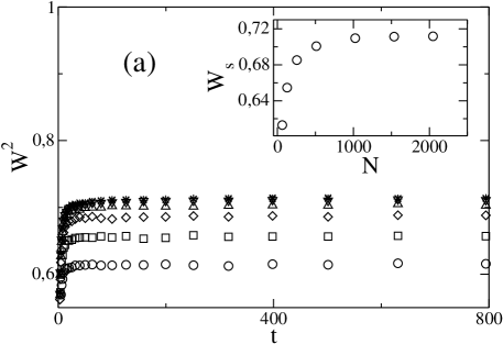
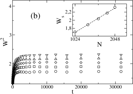
Figure 1: $W^{2}$ as a function of $t$ for the SRAM model: $(a)\ \lambda=3.5$ for $N=64$ ($\bigcirc$), $128$ ($\Box$), $256$ ($\diamond$), $512$ ($\bigtriangleup$), $1024$ ($\bigtriangledown$), $1536$ ($\star$) and $2048$ ($X$). $(b)\ \lambda=2.5$ for $N=1024$ ($\bigcirc$), $1280$ ($\Box$), $1536$ ($\diamond$), $1792$ ($\bigtriangleup$), and $2048$ ($\bigtriangledown$). In the inset figures we plot $W_{s}$ as a function of $N$ in symbols. The inset figure of $(b)$ is in log-linear scale and the dashed line represents the logarithmic fitting of $W_{s}$ with $N$.

We construct our networks using the Molloy-Reed (MR) algorithm [18], with $k_{min}=3$ in order to ensure that the network is fully connected. The initial conditions for the scalar field $\{h\}$ were drawn from a random uniform distribution between $[0,1]$. In Fig. 1, we plot $W^{2}$ as a function of $t$ for $\lambda=3.5$ and $2.5$ and different values of $N$. In the insets of Fig. 1 we plot $W_{s}$ as a function of $N$. We can see that for $\lambda=3.5$, $W_{s}$ increases, but asymptotically goes to a constant and all the $N$ dependence is due to finite-size effects as in the SRM model [10]. However, for $\lambda=2.5$ we find that $W_{s}\sim\ln N$, as in the SRM model. This is shown in the inset of Fig. 1$(b)$ in log-linear scale. Then, $W_{s}$ for both models scales in the same way for SF networks, with a logarithmic divergence for $\lambda<3$ and as a constant for $\lambda\geq 3$.

3 Analytical Evolution Equation

Next, we derive analytically the evolution equation for $\{h\}$ of the SRAM model for any kind of random graphs.

The procedure chosen here is the same as the one used in Ref. [15] and is based on a coarse-grained (CG) version of the discrete Langevin equations obtained from a Kramers-Moyal expansion of the master equation [19, 13, 20]. The discrete Langevin equation for the evolution of the height in any growth model is given by [13, 20]

$$\frac{\partial h_{i}}{\partial t}=\frac{1}{\tau}G_{i}+\eta_{i}\ ,$$ (6)

where $G_{i}$ represents the deterministic growth rules that cause the evolution of the node $i$, $\tau=N\delta t$ is the mean time to grow a layer of the interface, and $\eta_{i}$ is a Gaussian noise with zero mean and covariance given by [13, 20]

$$\{\eta_{i}(t)\eta_{j}(t^{\prime})\}=\frac{1}{\tau}G_{i}\delta_{ij}\delta(t-t^{\prime})\ .$$ (7)

If $k_{\gamma}$ represents the degree of node $\gamma$, we can write $G_{i}$ more explicitly as

$$G_{i}=\omega_{i}+\sum_{j=1}^{N}A_{ij}\ (\omega_{j}^{1}+\omega_{j}^{2}+...+\omega_{j}^{k_{j}})\ ,$$ (8)

where $\omega_{i}$ is the growth contribution by deposition on the node $i$ and $\omega_{j}^{m}$ is the growth contribution to the node $i$ by relaxation from its neighbor $j$ with probability $1/m$, being $m$ the number of neighbors of the node $j$ with smaller heights than the node $j$. Then,

$$\omega_{i}=\prod_{j\in v_{i}}\left[1-\Theta(h_{i}-h_{j})\right],$$

$$\omega_{j}^{1}=\left[1-\Theta(h_{i}-h_{j})\right]\prod_{n\in v_{j},n\not=i}\left[1-\Theta(h_{j}-h_{n})\right]\ ,$$

$$\omega_{j}^{2}=\left[1-\Theta(h_{i}-h_{j})\right]\prod_{n\in v_{j},n\not=i,m}\left[1-\Theta(h_{j}-h_{n})\right]\frac{1}{2}\left[1-\Theta(h_{m}-h_{j})\right]\ ,$$

$$\omega_{j}^{3}=\left[1-\Theta(h_{i}-h_{j})\right]\prod_{n\in v_{j},n\not=i,m,\ell}\left[1-\Theta(h_{j}-h_{n})\right]\frac{1}{3}\left[1-\Theta(h_{m}-h_{j})\right]\left[1-\Theta(h_{\ell}-h_{j})\right]\ ,$$

.

.

.

$$\omega_{j}^{k_{j}}=\left[1-\Theta(h_{i}-h_{j})\right]\prod_{n\in v_{j},n\not=i}\left[1-\Theta(h_{n}-h_{j})\right]\frac{1}{k_{j}}\ .$$

Here, $\Theta$ is the Heaviside function given by $\Theta(x)=1$ if $x\geq 0$ and zero otherwise, with $x=h_{t}-h_{s}\equiv\Delta h$. Without loss of generality, we take $\tau=1$ and assume that the initial configuration of $\{h_{i}\}$ is random. A schematic plot of the growing rules are shown in Fig. 2 where the rule (1) represent $\omega_{i}$, (2) represent $\omega_{j}^{1}$ and (3) represent $\omega_{j}^{2}$.

In the CG version $x\rightarrow 0$; thus after expanding an analytical representation of $\Theta(x)$ in Taylor series around $x=0$ to second order in $x$, we obtain

$$G_{i} =\ a^{k_{i}}\ +\ \sum_{j=1}^{N}C_{ij}\ +\ c_{1}a^{k_{i}-1}\ \sum_{j=1}^{N}A_{ij}(h_{j}-h_{i})$$ (9)

$$+\ \frac{c_{1}}{a}\ \sum_{j=1}^{N}C_{ij}(h_{j}-h_{i})\ +\ \frac{c_{1}}{a}\ \sum_{j=1}^{N}T_{ij}\sum_{n=1,n\not=i}^{N}A_{jn}(h_{n}-h_{j})$$

$$-\ \frac{c_{2}}{a}\ \sum_{j=1}^{N}C_{ij}(h_{j}-h_{i})^{2}\ -\ a^{k_{i}-1}\left[c_{2}+\frac{c_{1}^{2}}{2a}\right]\sum_{j=1}^{N}A_{ij}(h_{j}-h_{i})^{2}$$

$$+\ \sum_{j=1}^{N}\left[\frac{c_{1}^{2}}{2a^{2}}Q_{ij}-\frac{c_{2}}{a}C_{ij}\right]\left[\sum_{n=1,n\not=i}^{N}A_{jn}(h_{n}-h_{j})^{2}\right]$$

$$+\ \frac{a^{k_{i}-2}c_{1}^{2}}{2}\left[\sum_{j=1}^{N}A_{ij}(h_{j}-h_{i})\right]^{2}\ +\ \frac{c_{1}^{2}}{a^{2}}\sum_{j=1}^{N}T_{ij}(h_{j}-h_{i})\left[\sum_{n=1,n\not=i}^{N}A_{jn}(h_{n}-h_{j})\right]$$

$$-\ \frac{c_{1}^{2}}{2a^{2}}\sum_{j=1}^{N}Q_{ij}\left[\sum_{n=1,n\not=i}^{N}A_{jn}(h_{n}-h_{j})\right]^{2}\ ,$$

where $a=(1-c_{0})$, $c_{0}$, $c_{1}$ and $c_{2}$ are the first three coefficients of the expansion of the $\Theta(x)$ and

$$C_{ij}= A_{ij}\left[\frac{2^{k_{j}}-1}{k_{j}}\right]a^{k_{j}}\ ,$$

$$T_{ij}= A_{ij}\left[\frac{2^{k_{j}}-k_{j}-1}{k_{j}(k_{j}-1)}\right]a^{k_{j}}\ ,$$

$$Q_{ij}= A_{ij}\left[\frac{2(1-2^{k_{j}})+k_{j}^{2}+k_{j}}{(k_{j}-2)(k_{j}-1)k_{j}}\right]a^{k_{j}}\ ,$$

are different “weights” on the link $ij$ introduced by the dynamics.

In our equation the non-linear terms in the difference of heights arise as a consequence of the lack of a geometrical direction and the heterogeneity of the underlying network. This result is very similar to the one found for the SRM model in SF unweighted networks [15], where the non-linear terms appear due to the heterogeneity of the network.

For the noise correlation [See Eq. (7)], up to zero order in $\Delta h$ [13, 20] we obtain $\{\eta_{i}(t)\eta_{j}(t^{{}^{\prime}})\}=2D(k_{i})\delta_{ij}\delta(t-t^{\prime})$ with

$$D(k_{i})=\frac{1}{2}[\ a^{k_{i}}+\sum_{j=1}^{N}C_{ij}\ ].$$ (10)

Notice that all the coefficients of the equation depend on the connectivity of node $i$, i.e., on the topology of the underlying network. This dependence on the topology is expressed as weights on the links of the unweighted underlying network that appears only due to the dynamics on the heterogeneous network.

4 Numerical results of the analytical evolution equation

We numerically integrate our evolution equation for SF networks taking into account the linear terms and the first non-linear term of Eq. (9). This is because when non-linear terms are considered, the numerical integration algorithms we use has numerical instabilities. This is still an open problem to be solved in the future. For all our integrations we used the Euler method with the representation of the Heaviside function given by $\Theta(x)=\{1+\tanh[U(x+z)]\}/2$, where $U$ is the width and $z=1/2$ [20], and random initial conditions. With our choice of the representation of the Heaviside function, we obtain: $c_{0}=[1+\tanh(U/2)]/2$, $c_{1}=[1-\tanh^{2}(U/2)]\ U/2$, and $c_{2}=[-\tanh(U/2)+\tanh^{3}(U/2)]\ U^{2}/2$.

In Fig. 3, we plot $W^{2}$ as a function of $t$, obtained from the integration of Eq. (6) with Eq. (9) and $D(k_{i})$ given by Eq. (10) for $\lambda=3.5$ and $2.5$ and different values of $N$, with $k_{min}=3$. For the time step integration we chose $\Delta t\ll 1/k_{max}$ according to Ref. [21], where $k_{max}\sim N^{1/(\lambda-1)}$ is the degree cutoff for the MR construction. In the inset figures we plot $W_{s}$ as a function of $N$. We can see that for $\lambda=3.5$, $W_{s}$ increases, but asymptotically goes to a constant and all the $N$ dependence is due to finite-size effects. However, for $\lambda=2.5$ we found a logarithmic divergence of $W_{s}$ with $N$, as shown in the inset of Fig. 3$(b)$ in log-linear scale. The fit of $W_{s}$ with a logarithmic function for $\lambda=2.5$ shows the agreement between our results and those obtained for the SRAM model in SF networks for $\lambda<3$. Then, our equation reproduces correctly the behavior of $W_{s}$ for the model for any $\lambda>2$. Notice that for $\lambda\geq 3$ and the system sizes studied here, the non-linear terms do not contribute and the process can be described by a weighted EW equation.

5 Discussions

The behavior of the SRAM and SRM models in the steady state are the same and both evolution equations are in agreement with the fact that all the coefficients depend on the connectivity of a node, i.e., on the topology of the underlying network, and the weights appear only due to the dynamics on the heterogeneous network. Another similarity between both models is that for $\lambda\geq 3$ the non-linear terms do not play any role for the systems size studied here, then both process are well described by a weighted EW equation. However, the equations for both models are different [15] and the main difference appears in the weights that produce different values of $W_{s}$ among them. For the synchronization problem, the SRM model is more efficient than the SRAM model, as can be understood from a lower $W_{s}$ shown in Fig. 4 where we plot $W^{2}$ as a function of $t$ in log-log scale for the SRM and SRAM models for $N=1024$ for $(a)\ \lambda=3.5$ and $(b)\ \lambda=2.5$. We can see that the SRM model reaches the saturation regime faster than the SRAM model and $W_{s}$ for the first one is much lower than $W_{s}$ of the latter. This means that for the same system size, the process that will be better for synchronizing is the SRM, since it has less fluctuations on its scalar fields. These observations can be explained as follow: in both models, the nodes with low degree control the process all the time because they are more abundant and make a major contribution to the growth of the hubs. Then, we expect that the growing contribution of the hubs will be by relaxation from their neighbors with lower degree because our networks are disassortative for $\lambda<3$ (due to the MR construction) [22]. This is because in the SRM model at the initial stages the hubs grow faster than in the SRAM model. As the hubs are more important in the SRM model than in the SRAM model, the height-height correlation length should growth faster allowing to reach the saturation regime earlier. Notice that in the SRM model the nodes relax always to the minimum, while in the SRAM model the relaxation takes place at any randomly chosen neighbor with smaller height (not necessarily the minimum) than the chosen node. Then, if we have to chose one of these models as a synchronization process, it is more efficient to use the SRM model.

6 Conclusions

In summary, we studied the SRAM model in SF unweighted networks and found that for $\lambda\geq 3$, $W_{s}$ scales as a constant and the $N$ dependence is due to finite-size effects, while for $\lambda<3$ there is a logarithmic divergence with $N$, the same as in the SRM model. Then, the SRAM and SRM models still scale in the same way for SF networks. We derived analytically the evolution equation for the SRAM model for any network and find that even when the underlying network is unweighted, the dynamic introduces weights on the links that depend on the topology of the network. This equation contains non-linear terms and considering the linear and only the first non-linear term in the integration of the evolution equation, we recover the scaling of $W_{s}$ with $N$ for any $\lambda>2$. And last but not least, we found that even though the two models have the same scaling, for synchronization problems the SRM model is more efficient because it reaches the steady state faster than the SRAM model and its fluctuations are much lower.

Acknowledgments

This work has been supported by UNMdP and FONCyT (Pict 2005/32353).

Figure 2: Schematic plot of the growing rules for the SRAM model in one-dimensional Euclidean lattice. The solid arrows indicate the contributions to the growth of site $i$ due to deposition (1) and diffusion from the nearest neighbors (2) and (3). Notice that in the case (3) site $i$ growths with probability $1/2$.

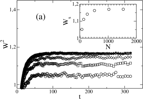
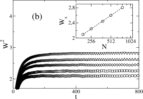
Figure 3: $W^{2}$ as a function of $t$ for the integration of the evolution equation using the linear terms and the first non-linear term in Eq. (9): $(a)\ \lambda=3.5$ for $N=64$ ($\bigcirc$), $128$ ($\Box$), $256$ ($\diamond$), $512$ ($\bigtriangleup$), $1024$ ($\bigtriangledown$) and $1536$ ($\star$). $(b)\ \lambda=2.5$ for $N=192$ ($\bigcirc$), $256$ ($\Box$), $384$ ($\diamond$), $512$ ($\bigtriangleup$), and $768$ ($\bigtriangledown$). In the inset figure we plot $W_{s}$ as a function of $N$ in symbols. The inset figure of $(b)$ is in log-linear scale and the dashed line represents the fitting with $W_{s}\sim\ln N$.

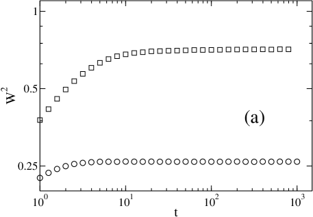
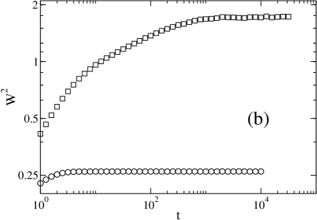
Figure 4: $W^{2}$ as a function of $t$ in log-log scale for the SRM ($\bigcirc$) and SRAM ($\Box$) models for $N=1024$ for: $(a)\ \lambda=3.5$ and $(b)\ \lambda=2.5$.

References

- [1] R. Pastor-Satorras and A. Vespignani, Phys. Rev. Lett. 86, 3200 (2001).
- [2] E. López et al., Phys. Rev. Lett. 94, 248701 (2005); A. Barrat, M. Barthélemy, R. Pastor-Satorras and A. Vespignani, PNAS 101, 3747 (2004).
- [3] Z. Wu, et al., Phys. Rev. E. 71, 045101(R) (2005).
- [4] G. Li, L. A. Braunstein, S. V. Buldyrev, S. Havlin, and H. E. Stanley, Phys. Rev. E 75, 045103(R) (2007).
- [5] J. Jost and M. P. Joy, Phys. Rev. E 65, 016201 (2001); X. F. Wang, Int. J. Bifurcation Chaos Appl. Sci. Eng. 12, 885 (2002); M. Barahona and L. M. Pecora, Phys. Rev. Lett. 89, 054101 (2002); S. Jalan and R. E. Amritkar, Phys. Rev. Lett. 90, 014101 (2003); T. Nishikawa et al., Phys. Rev. Lett. 91, 014101 (2003); A. E. Motter et al., Europhys. Lett. 69, 334 (2005); A. E. Motter et al., Phys. Rev. E 71, 016116 (2005).
- [6] G. Korniss, Phys. Rev. E 75, 051121 (2007).
- [7] J. W. Scannell et al., Cereb. Cortex 9, 277 (1999); V. M. Egu luz, D. R. Chialvo, G. A. Cecchi, M. Baliki, and A. V. Apkarian, Phys. Rev. Lett. 94, 018102 (2005)
- [8] S. Eubank, H. Guclu, V. S. A. Kumar, M. Marathe, A. Srinivasan, Z. Toroczkai and N. Wang, Nature 429, 180 (2004); M. Kuperman and G. Abramson, Phys Rev Lett 86, 2909 (2001).
- [9] H. Guclu, G. Korniss and Z. Toroczkai, Chaos 17, 026104 (2007).
- [10] A. L. Pastore y Piontti, P. A. Macri and L. A. Braunstein, Phys. Rev. E 76, 046117 (2007).
- [11] R. Albert and A.-L. Barabási, Rev. Mod. Phys. 74, 47 (2002); S. Boccaletti, V. Latora, Y. Moreno, M. Chavez and D.-U. Hwang, Physics Report 424, 175 (2006).
- [12] F. Family, J. Phys. A 19, L441 (1986).
- [13] D. D. Vvedensky, Phys. Rev. E 67, 025102(R) (2003).
- [14] A. -L. Barabási and H. E. Stanley, Fractal Concepts in Surface Growth (Cambridge University Press, New York, 1995).
- [15] C. E. La Rocca, L. A. Braunstein, and P. A. Macri, Phys. Rev. E 77, 046120 (2008).
- [16] L. K. Gallos and P. Argyrakis, Phys. Rev. E 74, 056107 (2006).
- [17] M. Catanzaro, M. Boguñá and R. Pastor-Satorras, Phys. Rev. E 71, 056104 (2005).
- [18] M. Molloy and B. Reed, Random Struct. Algorithms 6, 161 (1995); Combinatorics, Probab. Comput. 7, 295 (1998).
- [19] N. G. Van Kampen, Stochastic Processes in Physics and Chemistry, North-Holland, Amsterdam (1981).
- [20] L. A. Braunstein, R. C. Buceta, C. D. Archubi and G. Costanza, Phys. Rev. E 62, 3920 (2000).
- [21] B. Kozma, M. B. Hastings and G. Korniss, J. Stat. Mech. Theor. Exp. (2007) P08014
- [22] M. Boguñá, R. Pastor-Satorras, and A. Vespignani, Eur. Phys. J. B 38, 205 (2004).