NATURE OF HYDROGEN BOND IN WATER

Abstract

The work is devoted to the investigation of the physical nature of H-bonds. The H-bond potential $\Phi_{H}(r,\Omega)$ is studied as an irreducible part of the interaction energy of water molecules. It is defined as a difference between the generalized Stillinger–David potential and the sum of dispersive and multipole interaction potentials. The relative contribution of $\Phi_{H}(r,\Omega)$ to the intermolecular potential does not exceed $(10\div 15)\%$.

In memory of Professor Galina Puchkovskaya

1 Introduction

The simplest structure of intermolecular interaction potential is characteristic of the atomic liquids such as argon. Their intermolecular interaction potential $\Phi(r)$ is the sum of the attractive part $\Phi_{\rm dis}(r)$ caused by dispersive forces and $\Phi_{\rm rep}(r)$ that describes the repulsion:

$$\Phi(r)=\Phi_{\rm rep}(r)+\Phi_{\rm dis}(r).$$ (1)

In particular, the well-known Lennard-Jones potential has such a structure. For molecules having no spherical symmetry, the intermolecular potential becomes angular dependent [1]:

$$\Phi(r)\to\Phi(r,\Omega)=\Phi_{\rm rep}(r,\Omega)+\Phi_{\rm dis}(r,\Omega),$$ (2)

where $\Omega$ denotes the set of angles which describe the relative orientation of molecules. Such form of the intermolecular potential is characteristic of molecules N₂. For molecules without center of inversion, it is necessary to consider the dipole-dipole interaction and multipole interactions of higher order. This circumstance leads to the additional term $\Phi_{M}(r,\Omega)$:

$$\Phi(r,\Omega)=\Phi_{\rm rep}(r,\Omega)+\Phi_{\rm dis}(r,\Omega)+\Phi_{M}(r,\Omega).$$ (3)

The analogous structure of interaction potential is also inherent to molecules in water and water-alcohol solutions if their electronic shells do not overlap. At small distances between molecules, the overlapping effect of the electronic shells becomes essential. The corresponding interaction is usually called the hydrogen bond (H-bond). The intermolecular potential is represented in the form [2]

$$\Phi(r,\Omega)=\Phi_{\rm dis}(r,\Omega)+\Phi_{H}(r,\Omega),$$ (4)

where $\Phi_{H}(r,\Omega)$ includes also the repulsion and multipole interactions.

From the qualitative point of view, such a change of priorities is not justified, since the analytic continuation of multipole contributions to the overlapping region does not lead to the effects that can violate the continuity condition of the potential. That is why we should redefine the H-bond potential. In accordance with this, the H-bond potential will be defined as

$$\Phi(r,\Omega)=\Phi_{\rm rep}(r,\Omega)+\Phi_{\rm dis}(r,\Omega)+\Phi_{M}(r,\Omega)+\Phi_{H}(r,\Omega),$$ (5)

where $\Phi_{dis}(r,\Omega)$ and $\Phi_{M}(r,\Omega)$ are the analytic continuations in the overlapping region of electronic shells.

One of the most characteristic manifestations of H-bonds in liquid water and its vapor is the formation of dimers and multimers of higher order. In other words, the properties of a dimer give us the direct information about H-bonds. This fact points a way how to study the intermolecular interaction in water and, rigorously speaking, the formation of H-bonds. Let us note the main steps of this approach: 1) the interaction energy of two water molecules is described with the help of the most suitable phenomenological model potential that describes the ground state of a dimer; 2) the energy obtained in such a way is compared to that for a water dimer calculated with the help of the asymptotic multipole expansion; 3) to determine the H-bond potential, we construct the difference between the model potential and the sum of dispersive and multipole contributions. We expect that this difference will be non-zero only in a small region near the equilibrium distance between the water molecules in a dimer.

We suppose that the generalized Stillinger–David potential (GSD) [3] is the most suitable intermolecular potential for the description of the interaction between water molecules. This is a soft potential, whose parameters can change under the influence of nearby molecules. This important circumstance cannot be taken into account for almost all phenomenological potentials [7,​ 4,​ 5,​ 6,​ 8]. In contrast to the original work [9], the role of the screening functions (or overlapping effects) in GSD is taken into account more adequately. Moreover, the asymptotic behavior of the original Stillinger–David potential (SD) is corrected for large distances between molecules.

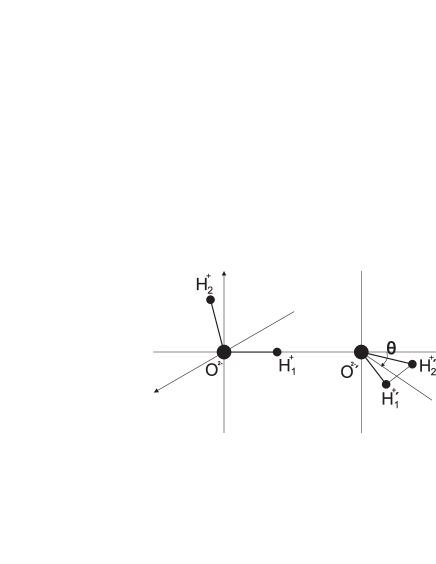
Fig. 1.: Equilibrium configuration of a water dimer

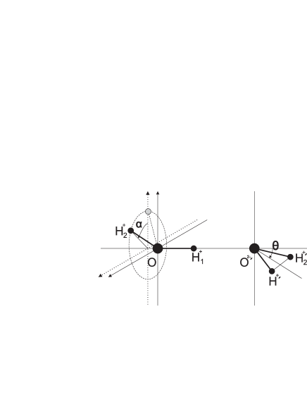
Fig. 2.: Definition of angle $\alpha$

The multipole moments (up to octupole) can be determined by the quantum-chemistry methods with sufficient accuracy [10, 11]. Due to this, we are able to construct the asymptotic estimation of the interaction potential for distances larger than the screening radius. At the same time, the analytic continuation of the multipole potential to the overlapping region does not lead to any serious errors. This allows us to construct the above-mentioned difference between the suitable model potential and multipole contribution.

The main goal of this work is the realization of the program formulated above for the construction of the H-bond potential.

2 Ground State of Water Dimer

In this section, we will represent the results of our study of dimers with the help of the GSD potential [3]. In order to facilitate the calculations, we will use the hard model of water molecules (i.e., the position of hydrogens and oxygen remain fixed, as well as their configuration). According to [3], such a requirement leads to the error of $(1.5\div 3)\%$. The ground state of a dimer is identified to the minimum of the interparticle potential for two molecules presented in Fig. 1.

The equilibrium distance $r_{\rm OO}^{(0)}$ between oxygens and the angle $\theta_{0}$ between the dipole moments of a water molecule are determined from the absolute minimum of the GSD potential: $\min\Phi_{\rm GSD}(\tilde{r},\theta,\alpha=0)$. It is considered as a function of the dimensionless distance $\tilde{r}=r_{\rm OO}/r_{\rm OH}$, where $r_{\rm OH}=0.97$ Å is the distance between the oxygen and a hydrogen in a water molecule, the angle $\theta$ describes some bend of the H-bond, and $\alpha$ is related to the rotation around the H-bond (see Fig. 2).

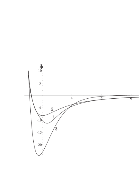
Fig. 3.: Comparative behavior of GSD potential (1), multipole potential (2), and SD potential (3)

The comparative behavior of $\Phi_{\rm GSD}$, multipole potential $\Phi_{\rm MP}$ that will be studied below, and $\Phi_{\rm SD}$ from the original work [9] is presented in Fig. 3. The equilibrium values of the distance $r_{\rm OO}^{(0)}$ between the oxygens in a dimer, the angle $\theta_{0},$ and the ground-state energy $\tilde{E}_{d}$ ($\tilde{E}_{d}=E_{d}/k_{\rm B}T_{m}$, $T_{m}$ is the melting (crystallization) temperature for liquid water, $k_{\rm B}$ is the Boltzmann constant) for all potentials investigated are presented in Table. In addition, the dipole moment $D_{d}$ of a dimer is included to Table as well. It is determined according to the formula

$$D_{d}=2d_{w}\cos\frac{1}{2}\left(\theta_{0}+\delta/2\right)\approx\sqrt{2}d_{w}\approx 2.6{\rm D}.$$ (6)

Equilibrium parameters of water dimer

Dimer parameters	$r_{\rm OO}^{(0)}$, Å	$\theta_{0}$, deg	$E_{d}$	$d_{d}$, D
GSD	3.07	31.1	–11.36	2.76
GSD($\lambda=0.98$)	3.00	18.2	–13.8	3.02
$\Phi_{\rm MP}(SD)$	3.00	26.8	–8.73	3.23
$\Phi_{\rm MP}(SP)$	3.01	27.9	–8.19	3.08
[13]	2.98	60	–10.69
[14]	2.925	47.5	–9.11
[15]			–10.32
[16]	2.976	57 $\pm$ 10
[17]				2.6

Here, $d_{w}$ denotes the modulus of the water molecule dipole moment, $\delta$ is the equilibrium angle between lines connecting oxygen and hydrogens. The second line in Table corresponds to the GSD potential, in which the screening length for the function $1-L(r)$ (see [9]) is decreased by $\lambda=0.98$ times. The dependence of the interaction energy on the rotation angle $\alpha$ around the H-bond is especially important (see Fig. 4).

As is seen, the inequality $\Delta\tilde{\Phi}(\alpha)<1$, $\Delta\tilde{\Phi}(\alpha)=\frac{\Phi(\tilde{r}_{\rm OO},\theta_{0},\alpha)-\Phi(\tilde{r}_{\rm OO},\theta_{0},0)}{k_{\rm B}T_{m}}$, indicates the possibility of intramolecular rotations of water molecules in a dimer. This circumstance should manifest itself in the entropy and heat capacity behavior [12].

3 Multipole approximation for the interparticle potential

The usage of the multipole interaction potential is justified by the following reasons: 1) multipole interaction potential of two water molecules is more convenient in specific calculations; 2) determination of multipole moments within the methods of quantum chemistry is much simpler than the construction of approximating functions; 3) comparison of the attractive part of model potentials and the electrostatic multipole potential for the dimer configuration allows us to control the degree of applicability of model potentials.

The last requirement, as it will be shown below, leads to the conclusion that the GSD potential is the most suitable for the description of water dimers.

The multipole potential of the intermolecular interaction is modeled as

$$\Phi_{\rm MP}(r)=\Phi_{0}\exp(-k(r-\sigma))+\Phi_{M}(r),$$ (7)

where the repulsion part will have the same behavior as that for the GSD [3]. Here, $\sigma$ is the doubled hard-core radius of a water molecule, which is identified as the H-bond length [2], and $\Phi_{M}(r)$ is a part of the multipole expansion for the interaction energy between two water molecules.

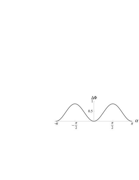
Fig. 4.: $\alpha$-dependence of the interaction energy for a dimer at $r_{\rm OO}=3$ Å

We use the multipole expansion $\Phi_{M}(r)$ up to the quadrupole-quadrupole and dipole-octupole terms:

$$\Phi_{M}(r)=\Phi_{DD}+\Phi_{DQ}+\Phi_{QQ}+\Phi_{DO}+\ldots\,.$$ (8)

For the dimer configuration in Fig. 1, the corresponding terms are

$$\Phi_{DD}=\frac{d^{2}}{r_{\rm OO}^{3}}(\cos(\delta/2+\theta)-3\cos\delta/2\cos\theta),$$

$$\Phi_{DQ}=-\frac{1}{2r_{\rm OO}^{4}}(6\{d_{\alpha}^{(1)}Q_{2\alpha}^{(2)}+d_{\alpha}^{(2)}Q_{2\alpha}^{(1)}\}-$$

$$-15\{d_{2}^{(1)}Q_{22}^{(2)}+d_{2}^{(2)}Q_{22}^{(1)}\}),$$

$$\Phi_{QQ}=\frac{3}{4r_{\rm OO}^{5}}(35Q_{22}^{(1)}Q_{22}^{(2)}-20Q_{2\delta}^{(1)}Q_{2\delta}^{(2)}+Q_{\delta\gamma}^{(1)}Q_{\delta\gamma}^{(2)}),$$

$$\Phi_{DO}=-\frac{3}{2r_{\rm OO}^{5}}(15\{d_{2}^{(1)}O_{222}^{(2)}+d_{2}^{(2)}O_{222}^{(1)}\}-$$

$$-5\{d_{\alpha}^{(1)}O_{22\alpha}^{(2)}+d_{\alpha}^{(2)}O_{22\alpha}^{(1)}\}).$$

The analysis of the repulsive part of the multipole potential shows that the parameters $\Phi_{0}$, $k$, and $\sigma$ take values $\Phi_{0}=8.5$, $k=5$, and $\sigma=2.8$. The relative values of different contributions to $\Phi_{M}$ are shown in Fig. 5. Lines (3) and (4) testify that the quadrupole-quadrupole and dipole-octupole interactions have the same order of magnitude.

As is seen from Fig. 3, the multipole part is able to correctly describe the interaction energy at distances up to $4$ Å. More exactly, on the interval $4$ Å $<r_{\rm OO}<\inf,$ the values of multipole potential and GSD coincide with high accuracy. At smaller distances between oxygens, the overlap of electronic shells begins. The multipole approach becomes inapplicable. At the same time, the phenomenological model potentials are supposed to be used also in this region. In particular, the applicability of the GSD potential within the overlapping region is justified by a suitable selection of the screening functions. Unfortunately, the most of other phenomenological potentials have no necessary compliance. The generalized Stillinger–David potential, used in our consideration of dimer properties, is quite satisfactory, and it has the ability for further modifications.

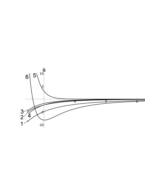
Fig. 5.: Role of the terms $\Phi_{DD},\,\Phi_{DQ},\,\Phi_{QQ}$, and $\,\Phi_{DO}$ in the multipole interaction potential (7) of two water molecules in the dimer configuration: 1 – $\Phi_{DD}$, 2 – $\Phi_{DQ}$, 3 – $\Phi_{QQ}$, 4 – $\,\Phi_{DO}$, 5 – $\Phi_{\rm rep}$, 6 – $\Phi_{\rm MP}$

4 Hydrogen Bond Potential

According to the definition of H-bond given in Introduction, we will consider the difference $\Phi_{H}(r)$ between the generalized Stillinger–David potential $\Phi_{\rm GSD}$ and the sum of the multipole potential $\Phi_{M}$ and the dispersive energy [8]:

$$\Phi_{H}(r,\Omega)=\Phi_{\rm GSD}(r,\Omega)-\Phi_{r}(r,\Omega)-\Phi_{\rm dis}(r,\Omega)-\Phi_{\rm MP}(r,\Omega).$$ (9)

The behavior of the potentials $\Phi_{\rm GSD}(r,\Omega)$, $\Phi_{\rm dis}(r,\Omega),$ and $\Phi_{\rm MP}(r,\Omega)$ for the configuration of molecules characteristic of a dimer is presented in Fig. 6.

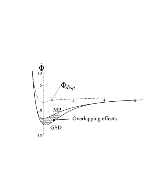
Fig. 6.: Partial contributions to the intermolecular potential.

The H-bond potential for the same configuration is presented in Fig. 7.

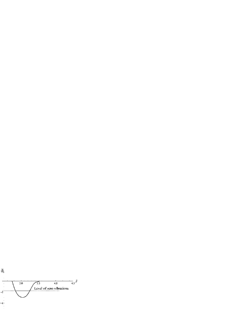
Fig. 7.: H-bond potential.

Hence, $\Phi_{H}(r,\Omega)$ is a short-range potential that appears due to the overlapping of the electronic shells, and it has the quantum mechanical nature. It should be interpreted as an H-bond potential in water. It takes the same order of magnitude as the dispersive term and is much smaller than the multipole interaction ($\Phi_{\rm dis}\leavevmode\nobreak\ (1\div 2)k_{\rm B}T_{m}$, $\Phi_{\rm MP}\leavevmode\nobreak\ (7\div 8)k_{\rm B}T_{m}$, $\Phi_{H}\leavevmode\nobreak\ (2\div 3)k_{\rm B}T_{m}$). That is why the contribution of H-bonds to the thermodynamic potential can be taken into account with the help of perturbation theory. This circumstance is confirmed qualitatively by the similarity of thermodynamic properties of water and argon on their coexisting curves [19].

5 Discussion

The relatively small depth of the potential well of a hydrogen bond leads to the following conclusions: 1) contributions of $\Phi_{H}(r,\Omega)$ to the thermodynamic potentials and the kinetic coefficients can be calculated with the help of perturbation theory; 2) temperature behavior of the thermodynamic characteristics such as the fraction volume or the heat of evaporation is argon-like with satisfactory accuracy. The last conclusion is confirmed by the results from [18–20]. The H-bond potential in Fig. 7 corresponds to the equilibrium orientation of water molecules. There are no restrictions to construct $\Phi_{H}(r,\Omega)$ for all other orientations: all angular dependences of $\Phi_{\rm GSD}(r,\Omega)$ and $\Phi_{\rm MP}(r,\Omega)$ are well known. However, we have to mention that the thermodynamic properties of water are defined by the averaged intermolecular potential due to the rotation of water molecules [20]. It is shown [20] that the potential well depth reduces due to the averaging over angular variables. This leads to the correction of the argon-like dependences of thermodynamic quantities by at most $5\%$ [18, 20]. Nevertheless, the contributions of H-bonds exhibit themselves in the heat capacity of water [12], dipole relaxation, and spectral properties [2]. Another important circumstance is the necessity to consider the influence of the neighbors on the H-bond potential. This collective effect will be studied in details in further publications.

The authors cordially thank Prof. V. Balevicius, Prof. L. Kimtys, Prof. A. Koll, Prof. A.V. Kraiski, Prof. N.I. Lebovka, Prof. L.N. Lisetskiy, Prof. N.N. Melnik, and especially Prof. V.E. Pogorelov for the fluidful discussion of the results obtained.

ПРИРОДА ВОДНЕВОГО ЗВ’ЯЗКУ У ВОДI
П.В. Махлайчук, М.П. Маломуж, I.В. Жиганюк
Р е з ю м е
Роботу присвячено дослiдженню фiзичної природи водневого зв’язку, який утворюється мiж молекулами води. Потенцiал водневого зв’язку $\Phi_{H}(r,\Omega)$ розглядається як незвiдна частина енергiї взаємодiї молекул води, що визначається рiзницею мiж узагальненим потенцiалом Cтiлiнджера та Девiда i сумою потенцiалiв дисперсiйної та мультипольної взаємодiй. Показано, що вiдносна величина внеску $\Phi_{H}(r,\Omega)$ не перевищує (10–15)%.

References

- [1] C.A. Croxton, Liquid State Physics. A Statistical Mechanical Introduction (Cambridge Univ. Press, Cambridge, 1974).
- [2] D. Eisenberg and W. Kauzmann, The Structure and Properties of Water (Oxford Univ., New York, 1969).
- [3] I.V. Zhyganiuk, Ukr. J. Phys. 56, 225, (2011).
- [4] V.Ya. Antonchenko, A.S. Davydov, and V.V. Il’in, Foundations of the Physics of Water (Naukova Dumka, Kiev, 1991) (in Russian).
- [5] J.D. Bernal and R.H. Fowler, J. Chem. Phys. 1, 515 (1933).
- [6] A. Rahman and F.H. Stillinger, J. Chem. Phys. 55, 3336 (1971).
- [7] W.L. Jorgensen, J. Chandrasekhar, and J.D. Madura, J. Chem. Phys. 79, 926 (1983).
- [8] V.I. Poltev, T.A. Grokhlina, and G.G. Malenkov, J. Biomolec. Struct. Dynam. 2, 413 (1984).
- [9] F.H. Stillinger and C.W. David, J. Chem. Phys. 69, 1473 (1978).
- [10] I.G. John, G.B. Bacskay, and N.S. Hush, Chem. Phys. 51, 49 (1980).
- [11] D. Neumann and J.W. Moskowitz, J. Chem. Phys. 49, 5 (1968).
- [12] S.V. Lishchuk, N.P. Malomuzh, and P.V. Makhlaichuk, Phys. Lett. A 375, 2656 (2011).
- [13] H. Umeyama and K. Morokuma, J. Amer. Chem. Soc. 99, 1316 (1977).
- [14] M. Schütz, S. Brdarski, P.-O. Widmark, R. Lindh, and G. Karlström, J. Chem. Phys. 107, 4597 (1997).
- [15] O. Matsuoka, E. Clementi, and M. Yoshimine, J. Chem. Phys. 64, 1351 (1976).
- [16] J. Odutola and T.R. Dyke, J. Chem. Phys. 72, 5062 (1980).
- [17] H. Yu and W.F. Gunsteren, J. Chem. Phys. 121, 9549 (2004).
- [18] L.A. Bulavin, A.I. Fisenko, and N.P. Malomuzh, Chem. Phys. Lett. 453, 183 (2008).
- [19] A.I. Fisenko, N.P. Malomuzh, and A.V. Oleynik, Chem. Phys. Lett. 450, 297 (2008).
-
[20]
S.V. Lishchuk, N.P. Malomuzh, and P.V. Makhlaichuk, Phys. Lett. A 374, 2084 (2010).
Received 10.10.11