The kinetic temperature in a damped Lyman-alpha absorption system in Q2206 – 199 - an example of the warm neutral medium

Abstract

By comparing the widths of absorption lines from O 1, Si 2 and Fe 2 in the redshift $z_{\rm abs}=2.076$ single-component damped Ly$\alpha$ system in the spectrum of Q$2206-199$ we establish that these absorption lines arise in Warm Neutral Medium gas at $\sim 12000\pm 3000$ K. This is consistent with thermal equilibrium model estimates of $\sim 8000$ K for the Warm Neutral Medium in galaxies, but not with the presence of a significant cold component. It is also consistent with, but not required by, the absence of C 2 fine structure absorption in this system. Some possible implications concerning abundance estimates in narrow-line WNM absorbers are discussed.

1 Introduction

The complex structure of the interstellar medium in the Galaxy may be considered as a mixture of four components: the neutral atomic hydrogen is found to be generally in cold neutral medium (CNM, $\mathrel{\hbox to0.0pt{\lower 3.0pt\hbox{$\mathchar 536\relax$}\hss}\raise 1.5pt\hbox{$\mathchar 316\relax$}}500$ K) and warm neutral medium (WNM, $\sim 5000$ - $10000$ K) gas (Wolfe, Prochaska & Gawiser, 2003), and ionized material may be warm (WIM, $\sim 10^{4}$ K) or hot (HIM, $T\sim 10^{6}$ K) (McKee & Ostriker, 1977). The WNM and CNM are expected to be in approximate pressure balance (e.g. Wolfire et al., 1995); H 1 at temperatures between the two is unstable and will rapidly evolve towards one of the two stable states. The CNM and WNM are usually studied using H 1 21cm absorption against background radio sources, and show that a significant fraction of the warm material may be in the unstable regime (see the discussion by Wolfire et al., 1995, also Begum et al., 2010).

Temperature estimates for Damped Lyman-alpha absorption systems (DLAs) reveal both CNM and WNM gas. The presence of C 2 fine structure absorption is associated with the CNM (Wolfe, Prochaska & Gawiser, 2003; Wolfe, Gawiser & Prochaska, 2003), and Howk, Wolfe & Prochaska (2005) use C 2 and Si 2 fine structure lines to show that a system at redshift $z=4.2$ contains CNM material. Lehner et al. (2008) use an upper limit to the C 2^∗ column density in the $z=2.377$ DLA to show that the neutral gas in this system must be warm. Modelling of a few weak Mg 2 absorbers also suggests temperatures of $\sim 10000$ K (Jones et al., 2010). From 21cm spin temperature studies Kanekar et al. (2009) suggest that a significant fraction of the H 1 at redshifts $z>1.6$ is warm. However, this conclusion is controversial as it requires assumptions about the temperature and density distribution of the gas across the  100 pc dimensions of the background radio sources that have not been demonstrated (Wolfe et al., 2011).

The few attempts to estimate temperatures from the line widths in DLAs have relied on the identification of narrow absorption components, normally from C 1, which show up clearly as distinct sharp features (Jorgenson et al., 2009; Tumlinson et al., 2010; Carswell et al., 2011). The corresponding temperatures of a few hundred degrees Kelvin or less indicate that the absorbing gas is in a cold neutral medium (CNM). However, attempts to determine temperatures by using the widths of singly ionized heavy element lines have not been very successful, either in the Galaxy (Nehmé et al., 2008) or at higher redshifts (Carswell et al., 2011) because of uncertainties introduced by the blending of many velocity components. One exception is for the interstellar medium near the Sun, where Redfield & Linsky (2004) find temperatures averaging 6800K with a dispersion of $\sim 1500$ K.

One way of avoiding velocity component confusion is to select systems for which the velocity structure in the singly ionized species is simple. These are rare, and may not be typical, but it is of interest to see if the inferred temperature in such cases is $\sim 8000$ K, as would be expected for the WNM (Wolfire et al., 1995), or if a temperature of $\mathrel{\hbox to0.0pt{\lower 3.0pt\hbox{$\mathchar 536\relax$}\hss}\raise 1.5pt\hbox{$\mathchar 316\relax$}}500$ K typical of the CNM is more appropriate. The other requirements are that at least two ion species with different atomic masses and transitions with a range of oscillator strengths be measured, and that at least some of these fall on different parts of the curve of growth (normally linear and logarithmic) so that the Doppler parameters for the ions may be estimated individually (Jorgenson et al., 2009; Carswell et al., 2011).

There are two studies where the inferred line widths have yielded temperature estimates in QSO absorbers dominated by single-component systems with strong H 1, both as part of D/H abundance studies. O’Meara et al. (2001) use Keck HIRES spectra to derive a temperature $T=1.15\pm 0.02\times 10^{4}$ K, and a bulk motion component $b_{\rm turb}=2.56\pm 0.12$ km s^-1 by comparing the Doppler parameters for the H 1, N 1 and O 1 lines in a system with H 1 column density $\log N({\rm\text{H\,{1}}})=19.42$ at redshift $z=2.536$ towards the QSO HS$0105+1619$. The other is a DLA at redshift $z=2.076$ in the spectrum of Q$2206-199$ which was studied by Prochaska & Wolfe (1997) using Keck HIRES data. Pettini & Bowen (2001) used a combination of HST STIS and VLT UVES data to derive a similar, if less certain, temperature by comparing the Doppler parameters for H 1 and singly ionized heavy element lines.

We revisit the second case here, since the temperature is based largely on low S/N STIS spectra for higher order Lyman lines. With the presence of several transitions of a range of ions of different masses, O 1, Si 2 and Fe 2 there is the prospect of temperature estimation from the heavy element lines alone. In the next section we describe the spectroscopic data and the techniques used to establish a temperature $T\sim 12000\pm 3000$ K. Section 2.3 describes a series of tests undertaken to ensure that the result is reliable, and in particular that the error range is realistic and that the absorbing medium must be warm, and some further temperature indicators are considered in Section 2.4. Section 3 examines some implications of the temperature estimate, particularly for relative element abundance estimates in cases where the absorption lines are intrinsically narrow, and the main conclusions are summarized in Section 4.

2 The redshift 2.076 absorption system in Q2206 – 199

2.1 The data

The absorption system at redshift $z=2.076$ in Q$2206-199$ was found to have low heavy element abundances, with ${\rm[Si/H]}\mathrel{\hbox to0.0pt{\lower 3.0pt\hbox{$\mathchar 536\relax$}\hss}\raise 1.5pt\hbox{$\mathchar 316\relax$}}-2.4$, by Rauch et al. (1990) using 30 km s^-1 resolution spectra. Using higher resolution Keck HIRES spectra, Prochaska & Wolfe (1997) noted the very low Fe 2 and Al 2 abundances in a system at redshift $z=2.076214$, and that the system appeared to have only a single velocity component. Prochaska et al. (2001) re-examined this system and further determined the abundance for Si 2, further confirming it as a low abundance system with ${\rm[Fe/H]}=-2.6$, and ${\rm[Si/H]}=-2.3$.

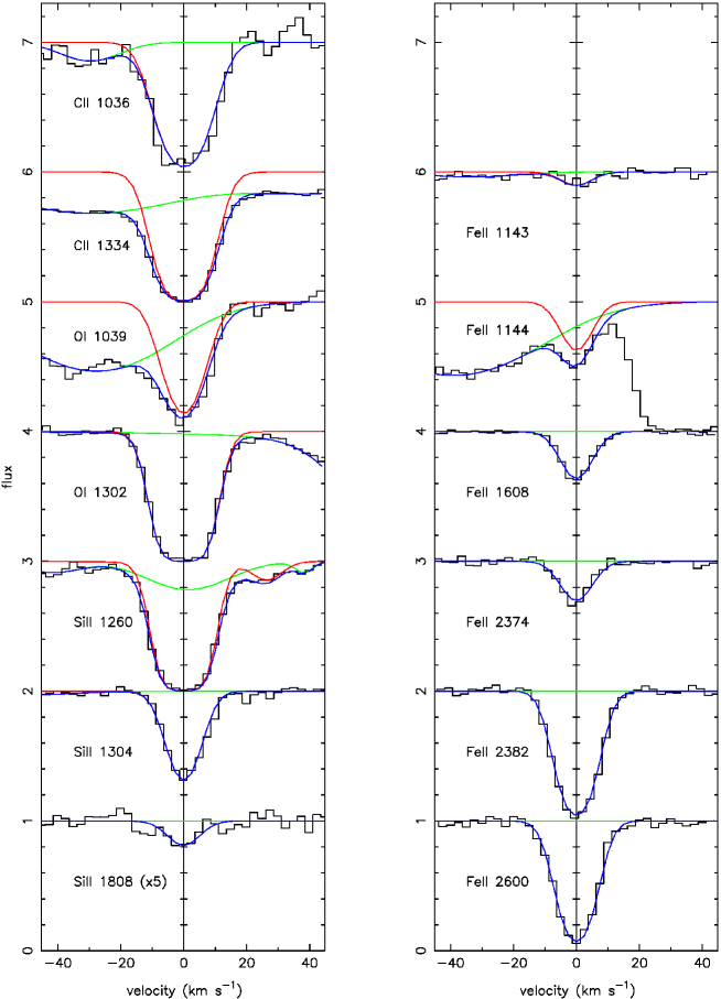
Figure 1: The Voigt profile fits and data for the C 2, O 1, Si 2 & Fe 2 lines used on a velocity scale relative to redshift $z=2.0762286$. The data are shown as black histograms and the overall fits in blue. Where they differ from the overall fitted profiles, the fits to the transitions of interest here are indicated are shown in red, and any interlopers shown in green. All but Si 2 1808 are shown against a unit continuum, and the continua for different lines have been separated by an integer offset. The Si 2 1808 line is weak, and has been scaled up by a factor of five so it can be seen more clearly. The dip (in red) at $+26$ km s^-1 relative to the Si 2 1260 line is Fe 2 1260 at the same redshift.

The spectra used here were obtained using UVES on the ESO VLT, for programmes 65.O-0158(A) (Pettini et al., 2002), 072.A-0346(A) (Petitjean et al., 2006) and 074.A-0201(A). For each exposure ESO provides a seeing estimate from their differential image motion monitor. The standard setting DIC2 437 (3730 - 4990 Å) & 860 (6650 - 10600 Å) was used for two exposures for a total of 7800s in 0.5 arcsec seeing as part of programme 65.O-0158(A). The other settings used in that programme were DIC1 390 (3260 - 4450 Å) & 564 (4580 - 6680 Å), for 10800s with 0.5 arcsec seeing and 6300s with slit-limited (1 arcsec) resolution. For programme 072.A-0346(A) the seeing approximately matched the slit width of 1 arcsec, and the exposures totalled 9000s for DIC1 346 (3030 - 3880 Å) & 580 (4760 - 6840 Å) settings. Programme 074.A-0201(A) used a 0.9 arcsec slit in seeing ranging from 0.8 to 1.1 arcsec with total exposure times of 19603s in settings DIC2 455 (3930 - 5160 Å) & 850 (6580 - 10420 Å). The data were reduced using the UVES pipeline and the UVES_popler package. The signal-to-noise ratio (S/N) in the coadded spectrum is 60 per 2.5 km s^-1 pixel at 5000 Å.

Table 1: Q$2206-199$ $z=2.076$ system profile fit parameters.

Ion	$z$	$\pm$	$b$	$\pm$	$\log(N)$	$\pm$	$b_{\rm turb}$	$\pm$	$T$ (K)	$\pm$
C II	2.0762286	0.0000005	7.66	0.26	14.24	0.03
O I			6.43	(0.16)	15.08	0.05	5.3	0.2	$1.22\times 10^{4}$	$3.2\times 10^{3}$
SiII			5.99	(0.14)	13.69	0.01
FeII			5.68	(0.11)	13.35	0.01
??	2.1898787	0.0000107	2.23	2.28	11.67	0.14
H I	1.6221834	0.0000260	12.22	4.92	12.43	0.15
H I	1.6290246	0.0000890	26.68	12.25	12.69	0.22
H I	1.6295216	0.0000189	28.39	4.02	13.46	0.07
H I	1.8925871	0.0000713	18.38	15.79	12.00	0.55
H I	1.8968634	0.0000063	33.22	3.24	13.57	0.07
H I	2.1890279	0.0000208	12.42	3.05	12.18	0.09
H I	2.1894871	0.0000125	17.10	3.12	12.76	0.10
H I	2.2958922	0.0000256	10.88	3.14	12.85	0.20
H I	2.2959933	0.0000046	24.56	0.55	13.85	0.02
H I	2.2968227	0.0000682	98.83	10.40	13.46	0.06
H I	2.2977042	0.0000065	20.64	0.53	13.95	0.02
H I	2.2980854	0.0000359	18.28	2.54	12.97	0.11
H I	2.2998674	0.0000571	35.49	11.59	12.43	0.21
H I	2.3766727	0.0000325	39.47	4.17	13.30	0.05
H I	2.3774852	0.0000461	31.52	8.53	12.85	0.13

Column densities $N$ have units cm^-2, and Doppler parameters $b$ are in km s^-1.

‘??’ denotes an unidentified line, taken to have the same rest wavelength and oscillator strength as Ly$\alpha$.

The variety of slit widths and wavelength settings is likely to result in the spectral resolution being a function of wavelength. For individual exposures appropriate width Gaussians provide an adequate approximation to the instrument profile. For the slit-limited cases, which dominate the final sum here, we verified this assumption by establishing that single Gaussians gave good fits to night sky emission lines in the sky spectrum described by Hanuschik (2003). For the seeing-limited observations there may be extended wings beyond a core which is reasonably close to a Gaussian (see e.g. Diego 1985, King 1971). We have constructed an instrument profile as a sum of Gaussians with a common centre and with widths determined using the resolution - slit width product $R\times s=41400$ ($s$ in arcsec) for the blue arm and $R\times s=38700$ for the red arm of the spectrograph, weighting each by the relative efficiency (see the ESO UVES instrument characteristics webpage and the response curves linked to from there). For the 0.5 arcsec seeing-limited exposures we took $s$ to be the seeing estimate. For the other exposures the resolution was close to being slit-limited, so $s$ was set to the appropriate slit width. While for the seeing limited exposures the adopted profile will not give the full description, any flux outside the core will be dominated by the slit-limited observations so should not be important. In any case, as we show below, the results here are insensitive to the line-spread-function adopted so a precise one is not needed.

The error estimates provided by the data extraction package were found to be close to those inferred by examining the root-mean-square (RMS) deviations in continuum regions. However, in lines which have zero residual intensity the RMS measures indicated that the error estimates were too low by a factor of 2. We verified that this is generally true for UVES spectra extracted in this way by examining data for other objects. To correct for the error underestimate when the data is near zero we multiplied the error term by $\left(1.0+15.0\times{\rm min}\left(1.0,{\rm max}\left(0.0,(1.0-d_{i}/c_{i})\right)^{4}\right)\right)^{1\over 4}$, where $d_{i}$, $c_{i}$ are the data and continuum values in the $i$th data pixel. While it is not clear what the true correction should be, this function was chosen because it changes the error little when the data is not close to zero and doubles it near zero intensity. Provided that the correction is sharply peaked near the data zero, the precise form of the correction makes little difference to the results here.

2.2 Temperature estimation

The full optical wavelength coverage of these spectra allows us to measure several Fe 2 and Si 2 lines with a range of oscillator strengths $f$ and wavelengths $\lambda$, and O 1 1039 and 1302 with $f\lambda$ values differing by 0.8 dex. So, at least in principle, we may estimate the Doppler parameters for these species independently. Also, with a range of $f\lambda$ values the profile fits depend most strongly on the curve of growth, and not on an estimate of the instrument profile (Carswell et al., 2011). We assume that all ions arise predominantly in the same region where a single temperature is appropriate. Since they arise in a DLA these assumptions should be close to reality. Within the region we assume that the Doppler parameter for a given ion is $b=\sqrt{b_{\rm turb}^{2}+2kT/m}$, where $b_{\rm turb}$ is the turbulent (bulk) component, $k$ Boltzmann’s constant, $m$ the ion mass and $T$ the temperature. We used the VPFIT program with oscillator strengths from the compilation by Morton (2003). For the Doppler parameters $b_{\rm turb}$ and $T$ were used as the independent variables for at least two ions of different mass at the same redshift simultaneously, with the constraints that both variables are non-negative. The error estimates from the program then apply to $b_{\rm turb}$ and $T$, not to the Doppler parameters for the individual ions. The temperature component of the Doppler width varies as $1/\sqrt{m}$, so even for O 1 and Fe 2 the thermal widths differ by less than a factor of two and for other available ions the ratio is even smaller. If there is a significant turbulent component then the differences in the line widths could be quite small. Under these circumstances, even quite well-determined Doppler parameters for individual ions can yield large error estimates for both $b_{\rm turb}$ and $T$. The Doppler parameter error estimates shown in parentheses in Table 1 are given as a guide only, and were obtained by assuming that the $b$-value for each ion was determined independently of the others.

The redshifts of C 2 1036 and 1334 were tied to be the same as for the other ions to provide a (small) increase in the precision of the $z$-estimate. However, since the C 2 $f\lambda$ values differ by only 0.14 dex they were not used for constraining the temperature. The N 1 lines at 1200 Å are too weak to be useful.

In the $z=2.076$ absorption system Si 2 1260, 1304 and 1808 are reasonably clear of contaminating absorption lines from systems at other redshifts, but Si 2 1526, which is clear of the Ly$\alpha$ forest, is unusable because it is badly blended with a strong complex Fe 2 1608 at redshift $z=1.9205$. Allowance has to be made for blended Ly$\alpha$ forest lines for all usable Si 2 lines except 1808. This is straightforward generally, since the Ly$\alpha$ lines are significantly broader than the heavy element ones. Some of the longer wavelength Fe 2 lines are affected by atmospheric absorption and emission, but Fe 2 1608, 2374, 2382 and 2600 are clear of serious contamination. At shorter wavelengths Fe 2 1260 is in the wing of Si 2 1260, and Fe 2 1143 and 1144 provide useful constraints. For O 1 1302 and 1039 are also useful, though the 1039 line is blended with a broad Ly$\alpha$. The results of fitting these with VPFIT are given in Table 1, along with the blends fitted at the same time. The Doppler parameters for O 1, Si 2 and Fe 2 were determined using common values of $b_{\rm turb}$ and $T$, which were treated as independent variables. The error estimates for the Doppler parameters given in brackets are derived assuming that they are independent of those for the other ions. The line designated by ‘??’, which is assigned the same wavelength and oscillator strength as Ly$\alpha$, is a marginal narrow component which is probably an unidentified heavy element.

There are two data uncertainties which should be allowed for. The continuum level cannot be determined precisely, especially in the Ly$\alpha$ forest, and inaccurate continuum levels can cause inconsistencies when several lines of the same ion are fitted simultaneously. The other is the true zero level for the data, which can affect strong lines particularly, can differ from the data extraction zero by 1 or 2%. The VPFIT package allows both of these to be used as further free parameters in the overall fit, and we have done so where necessary. We do not give their values in Table 1 since they depend on how well the continuum and zero levels have been estimated originally.

From Table 1 we see that the temperature estimate for the system is $T={\color[rgb]{0.00,0.00,0.00}1.22}\pm 0.32\times 10^{4}$ K, so consistent with it being WNM but not CNM. The turbulent component of 5.3 km s^-1 is larger than the thermal broadening for any of the ions at the inferred temperature. For O 1 the thermal width is $b={\color[rgb]{0.00,0.00,0.00}3.5}$ km s^-1, for Si 2 2.7 km s^-1 and for Fe 2 1.9 km s^-1. However, these thermal widths are enough to give measurable differences in the Doppler parameters for the ions involved.

Table 2: Other $z=2.076$ system ions

Ion	$z$	$\pm$	$b$	$\pm$	$\log(N)$	$\pm$
H I	2.0762286	(0.0000005)	15.19	-	20.44	0.05
C II	2.0762286		6.75		14.35	0.02
C II∗	2.0762286		6.75		$<12.75$	($2\sigma$)
AlII	2.0762286		6.01		12.17	0.01
AlIII	2.0762286		6.01		11.46	0.06
C IV	2.0753686	0.0000121	7.54	1.88	12.09	0.08
C IV	2.0761144	0.0000058	5.11	1.49	12.67	0.20
C IV	2.0762127	0.0000286	17.32	2.09	13.57	0.04
C IV	2.0764230	0.0000136	9.57	1.87	13.00	0.22
C IV	2.0766579	0.0000409	12.42	5.11	12.24	0.17
SiIV	2.0761218	0.0000020	7.75	0.33	12.64	0.02
SiIV	2.0764017	0.0000065	12.91	1.05	12.55	0.03

Note: H 1, C 2, Al 2 and Al 3 redshifts and $b$-values are obtained from the parameters given in Table 1.

The C 2 column density given in Table 1 is the best fit obtained by leaving its Doppler $b$ to be determined independently of the other ions. If we impose the turbulent component and temperature derived above, then for C 2 $b=6.75$ km s^-1 and $\log N=14.38\pm 0.03$ (see Table 2).

For the fitted profiles given in Table 1 the reduced $\chi^{2}=1.103$ ($\chi^{2}=893.39$ for 810 degrees of freedom). The formal probability that this fit describes the data is 0.022. One might improve the fit by adding more blended lines, but the the reduction in $\chi^{2}$ is to some extent offset by the loss in the number of degrees of freedom - see Rauch et al. (1992) for a discussion on this point. We have not quite reached that stage: the temperature estimate does depend on having identified all the narrow ($<10$ km s^-1) blends with key lines. For example, adding an extra narrow component to Si 2 1304 gives a system temperature of 11800 K. However, the Si 2 1260 profile suggests that this narrow component is not Si 2, and we have not found any other lines in a system which would plausibly identify such a component.

For this system the H 1 column density is $\log N({\rm\text{H\,{1}}})=20.43\pm 0.06$ (Pettini et al., 1994; Prochaska et al., 2001). Pettini et al. (1994) show a fit to the Ly$\alpha$ profile. From the UVES data we obtain a very similar result ($\log N({\rm\text{H\,{1}}})=20.44\pm 0.05$, with the error dominated by systematic effects). However, it is difficult to be sure of the continuum over the damped Ly$\alpha$ profile in the echelle spectrum so we adopt the Pettini et al. (1994) and Prochaska et al. (2001) value.

That the singly ionized species do arise in a neutral region, so with the temperature established above, in the WNM, is strongly indicated by the fact that it is the only component which is likely to give rise to the damped Ly$\alpha$ line. Further, the corresponding Al 3 lines are weak, and from Table 2 the Al 3/Al 2 ratio is $-0.7$ dex, so the singly ionized species dominates. There is also no sign of a significant component of Si 4 at the Si 2 redshift, though it would fall between the two Si 4 components given in the table. There is a C 4 component at a redshift which, within the rather large errors, is consistent with the low ionization redshift. However the Doppler parameter is high so it is unlikely to be closely associated with the region of interest.

If the ionization correction is negligible for the low ionization component, then the abundances relative to the solar photosphere (Asplund et al., 2009) are ${\rm[Fe/H]}=-2.59\pm 0.06$, ${\rm[Si/H]}=-2.29\pm 0.06$ and ${\rm[O/H]}=-2.28\pm 0.08$. Using the turbulent-plus-thermal value for the Doppler parameters, ${\rm[C/H]}=-2.64\pm 0.06$, so ${\rm[C/O]}=-0.36$. These abundances and column densities are consistent with those given by Pettini et al. (2008), who assumed a common Doppler parameter of $b=6.5$ km s^-1 for all ions. The Fe 2 and Si 2 values are also similar to those reported for this system by Prochaska & Wolfe (1997); Prochaska et al. (2001).

2.3 Is the result reliable?

The temperature estimate here is 12200K, but the VPFIT error estimate of 3200K is large, so at the $1\sigma$ level ${\color[rgb]{0.00,0.00,0.00}9\times 10^{3}<T<1.54\times 10^{4}}$K. When the errors are roughly comparable with the best estimate value one might be concerned at the reliability of the error estimate, since e.g. negative temperatures are unphysical. This is not quite the case here, but to further check we have generated artificial spectra using the best-fit parameters given in Table 1, convolved these spectra with the appropriate instrument profiles, added noise to mimic that in the original data, and determined the fit parameters from these spectra using the same fit regions and allowance for continuum and zero level adjustments as we did for the original data. From 2000 trials we find that the mean fitted temperature is $12270$ K, with a standard deviation of $3350\pm 55$ K. The expected error in the mean temperature estimated from the 2000 trials is then $3350/\sqrt{1999}=75$ K. This mean temperature is therefore not significantly different from the input value, while the standard deviation is a little higher than the mean VPFIT estimate of 3200 K.

Another way of checking the results is to derive the best fit $\chi^{2}$ values for a range of assumed temperatures $T$, and then use the values of $\Delta\chi^{2}(T)=\chi^{2}(T)-\chi^{2}_{\rm min}$ to estimate the error ranges. The method is described by Lampton, Margon & Bowyer (1976). In the application here we have at least two closely correlated (or anti-correlated) variables, the temperature and the turbulent Doppler parameter, so for a given probability $P$ we look for the temperature range for which $\Delta\chi^{2}(T)$ is less than the value of $\chi^{2}$ corresponding to $P$ for two degrees of freedom. Under this assumption, for a degree of confidence of 68.3% ($1\sigma$ for a normal distribution) $\Delta\chi^{2}(T)<2.3$, and for a $<2\sigma$ deviation for a two-sided threshold) $\Delta\chi^{2}(T)<6.2$. The results are shown in Fig. 2, from which it is evident that the best fit value for the temperature is in good agreement with that obtained from VPFIT, but the $1\sigma$ error estimates from this method, $\pm 3900$ K, are a little pessimistic, with those from this procedure being a little over $\sim 15\%$ larger than those from the simulations.

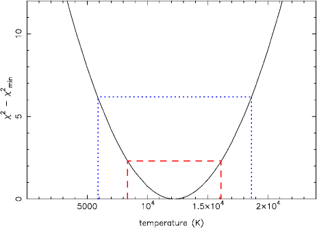
Figure 2: Voigt profile fit $\chi^{2}$ values as a function of temperature from fits to O 1, Si 2 & Fe 2 lines. The dashed lines show the $\Delta\chi^{2}$ level for the $1\sigma$ range, and the dotted lines for $2\sigma$, for two degrees of freedom. The $\chi^{2}_{\rm min}$ value is 893.39 (811 d.f.).

These analyses preclude the possibility that a significant amount of the absorption arises in cold gas. If we take 1000 K as a somewhat generous upper limit for CNM gas, then using the Doppler parameters are almost but not quite the same for the three ions, we find $\Delta\chi^{2}={\color[rgb]{0.00,0.00,0.00}18.86}$. The formal probability of this occurring by chance is ${\color[rgb]{0.00,0.00,0.00}1.4\times 10^{-5}}$.

Another way of establishing the probability that the material is WNM rather than CNM is to generate synthetic spectra with the best-fit parameters for an assumed temperature of 1000 K, which we take as the upper limit for the CNM. These were $\log N($O 1$)=15.23$ (cm^-2) with $b($O 1$)=5.99$ km s^-1, $\log N($Si 2$)=13.69$, $b($Si 2$)=5.95$ km s^-1 and $\log N($Fe 2$)=13.36$, $b($Si 2$)=5.93$ km s^-1. As in the simulations described above, we convolved these synthetic spectra with the appropriate instrument profiles, added noise to mimic that in the original data, and determined the fit parameters from these spectra using the same fit regions and allowance for continuum and zero level adjustments as we did for the original data. We also did this for 2000 trials, and find in only one case was the fitted temperature above 10000 K, with none above 11000 K. Since our temperature estimate was 12200 K, we conclude that the probability that we are observing CNM gas is $<0.0005$.

Since we have chosen lines which sample different parts of the curves of growth we do not expect that our results will depend strongly on the chosen instrument profile. However, since the absorption lines are resolved there could be some dependence on its assumed shape and width. We have undertaken some tests and find that this is not an important consideration. These were:

1. As a first check we note that for lines in the rest wavelength range 1140 - 1350 Å and for Si 2 1808 the seeing limited ($\sim 0.5$ arcsec) and slit limited ($\sim 1$ arcsec) exposure times were comparable, in the range 1.2:1 to 0.7:1. For Fe 2 1608, the Fe 2 lines above 2300 Å, and O 1 1039 the ratio is $\sim 0.5$:1 or less. Since the inferred Doppler parameter for Fe 2 is the lowest and most of the lines used in its determination have the broadest instrument profiles, it suggests that the raw instrument profile is not propagating directly into the inferred line widths.

2. We have further checked that the temperature estimate is largely independent of the assumed instrument profile by performing the Voigt profile fits with different weights for the 0.5:1 arcsec components. We also used single Gaussian point-spread functions for the whole spectrum, with widths ranging from 4.0 - 8.0 km s^-1 FWHM. While the details changed, and at the ends of the Gaussian ranges the fits were not really acceptable, the temperature estimate proved robust with $11000<T<13000$ K. The error estimates were similar in all cases, at $\mathrel{\hbox to0.0pt{\lower 3.0pt\hbox{$\mathchar 536\relax$}\hss}\raise 1.5pt\hbox{$\mathchar 316\relax$}}3600$ K.

While the narrow lines in the Ly$\alpha$ forest are easily separable from the broad Lyman lines, the effective continuum for these narrow lines is affected by the Ly$\alpha$ absorption. The fitting procedure does take account of the additional uncertainties given the fit model, but, since the O 1 1039 line is strongly blended with Ly$\alpha$, as a rough consistency check we have refitted using only Si 2 and Fe 2 to estimate the temperature. Not surprisingly, since the total ion mass range is lower by almost a factor of two, the error estimates increased significantly. We obtained $b_{\rm turb}=5.2\pm 0.3$ km s^-1and $T=1.7\pm 0.7\times 10^{4}$ K. So the best fit is at a higher temperature, but without the O 1 the significance level for the material to be in the WNM rather than the CNM falls to $2.3\sigma$.

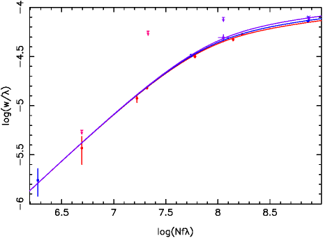
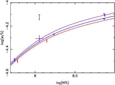
Figure 3: Curves of growth using the fitted Doppler parameters given in Table 1 for O 1 (purple), Si 2 (blue) and Fe 2 (red), showing the estimated equivalent widths for the lines used. Upper limits are shown for blended lines, along with best estimates (with errors) after the blends were removed. The horizontal error bars are based on the column density uncertainties from Voigt profile fitting. The lower panel gives detail near the logarithmic parts of the curves of growth. See text for details. The units for $Nf\lambda$ are cm^-1.

Ultimately, the most compelling evidence for a thermal component could come from curve-of-growth considerations, since then there are no uncertainties involving the instrument profile. If there is a thermal broadening component, then different mass ions which have observed transitions with a good range of $f\lambda$ values will lie on different curves of growth to fit the observed equivalent widths. The compatibility of VPFIT and the curve of growth analyses has been illustrated by Carswell et al. (2011). However they are not likely to be completely equivalent. Changing from a description which for a set of lines assigns a single redshift, two parameters to describe the Doppler widths, and individual column densities for each ion to one where separate single parameters (the equivalent width) are derived for each line and then combining them as curves of growth will not necessarily yield exactly the same results. Also, blends with other lines are involved as in the Ly$\alpha$ forest, the individual equivalent widths are more difficult to determine.

We have estimated the equivalent widths for the lines used by adding the contributions from all pixels wholly within $\pm 20$ km s^-1 of the line centres, with error estimates obtained by summing the pixel contribution errors in quadrature. In this case possible blending is particularly important, since only lines with rest wavelengths $>1410$ Å are clear of the Ly$\alpha$ forest, and so both O 1 lines are possibly blended and for Si 2 only the line at 1808 Å is clear. Fe 2 has several unblended features with a range of $f\lambda$ values, but the transitions at 1260 Å and shortward are blended. So for the curves of growth based on the Doppler parameters given in Table 1, shown in Fig. 3 several of the lines appear as upper limits where they are blended. For these we have also estimated equivalent widths over the $\pm 20$ km s^-1 range after removing extraneous blends using profiles generated from the values given in that table. These are shown as points near the curves underneath the limit markers. These curves of growth do not cover all the lines used in the Voigt profile fits. Fe 2 1260 is close to Si 2 1260, and so was omitted here. Also Fe 2 1144 is close to a strong absorption feature, so while its upper limit is shown (at $\log Nf\lambda=7.33$) its corrected equivalent width was subject to large errors so it was omitted. The point at $\log Nf\lambda=7.32$ near the curve corresponds to Fe 2 2374, which is free from contaminating blends.

While Fig. 3 illustrates that the profile fitting results are consistent with a curve of growth analysis with different curves for different mass ions, the curves of growth alone do not require different curves for the various ions. They allow both fully turbulent and the mixed turbulent-plus-thermal broadening solution given above. We suspect this broader tolerance range comes from the broader error ranges allowed by this independent line approach. This is improved a little by changing the pixel weighting by fitting independent Voigt profiles to each component and then estimating equivalent widths from the line parameters, but that did not reduce the errors by very much. To obtain a significant result we require stronger constraints e.g. by having a common Doppler parameter and column density for all lines of a given ion, but then we lose the independent errors so the curve-of-growth picture is less useful. Curves of growth based directly on the fitted ions were, not surprisingly, compatible only with some WNM thermal broadening component.

Fig. 3 also illustrates another point which should be highlighted. Where the lines are narrow, a reliable Doppler parameter determination for any ion requires a number of transitions with a range of $f\lambda$ values which cover different parts of the curve of growth. At the least not all the transitions should be only on the logarithmic or the linear parts of the curve since in either case the Doppler parameter is poorly constrained. Also, if ions with single transitions (or transitions with similar $f\lambda$ values) are available they should not generally be included in the joint turbulent/thermal fit. Since the column density for each is then a free parameter, they provide minimal additional information on the intrinsic line widths. Where the lines are marginally resolved the results may even be misleading if such lines are included. We illustrate this by removing O 1, for which two lines with $f\lambda$ values separated by 0.82 dex were used, from the temperature analysis (Table 1) and try using C 2 in its stead. Si 2 and Fe 2 together do not constrain the temperature very well, so C 2 could, in principle, provide some improvement. However, since the two C 2 lines at 1036 and 1334Åhave similar $f\lambda$ values the result is critically dependent on the assumed line spread function (LSF). The nominal result for our best estimate of the instrumental profile is $T=24000\pm 3500$ K. If we choose an instrumental FWHM for both C 2 lines of 5.5 km s^-1 then the best fit temperature is $T=2.44\pm 0.36\times 10^{4}$ K, while a FWHM of 8.0 km s^-1 gives $T=9.6\pm 4.8\times 10^{3}$ K (in both cases the error estimates are those given by VPFIT). So, unlike the case where O 1 was used, the result obtained with C 2 is dominated by uncertainties in the instrument profile.

The results above are based on a single component model with a single temperature and Gaussian turbulent velocity distribution. Given the apparent differences in line widths between the various ions of different atomic masses it is hard to see how any multicomponent model could give significantly different temperature estimates. We did attempt two- and three-component models constrained to have only turbulent broadening in each velocity component, and each was a significantly poorer fit to the data than the model with some thermal broadening.

We also tried a two-component turbulent-plus-thermal model and, not surprisingly, one component still had significant thermal broadening while another was completely turbulent. Because two close velocity components provided the best fit in this model there is considerable degeneracy between them, and so the error estimates in individual quantities are so large as to make them almost meaningless.

A possibility is that some of the O 1 absorption might arise in a fully neutral region which is distinct from the region giving rise to the other lines, and then any small velocity shift between the two might be interpreted as a broadening of the O 1 lines. However, this is unlikely since there is no detectable redshift difference between the O 1 and other species, and nor is there any sign of C 1 which would also arise in such a neutral component.

2.4 Other temperature indications

Pettini & Bowen (2001) describe an analysis to determine the D/H ratio in this system using a spectrum obtained with STIS on the HST covering the high order Lyman lines from H 1 926 down beyond the Lyman limit. This spectrum covers the wavelength range 2775 - 2860 Å with a continuum S/N$\sim 6$ per 9.5 km s^-1 pixel. Since the Ly$\alpha$ line alone gives the H 1 column density from the damping wings, and the high order Lyman lines will fall on the logarithmic part of the curve of growth, it should be possible to estimate the H 1 Doppler parameter assuming that the absorption arises in a single component. With hydrogen the mass range is much greater than is available with heavy elements alone, so despite the poor S/N and resolution it should further constrain the temperature estimate. Pettini & Bowen (2001) used VPFIT on these data and estimated a temperature of $\sim 11000$ K assuming a thermal component of 5 km s^-1. This is in extremely good agreement with the value we have derived, but we suspect part of this agreement is fortuitous. Not only is the S/N poor in the STIS spectrum so blended Ly$\alpha$ at lower redshifts are difficult to identify, but also the continuum is very uncertain, the zero level not well determined (it is about 4% too high in the Lyman limit region), and the line profiles not well sampled. From joint fits Including both the STIS and UVES data, with the assumed H 1 column density $\log N({\rm\text{H\,{1}}})=20.43$, we find that $5.2\mathrel{\hbox to0.0pt{\lower 3.0pt\hbox{$\mathchar 536\relax$}\hss}\raise 1.5pt\hbox{$\mathchar 316\relax$}}b_{\rm turb}\mathrel{\hbox to0.0pt{\lower 3.0pt\hbox{$\mathchar 536\relax$}\hss}\raise 1.5pt\hbox{$\mathchar 316\relax$}}5.4$ km s^-1 and $9.6\times 10^{3}\mathrel{\hbox to0.0pt{\lower 3.0pt\hbox{$\mathchar 536\relax$}\hss}\raise 1.5pt\hbox{$\mathchar 316\relax$}}T\mathrel{\hbox to0.0pt{\lower 3.0pt\hbox{$\mathchar 536\relax$}\hss}\raise 1.5pt\hbox{$\mathchar 316\relax$}}13.6\times 10^{3}$ K. Much of the range comes from solutions involving different zero level and blending assumptions. We have not explored these very far, so the parameter ranges should be taken as indicative rather than firm, but they suggest that we have gained some precision but not a large amount. The deuterium column density $\log N({\rm\text{D\,{1}}})$ lies in the range 15.2 - 15.9 (cm^-2), so the possible error range for D/H is larger (by a factor of almost 3) than suggested by Pettini & Bowen (2001). This reinforces the Pettini et al. (2008) suggestion that the earlier error estimates had been too small.

There is another approach which can yield temperature limits to DLA absorbers, so we have explored its applicability here. Lehner et al. (2008) have used the C 2^∗/H 1 column density ratio in a component of a redshift $z\approx 2.4$ DLA and the models of Wolfe, Prochaska & Gawiser (2003) to show that the neutral gas in that system must be warm. The reason in that case is that the C 2^∗ 1335 is so weak relative to H 1 Ly$\alpha$ that C 2 158$\mu$m cannot be a dominant coolant so, unless the star formation rate is low, the absorption must be in WNM gas. Since we have shown that the gas in the case studied here is WNM the C 2^∗/H 1 is also likely to be low. The upper limit to the C 2^∗ column density in this system is $\log N$(C 2^∗)$<12.75$ ($2\sigma$, Table 2) and with $\log N$(H 1)$=20.44$ the C 2 158 $\mu$m cooling rate is $\log l_{c}<-27.2$ erg s^-1 (H atom)^-1. This limit is too high by about 0.4 dex to require a WNM, but is consistent with it.

3 Implications

Some previous temperature estimates at high redshift have been based on C 1 and provided upper limits of a few hundred Kelvin (Jorgenson et al., 2009; Carswell et al., 2011), so indicative of CNM gas. WNM material was found by O’Meara et al. (2001) using a long atomic mass baseline from H 1 to effectively Si 2. Here we have shown that it is possible to use a range of ions from O 1 to Fe 2 to differentiate between cold and warm neutral media. A requirement is that the absorption lines used for each ion have a range of $f\lambda$ values sufficient to constrain their curves of growth, and if this condition is satisfied for all ions used then the results will not be strongly dependent on the instrumental point-spread-function. So in favourable cases it should be possible to obtain temperature estimates without the large mass range provided by hydrogen and deuterium with the heavy elements. However, the lines which are used should not be strongly blended, and the turbulent component should not predominate. The $b\sim 5$ km s^-1 found in the case described here is probably close to the upper limit for current echelle data. Suitable cases may still be quite rare, since most of those in the literature exhibit complex line profiles. A preliminary examination of over 20 UVES spectra of DLAs indicates that for $\mathrel{\hbox to0.0pt{\lower 3.0pt\hbox{$\mathchar 536\relax$}\hss}\raise 1.5pt\hbox{$\mathchar 318\relax$}}90$% of them the components are too badly blended to consider further.

Much of the emphasis on high redshift absorption systems has been to examine the redshift evolution of the heavy element abundances, and most of these, e.g. by Prochaska et al. (2003), have relied mainly on the apparent optical depth method (AODM) (Savage & Sembach, 1991; Sembach & Savage, 1992). This method generally uses transitions which are near the linear part of the curve of growth, and so the results are insensitive to the Doppler parameter or any velocity structure. For DLA gas, abundant ions such as Si 2 and Fe 2 have transitions with a wide range of oscillator strengths so their column densities can be estimated reliably. For less abundant species such as Zn 2, Cr 2 and Ni 2 the lines are almost invariably sufficiently weak that the method gives satisfactory results. In principle the O 1 column density could be constrained by its lower oscillator-strength transitions, but these fall in the Ly$\alpha$ forest, and so they are subject to greater uncertainties.

In the case of the $z_{\rm abs}=2.076$ DLA in the Q$2206-199$ spectrum the heavy element column densities are not sensitive to the line broadening model adopted since bulk motion is a significant contributor to the line widths for all ions. However, this may not always be the case. For an example of how the assumed broadening function may affect the inferred column densities we consider the case of C 2 at $z=2.340$ towards J$0035-0918$ (Cooke et al., 2011a). They found a Doppler parameter $b=2.36$ km s^-1 which they used for all ions. For the data described by Cooke et al. (2011a) only O 1 and Si 2 have transitions with a range of $f\lambda$ values, and so these two species were used. From these, the material may be purely turbulent, as assumed by Cooke et al. (2011a), purely thermal, or anything in between with a best fit temperature of $T\sim 4000$ K. If instead of a purely turbulent model we consider the other extreme of a purely thermal model (i.e. turbulent component assumed to be zero) applied to those data, the temperature is $T=7.66\pm 0.57\times 10^{3}$ K. Using this thermal model the column densities of the heavier ions are close to the values given by Cooke et al., but now $\log N({\rm\text{C\,{2}}})=14.47\pm 0.06$ (instead of $15.47\pm 0.15$ for a CNM model) and $\log N({\rm\text{O\,{1}}})=14.73\pm 0.06$ (CNM: $14.96\pm 0.08$). The very large difference in the C 2 value arises because the C 2 lines are saturated and on the logarithmic parts of the relevant curves of growth. Then [C/Fe]$=0.51\pm 0.10$ rather than 1.53, which is still marginally outside the nominal range $-0.1<{\rm[C/Fe]}<0.4$ found in other low abundance and very high redshift systems (Penprase et al., 2010; Cooke et al., 2011b; Becker et al., 2012).

While the example above is an extreme one, it does reinforce the need for care in inferring column densities, as opposed to lower limits as in e.g. Dessauges-Zavadsky et al. (2001), where only a few saturated lines are available.

4 Conclusions

Comparison of the line widths for a range of ions of different masses, O 1, Si 2 and Fe 2, in the $z_{\rm abs}=2.076$ system in Q$2206-199$ yields a temperature estimate of $12000\pm 3000$ K. This is consistent with expectations of $\sim 8000$ K for the Warm Neutral Medium in galaxies, but not with the material being predominantly in a Cold Neutral Medium. In this case there is a significant bulk motion common to all ions, which is normally modelled as turbulence. Independent of the nature of the bulk motions, it is difficult to avoid the conclusion that the intrinsic line widths increase as the atomic mass decreases, and that there is a significant component for which temperatures are $\sim 10^{4}$ K.

Previous temperature estimates have relied on the comparison of H 1 and D 1 Doppler parameters with those from heavy elements (O’Meara et al., 2001; Pettini & Bowen, 2001). We have shown here that if the ions used cover an adequate mass range, e.g. O 1 to Fe 2, and for each ion the transitions cover a wide enough range of oscillator strengths that different parts of their curves of growth are adequately sampled, then useful temperature estimates may be obtained. If these conditions are satisfied, then the temperature will not generally depend strongly on the assumed line-spread-function (LSF) for the spectrograph. However, including other ions where the conditions are not satisfied can lead to the result which depends strongly on the assumed LSF.

A significant fraction of DLA gas may exhibit temperatures of $\sim 10^{4}$ K. This is predicted for gas with weak C 2^∗ absorption by two-phase models for DLAs (Wolfe, Prochaska & Gawiser, 2003), and may be indicated by the H 1 21 cm results (Kanekar et al., 2009). In such cases the inferred column densities for important species such as C 2, where the two observable interstellar lines have similar oscillator strengths (or more strictly, $f\lambda$ values) can depend critically on the assumed broadening mechanism for narrow-lined systems. For example, the very high carbon overabundance reported by Cooke et al. (2011a) could be reduced by a factor of $\sim 10$, from $\sim 35$ to $\sim 3$, if the lines are purely thermally broadened.

Finally, we restate something which is well-known but sometimes overlooked: the column densities for a given ion are uncertain and depend on the assumed Doppler parameter only when all the transitions for that ion are saturated and when thermal broadening component could be significant. In cases where the Doppler parameters give implausibly high temperatures then e.g. single curve of growth analyses such as that by Morton (1978) should give reliable results for the ion column densities. The column densities in the $z=2.076228$ absorber reported here are also consistent with those reported earlier (Prochaska & Wolfe, 1997; Prochaska et al., 2001; Pettini et al., 2008) because there is significant bulk motion so a single Doppler parameter is a reasonably good approximation. However if the Doppler parameters for the heavier metals are $\mathrel{\hbox to0.0pt{\lower 3.0pt\hbox{$\mathchar 536\relax$}\hss}\raise 1.5pt\hbox{$\mathchar 316\relax$}}3$ km s^-1 then thermal broadening may be important, and should be allowed for in estimating column densites of abundant species such as C 2 and O 1. It is unfortunate that C 2, a species of current interest in low metallicity cases, provides only two ground-state transitions for interstellar medium absorption studies. These are usually saturated and, if that is the case, any derived column densities are likely to be uncertain.

References

- Asplund et al. (2009) Asplund M., Grevesse N., Sauval A. J., Scott P. 2009, ARA&A, 47, 481
- Becker et al. (2012) Becker G. D., Sargent W. L. W., Rauch M., Carswell R. F. 2012, ApJ, 744, 91
- Begum et al. (2010) Begum A., Stanimirović S., Goss W. M., Heiles C., Pavkovich A. S., Hennebelle P. 2010, ApJ, 725, 1779
- Carswell et al. (2011) Carswell R. F., Jorgenson R. A., Murphy M. T., Wolfe A. M. 2011, MNRAS, 411, 2319
- Cooke et al. (2011a) Cooke R., Pettini M., Steidel C. C., Rudie G. C., Jorgenson R. A. 2011a, MNRAS, 412, 1047
- Cooke et al. (2011b) Cooke R., Pettini M., Steidel C. C., Rudie G. C., Nissen P. E. 2011b, MNRAS, 417,1534
- Dessauges-Zavadsky et al. (2001) Dessauges-Zavadsky M., D’Odorico S., McMahon R. G., Molaro P., Ledoux C., Péroux C., Storrie-Lombardi L. J. 2001, A&A, 370, 426
- Diego (1985) Diego, F. 1985, PASP, 97, 1209
- Hanuschik (2003) Hanuschik R. W. 2003, A&A, 407, 1157
- Howk, Wolfe & Prochaska (2005) Howk J. C., Wolfe A. M., Prochaska J. X. 2005, ApJ, 622, L81
- Jones et al. (2010) Jones T. M., Misawa T., Charlton J. C., Mshar A. C., Ferland G. J. 2010, ApJ, 715, 1497
- Jorgenson et al. (2009) Jorgenson R. A., Wolfe A. M., Prochaska J. X., Carswell R. F. 2009, ApJ, 704, 247
- Kanekar et al. (2009) Kanekar N., Smette A., Briggs F. H., Chengalur J. N. 2009, ApJ, 705, L40
- King (1971) King I. R. 1971, PASP, 83, 199
- Lampton, Margon & Bowyer (1976) Lampton M., Margon B., Bowyer S. 1976, ApJ, 208, 177
- Lehner et al. (2008) Lehner N., Howk J. C., Prochaska J. X., Wolfe A. M. 2008, MNRAS, 390, 2
- McKee & Ostriker (1977) McKee C. F., Ostriker J. P. 1977, ApJ, 218, 148
- Morton (1978) Morton D.C. 1978, ApJ, 222, 863
- Morton (2003) Morton D.C. 2003, ApJS, 149, 205
- Nehmé et al. (2008) Nehmé C., Gry C., Boulanger F., Le Bourlot J., Pineau des Forêts G., Falgarone F. 2008, A&A, 483, 471
- O’Meara et al. (2001) O’Meara J. M., Tytler D., Kirkman D., Suzuki N., Prochaska J. X., Lubin D., Wolfe A. M. 2001, ApJ, 552, 718
- Penprase et al. (2010) Penprase B. E., Prochaska J. X., Sargent W. L. W., Toro-Martinez I., Beeler D. J. 2010, ApJ, 721, 1
- Péroux et al. (2002) Péroux C., Dessauges-Zavadsky M., Kim T.-S., McMahon R. G., D’Odorico S. 2002, Ap&SS, 281, 543
- Petitjean et al. (2006) Petitjean P., Ledoux C., Noterdaeme P., Srianand R. 2006, A&A, 456, L9
- Pettini et al. (1994) Pettini M., Smith L. J., Hunstead R. W., King D. L. 1994, ApJ, 426, 79
- Pettini & Bowen (2001) Pettini M., Bowen D. V. 2001, ApJ, 560, 41
- Pettini et al. (2002) Pettini M., Ellison S. L., Bergeron J., Petitjean P. 2002, A&A, 391, 21
- Pettini et al. (2008) Pettini M., Zych B. J., Steidel C. C., Chaffee F. H. 2008, MNRAS, 385, 2011
- Prochaska & Wolfe (1997) Prochaska J. X., Wolfe A. M. 1997, ApJ, 474, 140
- Prochaska et al. (2001) Prochaska J. X., Wolfe A. M., Tytler D., Burles S., Cooke J., Gawiser E., Kirkman D., O’Meara J. M., Storrie-Lombardi L. 2001, ApJS, 137, 21
- Prochaska et al. (2003) Prochaska J. X., Gawiser E., Wolfe A. M., Cooke J., Gelino D. 2003, ApJS, 147, 227
- Rauch et al. (1990) Rauch M., Carswell R. F., Robertson J. G., Shaver P. A., Webb J. K. 1990, MNRAS, 242 698
- Rauch et al. (1992) Rauch M., Carswell R. F., Chaffee F. H., Foltz C. B., Webb J. K.; Weymann R. J., Bechtold, J., Green R. F. 1992, ApJ, 390, 387
- Redfield & Linsky (2004) Redfield S., Linsky J. L. 2004, ApJ, 613, 1004
- Savage & Sembach (1991) Savage B. D., Sembach K. R. 1991, ApJ, 379, 245
- Sembach & Savage (1992) Sembach K. R., Savage B. D. 1992, ApJS, 83, 147
- Tumlinson et al. (2010) Tumlinson J., Malec A. L., Carswell R. F., Murphy M. T., Bruning R., Milutinovic N., Ellison S. L., Prochaska J. X., Jorgenson R. A., Ubachs W., Wolfe A. M. 2010, ApJ, 718, 156
- Wolfe, Prochaska & Gawiser (2003) Wolfe A. M., Prochaska J. X., Gawiser E. 2003, ApJ, 593, 215
- Wolfe, Gawiser & Prochaska (2003) Wolfe A. M., Gawiser E., Prochaska J. X. 2003, ApJ, 593, 235
- Wolfe et al. (2011) Wolfe A. M., Jorgenson R. A., Robishaw T., Heiles C., Prochaska J. X. 2011, ApJ, 733, 24
- Wolfire et al. (1995) Wolfire M. G., Hollenbach D., McKee C. F., Tielens, A. G. G. M., Bakes E. L. O. 1995, ApJ, 443, 152