An analytical approach to the thermal instability of superconducting films
under high current densities

Abstract

Using the Green’s function of the 3D heat equation, we develop an analytical account of the thermal behaviour of superconducting films subjected to electrical currents larger than their critical current in the absence of an applied magnetic field. Our model assumes homogeneity of films and current density, and besides thermal coefficients employs parameters obtained by fitting to experimental electrical field - current density characteristics at constant bath temperature. We derive both a tractable dynamic equation for the real temperature of the film up to the supercritical current density $J^{*}$ (the lowest current density inducing transition to the normal state), and a thermal stability criterion that allows prediction of $J^{*}$. For two typical YBCO films, $J^{*}$ predictions agree with observations to within 5%. These findings strongly support the hypothesis that a current-induced thermal instability is generally the origin of the breakdown of superconductivity under high electrical current densities, at least at temperatures not too far from $T_{c}$.

I INTRODUCTION

In experiments in which superconducting films are placed in an environment (“bath”) that is thermostatted at a temperature $T_{b}$ below their critical temperature $T_{c}$, and are then subjected to a gradually increasing current density $J$, the electric field becomes measurable at the critical current density $J_{c}(T_{b})$. It then increases ever more rapidly with $J$ until, at the “supercritical” or “quench” current density $J^{*}(T_{b})$, it jumps to values corresponding to the nonsuperconducting state, the discontinuity at $J^{*}$ becoming increasingly abrupt as the bath temperature is lowered. This phenomenon, which is of interest not only for the theory of electrical transport in superconductors but also in relation to some of their most important applications, is still poorly understood. The main mechanisms proposed so far may be crudely classified in two classes. One, comprising what may be termed current-driven mechanisms, basically invokes electrodynamic effects dependent on the microstructure of the sample.Doettinger94 ; Kunchur02 ; Babic04 ; Bezuglyi10 ; Bernstein07 The other invokes heat-driven mechanisms that are essentially artifactual, postulating that a small increase in temperature due to the finite duration of measurements triggers a thermal runaway.Lindmayer93 ; Kiss99 ; Lehner02 ; Maza08 (Further discussion of both approaches is available.Maza08 )

A weakness of studies exploring the heat-driven account has hitherto been their reliance on results that were obtained by numerical methods, the limited scope of which somewhat obscures their theoretical interpretation. In this paper we address this weakness by developing an analytical theory of the thermal stability of high-$T_{c}$ films that explains previous experimental and simulational results.Maza08 The theory presented is a full 3D model that provides a dynamic equation for the temperature of the film as a function of time, together with a thermal stability criterion with clear-cut predictions for the dependence of $J^{*}$ on bath temperature and film geometry. Its parameters are those of a homogeneous film material; no appeal is made to hard-to-quantify microstructural defects, which in some other models play the role of free parameters that facilitate good fit to experimental results.

We know of no previous studies that significantly overlap with this work. In particular, the monumental review by Gurevich and MintsGurevich87 deals only briefly with the thermal stability of homogeneous superconductors, and then only for thin wires and at the hard superconductivity limit ($J_{c}\gg J-J_{c})$, conditions that are far removed from those considered here.

II BACKGROUND THEORY: HEATING AN INFINITE MEDIUM

Consider a point source embedded at $\vec{r}_{0}=(\xi,\eta,\zeta)$ in an infinite homogeneous medium that at time $t=0$ has zero temperature. The evolution of the temperature field $T$ following delivery of a heat pulse at time $t=t_{0}$ is governed by the heat equation

$$\nabla^{2}T-\frac{1}{D}\frac{\partial T}{\partial t}=-4\pi\delta(\vec{r}-\vec{r}_{0})\delta(t-t_{0})$$ (1)

where $D$ is the thermal diffusivity of the medium. The solution isMorse53

$$T_{G}(\vec{r},t|\vec{r}_{0},t_{0})=\left\{\begin{array}[]{ll}0&t<t_{0}\\ \frac{4\pi D^{2}}{\{4\pi D(t-t_{0})\}^{3/2}}\,\exp\left(-\frac{(\vec{r}-\vec{r}_{0})^{2}}{4D(t-t_{0})}\right)&t>t_{0}\end{array}\right.$$ (2)

For a general heating rate density $\dot{Q}\left(\vec{r},t\right)$ , substitution of Fourier’s law in the heat balance equation

$$c\frac{\partial T\left(\vec{r},t\right)}{\partial t}+\vec{\nabla}\cdot\vec{q}\left(\vec{r},t\right)=\dot{Q}\left(\vec{r},t\right)$$ (3)

(where $\vec{q}$ is the heat flux and $c$ the specific heat at constant pressure per unit volume) affords

$$\nabla^{2}T(\vec{r},t)-\frac{1}{D}\frac{\partial T}{\partial t}(\vec{r},t)=-\frac{1}{\kappa}\dot{Q}(\vec{r},t)$$ (4)

where the thermal conductivity $\kappa=cD$. The Green’s function for solution of Eq. (4) is $T_{G}$ [Eq. (2)]:

$$T(\vec{r},t)=\int_{\mathcal{V}}\int_{0}^{t}\frac{\dot{Q}(\vec{r}_{0},t_{0})}{4\pi\kappa}T_{G}(\vec{r},t|\vec{r}_{0},t_{0})\;\mathrm{d}t_{0}\;\mathrm{d}^{3}\vec{r}_{0}+T_{b}$$ (5)

where $T_{b}$ is the initial temperature of the medium and $\mathcal{V}$ is a region containing all $\left(\vec{r}_{0},t_{0}\right)$ for which $\dot{Q}\left(\vec{r}_{0},t_{0}\right)$ is nonzero.

III THE MODEL

III.1 Constructing the model

We model the film as an homogeneous parallelepiped ${\mathcal{V}}_{\nicefrac{{1}}{{2}}}$ of dimensions $\ell\times w\times d$ embedded in the face of a semi-infinite region $\mathcal{V}_{\nicefrac{{\infty}}{{2}}}$ of the same material with no discontinuity between the film and this substrate (Fig. 1); and we assume that heat generated in the film flows only into the substrate, not into the overlying refrigerant, so that heat flux through the face of $\mathcal{V}_{\nicefrac{{\infty}}{{2}}}$ and the free face of $\mathcal{V}_{\nicefrac{{1}}{{2}}}$ is identically zero. This allows application of the method of imagesBarton95 : if $\mathcal{\bar{V}}_{\nicefrac{{1}}{{2}}}$ and $\mathcal{\bar{V}}_{\nicefrac{{\infty}}{{2}}}$ are the mirror images of $\mathcal{V}_{\nicefrac{{1}}{{2}}}$ and $\mathcal{V}_{\nicefrac{{\infty}}{{2}}}$ in the plane of their free faces (Fig. 2), we need only perform calculations for $\mathcal{V}$, the union of $\mathcal{V}_{\nicefrac{{1}}{{2}}}$ and $\mathcal{\bar{V}}_{\nicefrac{{1}}{{2}}}$; and since $\mathcal{V}$ is a region of a homogeneous infinite medium, and contains all the sources heating this medium, we can use Eq. (5) to solve our problem.

Various features of the proposed model invite justification. In the first place, the assumption that heat generated in the film flows only into the substrate is an acceptable approximation if the overlying refrigerant is gaseous, and also if liquid nitrogen is used, since the thermal conductivity of the solid substrate can easily be two orders of magnitude greater than that of liquid nitrogen.Bejan03 Secondly, the distortion introduced by the film being embedded in the substrate, rather than lying upon it, must be negligible, since the thickness of the film is far smaller than its width or length. Thirdly, the error introduced by treating the substrate as semi-infinite must be negligible, because substrate and film dimensions typically differ by about three orders of magnitude. Fourthly, treating substrate and film as being different regions of the same infinite piece of homogeneous material means that the thermal impedance between the two is zero, whereas the accepted value of the actual film-substrate exchange coefficient is $h=10^{3}$ W/K cm;Nahum91 ; Marshall93 ; Li99 that this approximation is acceptable is shown by previous work in which it made little difference to the results of numerical calculations.Maza08 Finally, treating substrate and film as being made of the same material also means that they have the same diffusivity; this will be handled by choosing a diffusivity coefficient in between that of the real film and the real substrate.

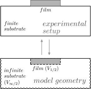
Figure 1: Comparison of the model geometry with the schematic experimental setup. In the model, film and substrate are of the same material so as to be able to use Eq. (5).

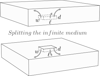
Figure 2: The model and its mirror image. Heat flow (arrows) does not cross the interface between model and image.

Our next simplification is to assume that the heating rate in the film does not depend on position, but only on time: $\dot{Q}\equiv\dot{Q}\left(t\right)$. Since the heating of the films we are considering will be caused by electrical current, this assumption is equivalent to assuming that the current density is uniform throughout the film. Explicit support for this comes from the work of Herrmann et al.,Herrmann98 ; Herrmann99 who found that in high-T_c tapes current in excess of a certain characteristic cutoff (the value of which was slightly below the critical current) was indeed distributed homogeneously across the entire superconductor cross section. Moreover, direct measurements on a slab of Bi-based crystal, using a microarray of Hall probes, show that although current is restricted to the lateral regions of the slab at relatively low temperature ($T\lesssim 50$ K), nonuniformity becomes negligible above about 80 K, a temperature relatively near $T_{c}$.Fuchs98 Again, a recent studyBobyl02 of YBa₂Cu₃O_7-δ strips using magneto-optical imaging found that even at so low a temperature as 20 K the nonuniformity of $J$ is only of the order of 20% when the transport current is 90% of its critical value. Finally, a uniform distribution of current throughout the cross section is the simplest explanation of the observation that critical current is independent of bridge width.Kunchur00 ; Ruibal07 ; Hahn95 ; Dinner07

Given uniform heating and the homogeneity of film and substrate (and since no measurements of local temperatures have yet been made on standard high-$T_{c}$ bridges), we are interested only in the volume-averaged temperature of the film. From Eq. (5),

$$T(t)=T_{b}+\frac{1}{V}\int_{\mathcal{V}}\int_{\mathcal{V}}\int_{0}^{t}\frac{\dot{Q}(t_{0})}{4\pi\kappa}T_{G}(\vec{r},t|\vec{r}_{0},t_{0})\;\mathrm{d}t\;\mathrm{d}^{3}\vec{r}_{0}\;\mathrm{d}^{3}\vec{r}$$

$$=T_{b}+\int_{\mathcal{V}}\int_{0}^{t}\frac{\dot{Q}(t_{0})}{4\pi\kappa}\times\Bigl{[}\frac{\sqrt{\pi}\lambda}{4d}\left(\mathrm{erf}\,\frac{d-\eta}{\lambda}+\mathrm{erf}\,\frac{d+\eta}{\lambda}\right)\times$$

$$\,\,\,\,\,\,\,\,\,\,\,\,\,\,\,\,\,\times\frac{\sqrt{\pi}\lambda}{2w}\left(\mathrm{erf}\,\frac{w/2-\xi}{\lambda}+\mathrm{erf}\,\frac{w/2+\xi}{\lambda}\right)\times$$

$$\,\,\,\,\,\,\,\,\,\,\,\,\,\,\,\,\,\times\frac{\sqrt{\pi}\lambda}{2\ell}\left(\mathrm{erf}\,\frac{\ell/2-\zeta}{\lambda}+\mathrm{erf}\,\frac{\ell/2+\zeta}{\lambda}\right)\Bigr{]}\;\mathrm{d}t_{0}\,\;\mathrm{d}\vec{r}_{0}$$

$$=T_{b}+\int_{0}^{t}\frac{\dot{Q}(t_{0})}{c}\,M(t-t_{0})\;\mathrm{d}t_{0}$$ (6)

where $V$ is the volume of $\mathcal{V}$, $\lambda=2\sqrt{D(t-t_{0})}$ is the diffusion length, erf is the error function, and

$$M(t-t_{0})=[\mathrm{erf}\,\frac{w}{\lambda}+\frac{\lambda}{\sqrt{\pi}w}(e^{-\frac{w^{2}}{\lambda^{2}}}-1)]\times$$

$$\,\,\,\,\,\,\,\,\,\,\,\,\,\,\times[\mathrm{erf}\,\frac{\ell}{\lambda}+\frac{\lambda}{\sqrt{\pi}\ell}(e^{-\frac{\ell^{2}}{\lambda^{2}}}-1)]\times$$

$$\,\,\,\,\,\,\,\,\,\,\,\,\,\,\times[\mathrm{erf}\,\frac{2d}{\lambda}+\frac{\lambda}{\sqrt{\pi}2d}(e^{-\frac{4d^{2}}{\lambda^{2}}}-1)]$$ (7)

Note that although the precise shape of the transfer functionRabiner75 Born75 $M$ depends on the dimensions and diffusivity of the film, its general shape is as shown (reversed) in Fig. 3. This means that in the final expression in Eq. (6), the convolutionOran88 of $\dot{Q}(t_{0})$ with $M(t-t_{0})$ gives considerably more weight to the immediate past and the present moment ($\underset{t_{0}\rightarrow t}{\lim}M(t-t_{0})=1$) than to the remote past ($\underset{t_{0}\rightarrow-\infty}{\lim}M(t-t_{0})=0$) - as in fact was only to be expected. We exploit this behaviour by making a further approximation consisting in the replacement of $M$ as defined in Eq. (7) by $M_{\tau}$, a rectangular function of unit height that is non-zero on the interval $[0,\tau]$, where $\tau$ is the area under $M$ (Fig. 4):

$$T(t)=T_{b}+\int_{0}^{t}\frac{\dot{Q}(t_{0})}{c}\,M_{\tau}(t-t_{0})\;\mathrm{d}t_{0}=T_{b}+\int_{t-\tau}^{t}\frac{\dot{Q}(t_{0})}{c}\;\mathrm{d}t_{0}$$ (8)

Figure 3: Schematic diagrams of the heating rate $\dot{Q(t_{0})}$ and the transfer function $M(t-t_{0})$ at two times, $t$ and $t^{\prime}>t$.

Figure 4: Comparison of the transfer function $M(t-t_{0})$ with its approximation, $M_{\tau}(t-t_{0})$.

We call $\tau$ the characteristic time of the film. Furthermore, since $M_{\tau}$ clearly overweights the proximal past, we slightly correct the integral by taking $\dot{Q}(t_{0})$ to have the value $\dot{Q}(t-\tau)$ for all $t_{0}$ in $[t-\tau,t]$, i.e. we replace $M_{\tau}(t-t_{0})$ with $M_{\delta}=\tau\delta(t-\tau-t_{0})$. Thus, finally (insofar as the dependence of temperature on time via the heating rate), $T(t)=\tau\dot{Q}(t-\tau)/c+T_{b}$, or

$$T(t+\tau)=\tau\frac{\dot{Q}[J,E(J,T(t))]}{c}+T_{b}$$ (9)

where the origin of the time-dependence of $\dot{Q}$ is explicitly displayed as the temperature- (and hence time-) dependence of $E(J)$, the intrinsic current-voltage characteristic (CVC) of the film.

Because of the structure of $M$ as a product of factors that each depend on only one spatial dimension (as well as on time, through $\lambda$), $\tau$ tends to zero whenever $w$, $l$ or $d$ do and the others are held fixed, and tends to the product of the other two factors whenever $w$, $l$ or $d$ tend to infinity; the larger $w$, $l$ and $d$, the larger is $\tau$, i.e. the greater the thermal inertia of the film, though $\tau$ always lies in [0,1]. That for a fixed thickness and width/length ratio the thermal behaviour of the film does depend on width, but increasingly less as width increases, has recently been confirmed experimentally.Ruibal07 The dependence of $\tau=\int_{0}^{\infty}M(t^{\prime})\;\mathrm{d}t^{\prime}$ on film width and length for a typical thickness (0.15 $\mathrm{\mu m}$) is shown as a contour map in Fig. 5.

Figure 5: Isolines of the characteristic time $\tau$ of a typical film 0.15 $\mathrm{\mu m}$ thick as a function of film width and length.

Note that if with a fixed current density $J$, $T$ tends to a stable value $T_{\infty}$, then Eq. (9) is asymptotically equivalent to Eq. (8), because $\dot{Q}$ must then also be stable and can therefore be taken out from under the integral in Eq. (8).

Since our heat source is in this study the Joule effect of a constant current, the form of $\dot{Q}[J,E(J,T)]$ in Eq. (9) is

$$\dot{Q}[J,E(J,T)]=JE(J,T)$$ (10)

For $E(J,T)$, which is not known (the experimental CVCs at constant bath temperature showing the very distortion that is investigated in this study), we shall use two empirical functions with different forms in order to show that our results do not depend critically on this aspect of the model. The first, variants of which have been used in previous work by ourselvesVinha03 ; Maza08 and others,Solovjov94 ; Fisher85 ; Prester98 is

$$E_{n}(J,T)=E_{0}(T)\,\big{[}\frac{J}{J_{0}(T)}-1\big{]}^{n}$$ (11)

where $E_{0}(T)=E_{01}(1-T/T_{c})^{m}$ and $J_{0}(T)=J_{01}(1-T/T_{c})^{m}$. The second is

$$E_{s}(J,T)=\rho_{n}(T)\,\big{[}J^{\frac{1}{s}}-J_{0}(T)^{\frac{1}{s}}\big{]}^{s}$$ (12)

where $J_{0}(T)$ is as in Eq. (11), $s=s_{0}+s_{1}(1-T/T_{c})$, and $\rho_{n}(T)$ is obtained by extrapolation from data for the temperature dependence of the resistivity of the normal (non-superconducting) film. Both have four adjustable parameters ($E_{01},\,J_{01},\,m\,\mathrm{and}\,n$ in Eq. (11), $J_{01},\,m,\,s_{0}\,\mathrm{and}\,s_{1}$ in Eq. (12) and, as in previous work, both are to be fitted to experimental $(J,E)$ data for the region of small $E$, where little heat is generated and the experimental CVC can accordingly be expected to lie close to the intrinsic CVC. We shall call the isotherms corresponding to $E_{n}$ and $E_{s}$, n-isotherms and s-isotherms, respectively. It may be noted that whereas $E_{s}$ tends to the natural limit $\rho_{n}J$ when $J\gg J_{0}$ or $T\longrightarrow T_{c}$, this is not so for $E_{n}$.

III.2 Parameterizing and testing the model

The films whose thermal behaviour we used to test the model and its predictions were two YBa₂Cu₃O_7-δ bridges on SrTiO${}_{\text{3}}$ substrates. One (sample mA) was a $50\times 10\times 0.12\,\mu\textrm{m}$ film with $T_{c}$=89.8 K, $\rho_{n}$(100 K) = 117 $\mu\Omega$cm and $\rho_{n}$(300 K) = 374 $\mu\Omega$cm; other features have been published elsewhere.Vinha03 The other (sample m50a) was longer and wider ($500\times 50\times 0.12\,\mu\mathrm{m}$), with $T_{c}$=87.1 K, $\rho_{n}$(100 K) = 190 $\mu\Omega$cm, and $\rho_{n}$(300 K) = 490 $\mu\Omega$cm.Ruibal07 By way of illustration, Fig. 6 shows the s-isotherms fitted by least squares to experimental $(J,E)$ data for sample m50a.

The diffusivity $D$ of the superconducting bridge material is $0.05\,\mathrm{cm^{2}/s}$, and that of the SrTiO${}_{\text{3}}$ substrate $0.18\,\mathrm{cm^{2}/s}$.Touloukian70 The intermediate value to be used in the model (see the second paragraph of the previous section) was informally optimized to afford adequate fit between the experimental values of $J^{*}(T_{b})$ for sample m50A and predicted values that were obtained as follows.

Although $J^{*}(T_{b})$ is defined as the current density at which a voltage jump occurs, Eqs. (9)-(12) show that this voltage jump will be accompanied by a temperature jump. Thus $J^{*}(T_{b})$ may be predicted by using these equations to simulate an experimental plot of temperature against current until a discontinuity occurs. Starting at a bath temperature $T_{b}$ at time 0, the temperature $T(\tau)$ attained after applying a current density $J_{c}+\delta J$ for time $\tau\ll\delta t$ is given by Eqs. (9), (10) and either (11) or (12) (where $\delta J$ is the current density step used in the experiments, typically 0.05 $\mathrm{MA}/\mathrm{cm^{2}}$, and $\delta t$ the step length, typically 1 ms); $T(2\tau)$ is similarly obtained using $T(\tau)$ as starting temperature; and so on until the total time elapsed is $\delta t$, whereupon the current density is increased by $\delta J$, etc. The current density at which a sudden temperature jump is observed is identified as $J^{*}(T_{b})$.

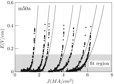
Figure 6: Large dots show experimental current-voltage characteristics (CVCs) of a 50$\mu$m-wide YBa₂Cu₃O_7-δ film at bath temperatures $T_{b}$ of (from right to left) 72.1, 73.5, 76.5, 78.0, 81.2, 82.3 and 84.2 K. Vertical dotted lines indicate voltage jumps at $J^{*}(T_{b})$. Continuous curves show s-isotherms [Eq. (12)] fitted to the data with E values in the shaded region.

Fig. 7 shows plots of $(T-T_{b})$ against $J$ obtained in this way using s-isotherms, and Table 1 confirms good fit between the predicted values of $J^{*}$ (and those predicted similarly using n-isotherms) and the experimental values. The achievement of such good fit with such a crude model is possibly attributable partly to the fact that for each $T_{b}$ the value of $J^{*}(T_{b})$ lies only about 20% above the largest $J$ in the set of $(J,E)$ data to which Eqs. (11) and (12) were fitted, i.e. extrapolation was quite limited; partly to the temperature and voltage jump occurring only 1-3 K above $T_{b}$ (see Fig. 7), i.e. far from $T_{c}$; and, given these circumstances, to the above-noted equivalence of Eqs. (9) and (8) for $\tau\ll\delta t$ and $J_{c}<J<J^{*}$.

The value of $D$ affording the above results was 0.12 $\mathrm{cm^{2}}/\mathrm{s}$; that this is closer to the diffusivity of the subtrate than to that of the superconductor seems reasonable, since the thermal diffusion length of the substrate for a time of 1 ms is rather more than 250 $\mu\mathrm{m}$, which is much larger than the film. The same value of $D$ also performed well for sample mA. The corresponding values of $\tau$ are 0.15 $\mu\mathrm{s}$ for film mA and 0.55 $\mu\mathrm{s}$ for m50A; as required by the above algorithm, these values are both much shorter than the experimental step length, 1 ms. Note that according to Eq. (9) the characteristic time $\tau$ is the time taken by the film to return to the bath temperature $T_{b}$ when heating is stopped. Accordingly, the use of current pulses lasting just a few tenths of a microsecondHarrabi09 and separated by intervals of similar length should allow the measurement of current-voltage curves that are nearly free from artifactual thermal effects.

Figure 7: Excess temperature of sample m50A, relative to the bath temperature $T_{b}$, as calculated using Eq. (9) and $s$-isotherms [Eq. (12)] in simulations in which the current density $J$ was increased by 0.05 $\mathrm{MA}/\mathrm{cm^{2}}$ at 1 ms intervals. From right to left, $T_{b}=$ 72.1, 73.5, 76.5, 78.0, 81.2, 82.3 and 84.2 K. A temperature jump occurs 1-3 K above the bath temperature, the excess temperature decreasing with increasing $T_{b}$.

Table 1: Experimentally observed supercritical currents of sample m50a at seven bath temperatures, together with the values obtained in simulations of experimental runs using Eq. (9) and either $n$-isotherms [$J_{n}^{*}$; Eq. (11) or $s$-isotherms $J_{s}^{*}$; Eq. (12)].

$T_{b}(K)$	$J_{exp}^{*}\,(\frac{MA}{cm^{2}})$	$J_{n}^{*}\,(\frac{MA}{cm^{2}})$	$J_{s}^{*}\,(\frac{MA}{cm^{2}})$
72.1	6.27	6.50	6.50
73.5	5.86	5.95	5.95
76.5	4.84	4.80	4.80
78.0	4.04	4.20	4.25
81.2	2.82	2.90	2.95
82.3	2.49	2.40	2.50
84.2	1.61	1.55	1.65

IV Stability

Eq. (9) is a nonlinear autonomous difference equation of first order.Elaydi99 To examine the stability of $T$ at constant $T_{b}$ and under a fixed current density $J$ we rewrite this equation in the form

$$T(t+\tau)=\mathcal{T}_{Q}[T(t);J]$$ (13)

where $\mathcal{T}_{Q}[T(t);J]\equiv\tau\,\frac{{Q}[T(t),J]}{c}+T_{b}$, and we note that under the given conditions $\mathcal{T}_{Q}(T;J)$ is convex and monotonically increasing, and that $\mathcal{T}_{Q}(T_{b};J)>T_{b}$ (since the current must heat the film). The condition for attainment of a stable temperature $T_{\infty}$ is that the graph of $\mathcal{T}_{Q}(T;J)$ intersect the line $T(t+\tau)=T(t)$, as may be seen by examining the staircase diagramElaydi99 shown in Fig. 8, in which vertical arrowed lines indicate real changes in temperature during a time increment $\tau$, while horizontal lines translate the final temperature of one $\tau$-interval into the starting temperature of the next. Not only does the path $0\rightarrow 1\rightarrow 2\rightarrow 3\rightarrow\cdots$ lead from its starting point ($T_{b}$) to the limiting temperature $T_{\infty}$ (a fixed point of $\mathcal{T}_{Q}(T;J)$), but so does the path $1^{*}\rightarrow 2^{*}\rightarrow 3^{*}\rightarrow\cdots$, i.e. any fluctuation to a temperature higher than $T_{\infty}$ will be recovered from. By contrast, if $\mathcal{T}_{Q}(T;J)$ meets the line $T(t+\tau)=T(t)$ tangentially the limiting temperature $T^{*}$ is not stable (Fig. 9), and if $\mathcal{T}_{Q}(T;J)$ lies wholly above $T(t+\tau)=T(t)$ there is no limiting temperature (Fig. 10).

Figure 8: Staircase diagram of thermal dynamics under an electrical current density $J<J^{*}$. The inset shows, as a function of time, the approach to the stable limiting temperature $T_{\infty}$ from below.

Figure 9: Staircase diagram of thermal dynamics under an electrical current density $J=J^{*}$. Starting at low values, temperature increases towards the asymptotically limiting value $T^{*}$, but this limit is unstable: starting from higher values, temperature increases indefinitely.

Figure 10: Staircase diagram of thermal dynamics under an electrical current density $J>J^{*}$. The rate of increase of temperature slows down, but finally increases without limit.

It may be enlightening to compare the above situations with that of a normal conductor, for which $E(T,J)=\rho(T)J$, where the electrical resistivity $\rho(T)=\rho_{0}+\rho_{1}T$. $\mathcal{T}_{Q}(T;J)$ is in this case a linear function of temperature, and whether it intersects the line $T(t+\tau)=T(t)$ (i.e. whether a stable limiting temperature is attained) therefore depends on the slope of this linear function. For copper, for example, $\partial\mathcal{T}_{Q}/\partial T\lesssim 10^{-3}$ for $J=1$ MA/cm² and $\tau=0.14$ $\mu$s,Buch99 so the absence of thermal runaway is ensured.

Since $\mathcal{T}_{Q}(T,J)$ increases with $J$ [by Eq. (10)], increasing the current density with a given bath temperature results in the location of the curve $\mathcal{T}_{Q}(T;J)$ progressing from that shown in Fig. 8 to that shown in Fig. 10; and examination of the definition of $\mathcal{T}_{Q}(T;J)$ shows that the greater the thermal inertia of the superconducting film (i.e. the greater $\tau$), the smaller the current at which instability sets in. The supercritical current density $J^{*}$ is the current density corresponding to Fig. 9, a situation that can be characterized by the conditions

$$T^{*}=\mathcal{T}_{Q}(T^{*};J^{*})$$

$$\frac{\partial\mathcal{T}_{Q}}{\partial T}(T^{*};J)=1$$ (14)

Alternatively, $J^{*}$ can be characterized as the smallest current density such that:

$$\mathcal{T}_{Q}(T;J)\geq T,\quad\forall\;T>T_{b}$$ (15)

(and the supercritical temperature $T^{*}$ as the temperature at which equality holds), or as the largest current density for which the equation

$$\mathcal{T}_{Q}(T;J)\,=\,T$$ (16)

has a solution.

To ensure the identification of $J^{*}$ for a given $T_{b}$, we first find the solution $T_{\infty}$ of Eq. (16) for a value of $J$ just slightly greater than $J_{c}$, then for a slightly larger $J$, and so on, until the largest $J$ for which there is a solution is identified. This procedure is not a simulation analogous to those of Section 3, for example, because the criterion for increasing $J$ is not the time elapsed but the satisfaction of a criterion of convergence that cannot be verified experimentally (at least at present). In experimental practice and simulations, $J$ is not kept fixed indefinitely; if $J$ is increased too fast, $J^{*}$ will be missed, though the thermal runaway will of course occur (alternatively, if $\mathcal{T}_{Q}(T;J)$ approaches $T(t+\tau)=T(t)$ quite closely in the situation of Fig. 10, the slowing down of the increase in temperature may be erroneously taken to indicate approach to a non-existent $T_{\infty}$).

For the films considered in Section 3, Fig. 11 shows the good fit between the $J^{*}(T_{b})$ functions obtained as above and the experimental data. Experimental error may reasonably be regarded as negligible (at least at this representation scale), because the current at which the voltage jump takes place is quite well defined, the current-voltage curve being locally nearly vertical. That $J^{*}(T_{b})$ lies at higher values for sample mA than for m50A is expected because of its smaller characteristic time and correspondingly lower $\mathcal{T}_{Q}(T;J)$.

Figure 11: Predictions of $J^{*}$ for samples mA and m50A obtained using Eq. (9), $s$-isotherms [Eq. (12)] and the convergence illustrated in Fig. 8 for $J$ values that were successively increased until convergence failed. The experimental points correspond to the abrupt voltage jumps observed in experimental CVCs (for sample m50A, Fig. 6).

Intuitively, the plots for mA and m50A in Fig. 11 differ because, the narrower the strip of film, the greater the proportion of it that is effectively cooled via its edges as well as via its bottom surface. It is therefore also to be expected that this edge effect will only be significant for film strips narrower than a few diffusion lengths. That this is so is indeed suggested by Fig. 12, which shows the surface $J^{*}(T_{b},\tau)$ calculated using $n$-isotherms for sample mA. For this superconductor and film thickness, only films with characteristic times below about 0.05 $\mu$s seem likely to be almost free from thermal instability. More generally, it appears that other mechanisms that limit superconductivity, such as the Larkin-Ovchinnikov electrodynamic instability, should be studied using films with very low $\tau$ (and/or very short intermittent current pulses, as mentioned above) if the effect being studied is not to be overwhelmed by the effect of thermal instability.

Figure 12: $J^{*}$ as a function of bath temperature $T_{b}$ and the characteristic time of the film, $\tau$.

V CONCLUDING REMARKS

This paper has developed a very simple analytical model in which strips of superconducting film supported by a substrate in a bath thermostatted at temperature $T_{b}$ are represented as rectangular blocks embedded in the surface of a semi-infinite medium of the same homogeneous material as the block. Assuming a uniform current density in the block, and given experimental current-voltage characteristics that allow parameterization of the model, the space-averaged thermal dynamics of the film prove to depend on its geometry through a single parameter, its characteristic time $\tau$. The quantitative predictions of the theory as regards the supercritical current density $J^{*}(T_{b})$ agree quite satisfactorily with experimental observations (Fig. 11).

Though in this paper the model has been parameterized for and tested on YBCO films 0.12$\,\mu\textrm{m}$ thick, its derivation involves nothing that prevents its application to other high-T_c or low-T_c films, so long as they do not require refrigeration with superfluid helium, the effective thermal conductivity of which is much greater than that of any ceramic substrateWilks87 even for boiling films.Maza89 Whether or not the good performance shown in Fig. 11 also generalizes to other films naturally remains to be seen. However, the mutual similarity of the current-voltage characteristics of all high-T_c superconductors suggests that they all become thermally unstable under high enough current densities, and that, with appropriate parameterization, our model should be able to predict this behaviour, thus explaining it in terms of thermal instability.

One of the key assumptions of the model is the homogeneity of the superconducting film, which together with the homogeneity of current density guarantees that the film and its behaviour are completely described by its geometry and current-voltage characteristics. Since YBCO films can have various degrees of inhomogeneity (mostly in relation to their oxygen content),Qadri97 the successful application of the model to mA and m50A suggests that the inhomogeneity of these samples, if any, was sufficiently finely grained as to be negligible. Further investigation of this issue probably requires examination of numerous individual cases; certainly, it seems safe to suppose that inhomogeneities can only accelerate thermal runaway.

In this paper the intrinsic current-voltage characteristics of the film, which are required for calculation of its heating rate [Eq. (10)], have been approximated by extrapolation from the low-energy region of the experimental CVCs. Although the experimental CVCs suffer from the very inaccuracies, the possible thermal origin of which is being investigated, it is assumed that their low-energy regions coincide sufficiently closely with the required intrinsic CVCs. That the functional form used for extrapolation is not excessively critical is supported in Table 1 by the agreement between $J_{n}^{*}$ and $J_{s}^{*}$ and the agreement of both with $J_{exp}^{*}$. Extrapolation will not be necessary if ultra-fast current-voltage measurements with nanosecond-scale measuring times become available, since such measurements may be expected, for the reasons explained above, to be devoid of thermal distortion.

The most disconcerting feature of our model is no doubt its treating the superconducting film and the substrate as a single continuum, with a single diffusivity coefficient (the sole free parameter of the model) and no acoustic mismatch between film and substrate. However, the value of the diffusivity coefficient seems not to be excessively critical (a single value worked well at all bath temperatures for both the samples considered here); while the lack of acoustic mismatch means that our results support the significance of thermal instability effects even under the conditions that are least conducive to such effects, i.e. with optimal thermal coupling between film and substrate. Numerous authors have acknowledged the determinant role of thermal effects when thermal impedance is high, but have implicitly or explicitly denied that they are significant when thermal coupling is good.

To sum up, in previous studies, finite element calculationsMaza08 have predicted the occurrence of a thermally driven transition to the normal conductance state at zero applied magnetic field when a homogeneous superconducting film is subjected to a controlled electrical current exceeding a certain “supercritical” value that coincides with experimental observations.

The present work supports those findings analytically. Experimental research on the breakdown of superconductivity due to other mechanisms (Larkin-Ovchinnikov vortex instabilities, hot spots, phase-slip centres) must accordingly be carried out under conditions that exclude the possibility of the heat-driven transition, and vice versa.

VI Acknowledgements

We gratefully acknowledge support by the Spanish Ministry of Science and Innovation through contract ERDF FIS2010-19807 and by the Xunta de Galicia through ERDF 2010/XA043 and 10TMT206012PR.

Our special appreciation to Ian Coleman from the University of Santiago de Compostela for his decisive role in the English restyling of this paper.

References

- [1] S. G. Doettinger, R. P. Huebener, R. Gerdemann, A. Kühle, S. Anders, T. G. Träuble, and J. C. Villégier. Electronic instability at high flux-flow velocities in high- superconducting films. Phys. Rev. Lett., 73(12):1691–1694, Sep 1994.
- [2] M. N. Kunchur. Unstable flux flow due to heated electrons in superconducting films. Phys. Rev. Lett., 89:137005–4, 2002.
- [3] D. Babić, J. Bentner, C. Sürgers, and C. Strunk. Flux-flow instabilities in amorphous Nb0.7Ge0.3 microbridges. Phys. Rev. B, 69(9):092510, Mar 2004.
- [4] E.V. Bezuglyi and I.V. Zolochevskii. Phase diagram of a current-carrying superconducting film in absence of the magnetic field. Low Temp. Phys., 36:1008, 2010.
- [5] P. Bernstein, J.F. Hamet, M.T. González, and M. Ruibal. Vortex dynamics at the transition to the normal state in YBa2Cu3O7-δ films. Physica C, 455:1–12, 2007.
- [6] M. Lindmayer and M. Schubert. IEEE Trans. on Appl. Supercond., 3:884, 1993.
- [7] T. Kiss, M. Inoue, K. Hasegawa, K. Ogata, V.S. Vysotsky, Yu. Ilyin, M. Takeo, H. Okanoto, and F. Irie. Quench characteristics in htsc devices. IEEE Trans. on Appl. Supercond., 9:1073–1076, 1999.
- [8] A. Lehner, A. Heinrich, K. Numssen, and H. Kinder. Probing the temperature during switching of YBCO films. Physica C, 372:1619–1621, 2002.
- [9] Transition to the normal state induced by high current densities in YBa2Cu3O7-δ.
- [10] A. Vl. Gurevich and R. G. Mints. Self-heating in normal metals and superconductors. Rev. Mod. Phys., 59(4):941–999, Oct 1987.
- [11] P. M. Morse and Feshback H. Methods of Theoretical Physics. McGraw-Hill Co., New York, USA, 1953.
- [12] G. Barton. Elements of Green’s Functions and Propagation. Clarendon-Press, Oxford, 1995.
- [13] Adrian Bejan and Allan D. Kraus, editors. Heat transfer handbook. John Wiley & Sons, 2003.
- [14] M. Nahum, S. Verghese, P.L. Richards, and K. Char. Thermal boundary resistance for YBa2Cu3O7-δ films. Appl. Phys. Lett., 59:2034–2036, 1991.
- [15] C.D. Marshall, A. Tokmakoff, I.M. Fishman, C.B. Eom, Julia M. Phillips, and M.D. Fayer. Thermal boundary resistance and diffusivity measurements on thin YBa2Cu3O7-δ films with MgO and SrTiO3 substrates using the transient grating method. J. Appl. Phys., 73:850–857, 1993.
- [16] Bincheng Li, L. Pottier, J.P. Roger, and D. Fournier. Thermal characterization of thin superconducting films by modulated thermoreflectance microscopy. Thin Solid Films, 352:91–96, 1999.
- [17] J. Herrmann, N. Savvides, K.H. Mller, R. Zhao, G. McCaughey, F. Dermann, and M. Apperley. Current distribution and critical current state in superconducting silver-sheathed (bi-pb)-2223 tapes. Physica C, 305:114–124, 1998.
- [18] J. Herrmann, N. Savvides, K.H. Müller, R. Zhao, G.D. McCaughey, F.A. Darmann, and M.H. Apperley. Transport current distribution in (Bi,Pb)-2223/Ag tapes. IEEE Trans. Appl. Supercond., 9:1824–1827, 1999.
- [19] Dan T. Fuchs, E. Zeldov, M. Rappaport, T. Tamegai, S. Ooi, and H. Shtrikman. Transport properties governed by surface barriers in Bi2Sr2CaCu2O8. Nature, 391:373–376, 1998.
- [20] A.V. Bobyl, D.V. Shantsev, Y.M. Galperin, T.H. Johansen, M. Baziljevich, and S.F. Karmanenko. Relaxation of transport current distribution in a YBaCuO strip studied by magneto-optical imaging. Supercond. Sci. Technol., 15:82–89, 2002.
- [21] M.N. Kunchur, B.I. Ivlev, D.K. Christen, and J.M. Phillips. Metallic normal state of YBa2Cu3O7-δ. Phys. Rev. Lett., 84:5204–5207, 2000.
- [22] M. Ruibal, G. Ferro, M. R. Osorio, J. Maza, J. A. Veira, and F. Vidal. Size effects on the quenching to the normal state of YBa2Cu3O7-δ thin-film superconductors. Phys. Rev. B, 75(1):012504, Jan 2007.
- [23] R. Hahn, G. Fotheringham, and J. Klockau. Critical current dependency on line width and long term stability of epitaxial YBa2Cu3O7-δ thin films lines. IEEE Trans. Appl. Supercond., 5:1440–1443, 1995.
- [24] Rafael B. Dinner, Kathryn A. Moler, D. Matthew Feldmannn, and M.R. Beasley. Imaging ac losses in superconducting films via scanning hall probe microscopy. Phys. Rev. B, 75:144503–12, 2007.
- [25] Laurence R. Rabiner and Bernard Gold. Theory and applications of digital signal processing. Prentice-Hall, New Jersey, 1975.
- [26] Max Born and Emil Wolf. Principles of Optics. Pergamon Press, Oxford, 1975.
- [27] E. Oran Brigham. The Fast Fourier transform and its applications. Prentice-Hall, New Jersey, 1988.
- [28] J. Via, M. T. González, M. Ruibal, S. R. Currás, J. A. Veira, J. Maza, and F. Vidal. Self-heating effects on the transition to a highly dissipative state at high current density in superconducting YBa2Cu3O7-δ thin films. Phys. Rev. B, 68:224506–10, 2003.
- [29] V. F. Solovjov, V. M. Pan, and H. C. Freyhardt. Anisotropic flux dynamics in single-crystalline and melt-textured YBa2Cu3O7-δ. Phys. Rev. B, 50:13724–13734, 1994.
- [30] D. S. Fisher. Sliding charge-density waves as a dynamic critical phenomenom. Phys. Rev. B, 31:1396–1427, 1985.
- [31] M. Prester. Current transfer and initial dissipation in high-Tc superconductors. Supercond. Sci. Technol., 11:333–357, 1998.
- [32] Y.S. Touloukian, editor. Thermophysical Properties of Matter, volume 2,5. Plenum Press, New York, 1970.
- [33] K. Harrabi, F.-R. Ladan, Vu Lam, J.-P. Maneval, J.-F. Hamet, J.-C. Villégier, and R. Bland. Current-temperature diagram of resistive states in long superconducting YBa2Cu3O7 strips. J. Low Temp. Phys., 157:36–56, 2009.
- [34] Saber N. Elaydi. An Introduction to Difference Equations. Springer-Verlag, New York, 1999.
- [35] A. Buch. Pure Metals Properties. ASM International, Ohio, USA, 1999.
- [36] J. Wilks and D.S. Betts. An Introduction to Liquid Helium. Clarendon Press, Oxford, 2nd. edition, 1987.
- [37] J. Maza, F. Jebali, M.X. François, and F. Vidal. Temperature and heat flux measurements in noiseless film boiling in superfluid helium with a flat heater. Cryogenics, 29(3):200 – 202, 1989.
- [38] S.B Qadri, E.F Skelton, P.R Broussard, V.C Cestone, M.S Osofsky, V.M Browning, M.E Reeves, and W Prusseit. Structural inhomogeneities in thin epitaxial films of YBa2Cu3O7-δ and their effects on superconducting properties. Thin Solid Films, 308-309:420 – 424, 1997.
- [39] When voltage instead of current is controlled the physics is quite different. Heat input no longer increases monotonically with voltage (which can lead to multivalued CVCs), and superconducting zones can coexist with normal zones (e.g. due to hot spots). These phenomena lie outside the scope of this paper.