Simulation of a moving liquid droplet inside a rarefied gas region

Abstract

We study the dynamics of a liquid droplet inside a gas over a large range of the Knudsen numbers. The moving liquid droplet is modeled by the incompressible Navier-Stokes equations, the surrounding rarefied gas by the Boltzmann equation. The interface boundary conditions between the gas and liquid phases are derived. The incompressible Navier-Stokes equations are solved by a meshfree Lagrangian particle method called Finite Pointset Method (FPM), and the Boltzmann equation by a DSMC type of particle method. To validiate the coupled solutions of the Boltzmann and the incompressible Navier-Stokes equations we have further solved the compressible and the incompressible Navier-Stokes equations in the gas and liquid phases, respectively. In the latter case both the compressible and the incompressible Navier-Stokes equations are also solved by the FPM. In the continuum regime the coupled solutions obtained from the Boltzmann and the incompressible Navier-Stokes equations match with the solutions obtained from the compressible and the incompressible Navier-Stokes equations. In this paper, we presented solutions in one-dimensional physical space.

1 Introduction

Gas-liquid flows in small scale geometries have received considerable attention in the past few years, especially due to the rapid developments in micro- and nanofluidics. Recently, experiments have been performed in which a segmented flow of gas and liquid is studied in nanochannels [KKH, OFdeBM, PNYJetal]. The Knudsen number of these flows, i.e. the ratio of the mean free path of the particles and the characteristic length, is such that the Boltzmann equation needs to be solved to describe the transport processes in the gas phase, while usually the incompressible Navier-Stokes equations are sufficient to model the liquid phase. While numerical methods for solving the Boltzmann equation are well established [Bird, NS95], no efficient methods seem to exist to study the flow of a gas at rarefied conditions coupled to the liquid flow described by the incompressible Navier-Stokes equations. The aim of this article is to take first steps into that direction.

We consider a liquid droplet inside a gas. A liquid droplet may move, for example, due to a pressure difference, so that we need to solve a moving interface problem. One may choose different methods to compute these types of two-phase flows with moving interface, however, meshfree Lagrangian particle methods seem to be one of the preferred choices for such problems. For the rarefied gas phase we solve the Boltzmann equation by a DSMC type of particle method [NS95, BI89]. In DSMC type of methods the gas particles are Lagrangian particles and move with their molecular velocities. However, these methods are mesh-based since one divides a computational domain into cells and performs intermolecular collisions of particles inside cells. Moreover, macroscopic quantities like fluid density, velocity, temperature, etc. are stored in the cell centers. On the other hand, we solve the incompressible Navier-Stokes equations by the Finite Pointset Method(FPM) [TK07, TKH09], which is a meshfree Lagrangian particle method and is similar in character as Smoothed Particle Hydrodynamics (SPH) [GM77]. Within the FPM we approximate a liquid domain by Lagrangian particles which move with the local fluid velocity. We note that in this article we utilize two types of particles which may confuse the readers. Therefore, we call the DSMC particles ”gas molecules” and the FPM particles ”gas- and liquid particles” for the gas- and liquid phases, respectively. FPM particles are numerical grid points that move with the fluid velocity and carry all fluid dynamic quantities like densities, velocities, pressures, etc. along with them. To solve this type of two-phase flow problem one has to decompose the computational domain into a liquid and a gas domain. The domain decomposition is performed by first generating the entire domain by regular cells which are DSMC cells. Then we generate liquid particles overlapping the DSMC cells. The interface between the two domains is determined from the liquid particles. In the one-dimensional case, it is easily determined by identifying the extreme ends of the liquid particle positions. For higher-dimensional problems the interface is determined by identifying the free surface particles among the liquid particles, see [TK02, TK07] for details.

To the best of the author’s knowledge, this is the first attempt to couple numerically the incompressible Navier-Stokes equations and the Boltzmann equation in the rarefied regime. To validate the coupled solution of the equations we have further simulated the gas and liquid phases by solving the compressible and the incompressible Navier-Stokes equations, respectively. In the latter case the interface conditions are quite standard which have been reported in a number of articles in the past few years [BKZ, HW, HN, KP, TK07], see also the references therein. We have considered the same examples as presented in [CFA00, FMO98], where the flow has been modeled by the Euler or the Navier-Stokes equations. Since we solve both the compressible and the incompressible equations by a particle method, we use different flags to distinguish the gas and liquid particles. Interfaces between the fluids can be determined based on their flags or colors [TK02, MORRIS]. The flags are defined initially, and particles carry them along and leave them unchanged during the simulations.

As will be shown in the article, for small Knudsen numbers the solutions obtained from the coupling of the Boltzmann and the incompressible Navier-Stokes equations are very close to the solutions obtained from the coupling of the compressible and the incompressible Navier-Stokes equations. However, the same is no longer true for the larger Knudsen numbers. We present test cases with smaller as well as larger Knudsen numbers.

The paper is organized as follows. In section 2, we introduce the mathematical model for the gas and the liquid phases. In addtion to that we derive the interface boundary conditions. In section 3, we describe the particle methods for solving the Boltzmann and the Navier-Stokes equations. Section 4 is devoted to the coupling algorithms for the gas and the liquid phases. The numerical tests are presented in section 5, and some concluding remarks are given in section 6.

2 Mathematical Model

2.1 Gas phase: the Boltzmann and the compressible Navier-Stokes equations

The Boltzmann equation describes the time evolution of a distribution function $f(t,{\bf x},{\bf v})$ for particles of velocity ${\bf v}\in{}^{3}$ at point ${\bf x}\in\Omega\subset{}^{s},(s=1,2,3)$ and time $t\in{}_{+}$. It is given in nondimensional form as

$${\frac{\partial f}{\partial t}}+{\bf v}\cdot\nabla_{x}f=\frac{1}{\epsilon}J(f,f),$$ (1)

where $\epsilon$ is the Knudsen number, $J(f,f)$ is the collision operator which is given for hard spheres by

$$J(f,f)=\int_{{}^{3}}\int_{S^{2}}\beta(|{\bf v}-{\bf w}|,{\bf n})[f({\bf v}^{{}^{\prime}})f({\bf w}^{{}^{\prime}})-f({\bf v})f({\bf w})]d{\bf n}d{\bf w},$$ (2)

where $S^{2}$ is the unit sphere in ³, ${\bf n}\in S^{2}$ is the unit vector in the impact direction, $\beta$ is the collision cross section, $f({\bf v}^{{}^{\prime}})=f(t,{\bf x},{\bf v}^{{}^{\prime}})$ and analogously for $f({\bf v})$ etc. The pairs $({\bf v},{\bf w})$ and $({\bf v}^{{}^{\prime}},{\bf w}^{{}^{\prime}})$ are the pre- and post collisional velocities of two colliding particles, given by

$${\bf v}^{{}^{\prime}}={\bf v}-{\bf n}\left[{\bf n}\cdot({\bf v}-{\bf w})\right],\quad{\bf w}^{{}^{\prime}}={\bf w}+{\bf n}\left[{\bf n}\cdot({\bf v}-{\bf w})\right].$$ (3)

The collision operator has five collisional invariants $\psi({\bf v})=1,{\bf v},|{\bf v}|^{2}/2$ satisfying

$$\int_{{}^{3}}\psi({\bf v})J(f,f)d{\bf v}=0.$$ (4)

In other words, $J(f,f)$ locally satisfies the conservation laws for mass, momentum and energy.

The basic quantities of interest are the macroscopic ones, like the density $\rho(t,{\bf x})$, mean velocity ${\bf u}={\bf u}(t,{\bf x})$ and the total energy $E=E(t,{\bf x})$, and are defined as

$$\rho=\int_{{}^{3}}f(t,{\bf x},{\bf v})d{\bf v},\quad\quad{\bf u}=\frac{1}{\rho}\int_{{}^{3}}{\bf v}f(t,{\bf x},{\bf v})d{\bf v}$$ (5)

$$E=\frac{1}{\rho}\int_{{}^{3}}\frac{|{\bf v}|^{2}}{2}f(t,{\bf x},{\bf v})d{\bf v}=\frac{1}{2}|{\bf u}|^{2}+e,$$ (6)

where $e$ is the internal energy, defined by

$$e=\frac{1}{\rho}\int_{{}^{3}}\frac{|{\bf v}-{\bf u}|^{2}}{2}f(t,{\bf x},{\bf v})d{\bf v}.$$ (7)

Moreover, the pressure tensor $\varphi$ and heat flux ${\bf q}$ are defined by

$$\varphi = \int_{{}^{3}}({\bf v}-{\bf u})\otimes({\bf v}-{\bf u})f(t,{\bf x},{\bf v})d{\bf v}$$ (8)

$${\bf q} = \int_{{}^{3}}\frac{|{\bf v}-{\bf u}|^{2}}{2}({\bf v}-{\bf u})f(t,{\bf x},{\bf v})d{\bf v}.$$ (9)

The gas pressure $p$ is defined as $p=\frac{2}{3}\rho e$ for a monoatomic ideal gas. Furthermore, $p=\rho RT$ holds, where $T$ is the temperature and $R$ is the gas constant. For more details we refer to [CIP94, Sone07].

Multiplying the Boltzmann equation by its collisional invariants and then integrating with respect to ${\bf v}$ over ³ we obtain the following local conservation equations

$$\frac{\partial\rho}{\partial t}+\nabla\cdot(\rho{\bf u}) = 0$$

$$\frac{\partial(\rho{\bf u})}{\partial t}+\nabla\cdot(\rho{\bf u}\otimes{\bf u}+\varphi) = 0$$ (10)

$$\frac{\partial(\rho E)}{\partial t}+\nabla\cdot\left[\rho E{\bf u}+\varphi\cdot{\bf u}+{\bf q}\right] = 0.$$

For $\epsilon$ tending to zero, i. e. for small mean free paths, one can show that the phase space distribution function $f$ tends to the local Maxwellian [Caf80]

$$f_{M}(t,{\bf x},{\bf v})=\frac{\rho}{(2\pi RT)^{3/2}}\;e^{-{\frac{|{\bf v}-{\bf u}|^{2}}{2RT}}}$$ (11)

and the system of moment equations (2.1) tends to the compressible Euler equations with the closure relations $\varphi=pI$ and ${\bf q}={\bf 0}$. This can be verified from the asymptotic expansion of $f$ in $\epsilon$, where the zeroth order approximation gives the local Maxwellian distribution, and the first order approximation [BGL] gives the Chapman-Enskog distribution

$$f_{CE}(t,{\bf x},{\bf v})=f_{M}(t,{\bf x},{\bf v})\left[1+\frac{2}{5}\frac{{\bf q}\cdot{\bf c}}{\rho(RT)^{2}}\left(\frac{|{\bf c}|^{2}}{2RT}-\frac{5}{2}\right)+\frac{1}{2}\frac{\tau:{\bf c}\otimes{\bf c}}{\rho(RT)^{2}}\right],$$ (12)

where ${\bf c}={\bf v}-{\bf u}$. At the same time, (2.1) tends to the compressible Navier-Stokes equations with the closure relations

$$\varphi=pI-\tau,\quad\quad{\bf q}=-\kappa\nabla T,$$ (13)

where

$$\tau_{ij}=\mu\left(\frac{\partial u_{i}}{\partial x_{j}}+\frac{\partial u_{j}}{\partial x_{i}}-\frac{2}{3}(\nabla\cdot{\bf u})~{}\delta_{ij}\right),$$ (14)

and $\mu=\mu(t,x)$ and $\kappa=\kappa(t,x)$ are the dynamic viscosity and thermal conductivity, respectively. They are of the order of $\epsilon$. For example, the first approximation for the viscosity and the thermal conductivity of a monatomic gas is given by [VK65]

$$\mu=\frac{5}{16d^{2}}\sqrt{\frac{mkT}{\pi}},\quad\quad\kappa=\frac{15k}{4m}\mu,$$ (15)

where $k$ is the Boltzmann constant, and $d$ and $m$ are the mass and the diameter of the molecules, respectively. In this paper we compute the parameters $\mu$ and $\kappa$ from the initial temperature, and use the corresponding values in the compressible Navier-Stokes equations.

Since we solve the Navier-Stokes equations with a meshfree Lagrangian particle method, we re-express them in Lagrangian form with respect to the primitive variables as

$$\frac{d{\bf x}_{g}}{dt} = {\bf u}_{g}$$

$${\frac{d\rho_{g}}{dt}} = -\rho_{g}\nabla\cdot{\bf u}_{g}$$

$${\frac{d{\bf u}_{g}}{dt}} = -\frac{1}{\rho_{g}}\nabla p_{g}+\nu_{g}\left[\nabla^{2}{\bf u}_{g}+\frac{1}{3}\nabla(\nabla\cdot{\bf u}_{g})\right]$$ (16)

$${\frac{dT_{g}}{dt}} = \frac{1}{c_{v}\rho_{g}}\left[-p_{g}~{}\nabla\cdot{\bf u}_{g}+(\tau_{g}\cdot\nabla)\cdot{\bf u}_{g}+{\kappa_{g}}\nabla^{2}T_{g}\right],$$

where we have used the index $g$ for the gas quantities, $\nu$ is the kinematic viscosity, $d/dt$ is the material derivative, $c_{v}$ is the specific heat at constant volume, given by $\frac{3}{2}R$ for a monoatomic gas. We note that we have expressed the internal energy of the gas as $e_{g}=c_{v}T_{g}$.

When introducing the specific heat into the energy equation an ideal gas was assumed. In addition to the system of equations (2.1) we consider the equation of state

$$p_{g}=\rho_{g}RT_{g}.$$ (17)

2.2 Liquid phase: Incompressible Navier-Stokes equations

We consider incompressible flow inside the liquid phase. The governing equations can be obtained from the incompressible Navier-Stokes equations by assuming the liquid density $\rho_{l}$ to be constant. All liquid quantities are denoted with the index $l$. Moreover, one can express the internal energy $e_{l}$ for the liquid phase approximately by $e_{l}=c_{p}T_{l}$, where $c_{p}$ is the specific heat at constant pressure [Lesieur]. We also solve the incompressible Navier-Stokes equations by a meshfree Lagrangian particle method. Therefore, we express these equations in Lagrangian form

$$\frac{d{\bf x}_{l}}{dt} = {\bf u}_{l}$$

$$\nabla\cdot{\bf u}_{l} = 0$$

$$\frac{d{\bf u}_{l}}{dt} = -\frac{\nabla p_{l}}{\rho_{l}}+\nu_{l}\nabla^{2}{\bf u_{l}}$$ (18)

$${\frac{dT_{l}}{dt}} = \frac{1}{c_{p}\rho_{l}}\left(\tau_{l}\cdot\nabla\right)\cdot{\bf u}_{l}+\frac{\kappa_{l}}{c_{p}\rho_{l}}\nabla^{2}T_{l},$$

where $\tau_{l}$ is given by (14) without the divergence of velocity term. In many situations, the viscous dissipation term in the energy equation can be neglected. A detailed discussion about when it is justified to omit that term can be found in [MS07, Morini05]. In what follows, we limit ourselves to scenarios with negligible viscous heating, resulting in a simplified energy equation

$$\frac{dT_{l}}{dt}=\frac{\kappa_{l}}{c_{p}\rho_{l}}\nabla^{2}T_{l}.$$ (19)

2.3 Initial and boundary conditions

In this paper we consider a one-dimensional computational domain $\Omega=[a,b]\subset{}^{1}$, where $a$ is always zero and $b$ varies from $10^{-4}$ to $10^{-6}$. The domain is initially decomposed into the gas domain $\Omega_{g}$ and liquid domain $\Omega_{l}=\Omega\setminus\Omega_{g}$. We consider cases where the liquid domain always remains inside of the full domain. Therefore, the boundaries $a$ and $b$ always belong to the gas domain. We prescribe boundary conditions for the gas at points $a$ and $b$. Moreover, there are interfaces between the liquid and the gas domains, and we have to further specify the interface boundary conditions, described in the next subsection.

In the gas domain $\Omega_{g}$ we either solve the compressible Navier-Stokes equations or the Boltzmann equation. We assume that initially the gas is in thermal equilibrium with the values $\rho_{g}(0,x),u_{g}(0,x)$ and $T_{g}(0,x)$, which are the initial conditions for the compressible Navier-Stokes equations. If we solve the Boltzmann equation in $\Omega_{g}$, we prescribe the initial condition as a local Maxwellian with parameters $\rho_{g}(0,x),{\bf u}_{g}(0,x)=(u_{g}(0,x),0,0)$ and $T_{g}(0,x)$. In $\Omega_{l}$ we solve the incompressible Navier-Stokes equations with initial conditions $p_{l}(0,x),u_{l}(0,x)$ and $T_{l}(0,x)$.

2.4 Interface boundary conditions

To couple the liquid and gas phases one has to first determine the interface between two phases and then prescribe the interface boundary conditions. For solving the Boltzmann and the incompressible Navier-Stokes equations, we determine the interface as the free surface particles from the liquid domain. In the one dimensional case, we have two interfaces, which are given by the liquid particle position at the extreme left $(x_{L})$ and the liquid particle position at the extreme right $(x_{R})$. They can be tracked at every time step. When we solve the transport equations in both phases by the FPM, we assign different flags or colors for the particles in the compressible and incompressible phases. The particles of each phase carry the color function along with them, and the interface can be tracked with the help of the flags of the particles. We again determine the interface by identifying the liquid particles at the extreme left and right.

Owing to the kinematic boundary condition at the interface, there is no penetration of particles from one phase to the other. This means that the convective terms for mass, momentum and energy transport are zero. Hence, all fluxes with the multiplicative factors ${\bf u}$ vanish. Therefore, we have the following jump conditions for the momentum and energy fluxes the system (2.1)

$$(\varphi_{11})_{l} = (\varphi_{11})_{g}$$ (20)

$$(\varphi_{11}u+q)_{l} = (\varphi_{11}u+q)_{g}.$$ (21)

Here we use a scalar quantity $q$ for the heat flux in the one-dimensional case. Moreover, we assume that the velocity and temperature at the interface are continuous, i.e.

$$u_{l}=u_{g}.$$ (22)

$$T_{l}=T_{g}.$$ (23)

Then from (20), (21) and (22) we have

$$q_{l}=q_{g}.$$ (24)

2.4.1 Interface boundary conditions for the compressible and the incompressible Navier-Stokes equations

We use the closure relations (13) and (14) in (20) and (24) and get the following continuity of the fluxes

$$\left(p-\frac{4}{3}\mu\frac{\partial u}{\partial x}\right)_{l} = \left(p-\frac{4}{3}\mu\frac{\partial u}{\partial x}\right)_{g}$$ (25)

$$\left(\kappa\frac{\partial T}{\partial x}\right)_{l} = \left(\kappa\frac{\partial T}{\partial x}\right)_{g}.$$ (26)

Using the divergence-free condition for the liquid we obtain the interface boundary condition for the pressure as

$$\left(p\right)_{l}=\left(p-\frac{4}{3}\mu\frac{\partial u}{\partial x}\right)_{g}.$$ (27)

We note that we use the condition (23) together with (26) for the thermodynamic equations.

2.4.2 Interface boundary conditions between the Boltzmann and the incompressible Navier-Stokes equations

An important point to note in relation to the interface conditions between the Boltzmann and the Navier-Stokes domain is the fact that while the quantities available on the gas side of the interface determine all of the quantities needed on the liquid side, the same is not true in the opposite direction. Therefore, additional assumptions have to be made when computing the interfacial phase-space distribution in the gas from the density, velocity and temperature in the liquid. This requires a different treatment depending on whether information is passed from the gas to the liquid or vice versa. As in the previous subsection 2.4.1 we assume the continuity of the velocity and the temperature as given by (22) and (23). In this case the closure relations (13) and (14) are used only for the fluxes of the incompressible Navier-Stokes equations. Therefore, the continuity relations for the fluxes differ and are re-expressed in the form

$$(p)_{l}=\left(\varphi_{11}\right)_{g}$$ (28)

$$-\left(\kappa\frac{\partial T}{\partial x}\right)_{l}=(q)_{g},$$ (29)

where $(\varphi_{11})_{g}$ and $(q)_{g}$ are computed directly from the moments (8) and (9), respectively, of the solution of the Boltzmann equation. Hence, (23), (28) and (29) give the interface conditions from the gas into the liquid, where $T_{g}$ is computed from the solution of the Boltzmann equation.

On the other hand, the interface boundary condition from the liquid into the gas is treated as follows. When gas molecules hit the interface, we apply the diffuse reflection condition with thermal accommodation, i.e. particles are reflected with the interface temperature and velocity into the gas domain, see the detailed descriptions in section 4.2.

3 Numerical methods

3.1 Particle method for the Boltzmann equation

For solving the Boltzmann equation we have used a variant of the DSMC method [Bird], developed in [NS95, BI89]. The method is based on the time splitting of the Boltzmann equation. Introducing fractional steps one first solves the free transport equation (the collisionless Boltzmann equation) for one time step. During the free flow, boundary and interface conditions are taken into account. In a second step (the collision step) the spatially homogenous Boltzmann equation without the transport term is solved. To solve the homogeneous Boltzmann equation the key point is to find an efficient particle approximation of the product distribution functions in the Boltzmann collision operator given only an approximation of the distribution function itself. To simulate this equation by a particle method an explicit Euler step is performed. To guarantee positivity of the distribution function during the collision step a restriction of the time step proportional to the Knudsen number is needed. That means that the method becomes exceedingly expensive for small Knudsen numbers.

3.2 FPM for the compressible Navier-Stokes equations

We solve the Navier-Stokes equations (2.1) by the FPM. As already pointed out, the FPM is a meshfree Lagrangian particle method, where we approximate the spatial derivatives with the help of the weighted least squares method. In order to solve these equations by FPM, one first fills the computational domain by particles which can be considered as moving numerical grid points and then approximates the spatial derivatives occurring on the right hand side of (2.1) at each particle position from its neighboring particles. This reduces the system of partial differential equations (2.1) to a system of ordinary differential equations with respect to time. We solve the resulting ODE system with the help of a two-step Runge-Kutta method. The time steps for the compressible as well as the incompressible Navier-Stokes equations are restricted by the CFL condition and by the value of the transport coefficient $max\left[\mu_{g}/\rho_{g},\kappa_{g}/(\rho_{g}c_{v}),\kappa_{l}/(\rho_{l}c_{p})\right]$. We refer to our earlier papers [TKH09, Tiw01] for the details of the least squares approximation of the spatial derivatives. We note that we need to introduce a particle management scheme during the simulations. Because of the Lagrangian description of the method particles may accumulate or may thin out causing holes in the computational domain. This gives rise to some instabilities of the method. Therefore, we have to add or remove particles. In the one-dimensional case this task is quite simple. If the distance between a particle and its nearest neighbor is larger than $1.2$ times the initial spacing of particles, we add a new particle in the center. On the other hand, if two particles are closer than $0.2$ times the initial spacing we remove both of them and add a new particle at the mid point. However, these adding and remove factors may depend upon users. The fluid dynamic quantities of newly added particles are approximated from their neighbor particles with the help of the least squares method.

3.3 FPM for the incompressible Navier-Stokes equations

The incompressible Navier-Stokes equations (2.2) are also solved by the FPM. Since we consider one-dimensional physical space, the solution of the incompressible Navier-Stokes equations is simple. For higher-dimensional physical spaces we refer to [TK02, TK07].

Taking the partial derivatives with respect to $x$ on both sides of the momentum equation (2.2) and using the divergence-free constraint, we obtain the one-dimensional Laplace equation for the pressure

$$\frac{\partial^{2}p_{l}}{\partial x^{2}}=0,$$ (30)

with the Dirichlet boundary conditions $p_{L}$ and $p_{R}$ on the left and right interfaces $x_{L}$ and $x_{R}$, respectively.

Suppose we have $N$ liquid particles ${x_{l1},\cdots,x_{lN}}$ in $\Omega_{l}$. We have to solve the corresponding transport equations for every liquid particle. Let $x_{li}$ be the position of an arbitrary particle. The new pressure at time level $t^{n+1}=(n+1)\Delta t$, where $\Delta t$ is the time step, can be computed explicitely by

$$p^{n+1}_{li}=\frac{p_{R}^{n}-p_{L}^{n}}{x_{R}^{n}-x_{L}^{n}}x_{li}^{n}+\frac{p_{R}^{n}x_{L}^{n}-p_{L}^{n}x_{R}^{n}}{x_{L}^{n}-x_{R}^{n}}.$$ (31)

The new velocity is given by

$$u^{n+1}_{li}=u^{n}_{li}-\frac{\Delta t}{\rho_{l}}(\frac{p_{R}^{n}-p_{L}^{n}}{x_{R}^{n}-x_{L}^{n}}).$$ (32)

The energy equation for the liquid is solved in the same way as in the case of the gas.

We note that the equation for the velocity does not contain any contributions from the viscous term, which is due to the one-dimensional nature of the problem. The thermal diffusivity $\kappa_{l}/(\rho_{l}c_{p})$ of the liquid is much smaller than that of the gas. Therefore, the time step for the gas phase is smaller than the one for the liquid. So, we use an explicit Euler step for the time integration to solve the energy equation of the liquid phase. However, the time steps are chosen as the smallest of the values obtained for the two phases.

Finally, we compute the new liquid particle positions by

$${x_{li}}^{n+1}={x_{li}}^{n}+\Delta t{u}^{n}_{li}.$$ (33)

4 Coupling of the gas and the liquid phase

The model for the coupling of the two phases to be presented in the following contains some essential features of gas-surface interactions, but also relies on some simplifications. Essentially, we neglect evaporation and condensation phenomena, i.e. we assume mass conservation for both the gas and the liquid. While this could be an unsupported assumption for cases in which rarefaction is due to the reduced density of the gas phase, in the cases we study the reduction of the length scale down to micrometer dimensions causes rarefaction. Still, the results to be presentented in the following sections show that there exist local variations of the gas density and temperature. Therefore, strictly speaking, while the global (integrated) evaporation and condenstion mass fluxes could be very small, they may be of relevance locally. Nevertheless, two arguments show that even our comparatively simple model for gas-liquid interaction can make practically relevant predictions about gas-liquid flows. First of all, we study fast processes occuring on time scales below on microsecond where phase-change phenomena are usually negligible. Moreover, there exist non-volatile liquids for which even on longer time scales evaporation does not play a role [Freemantle]. Therefore, with the necessary precations taken, the model presented in the following should provide a realistic picture of a specific class of gas-liquid flows.

4.1 Coupling of the compressible and incompressible Navier-Stokes equations

We initially generate liquid and gas particles in the computational domain. We assign all initial values such as density, velocity, temperature, etc. to all particles. Moreover, we also assign different flags or colors to liquid and gas particles. For instance, we define a flag equal to 1 for liquid particles and 2 for gas particles. These flags remain unchanged throughout the simulation. The gas equations are solved by gas particles and the liquid equations by liquid particles. We approximate the spatial derivatives at a gas particle from its neighbors and exclude all liquid particles from the neighbor list. This situation occurs near the interface. Similarly, we exclude the gas particles from the neighbor list of liquid particles. The interface particles at $x_{L}$ and $x_{R}$ are determined after every time steps via the leftmost and rightmost positions among the liquid particles. For higher dimensional cases, we need to spend more effort to determine the interface particles, but this is also quite straightforward, see [TK02, TK07].

To couple both types of equations, we first solve the compressible Navier-Stokes equations for the gas particles. We consider the velocity $u_{l}$ and the temperature $T_{l}$ of the interface particles as Dirichlet boundary conditions. This gives the coupling conditions from the liquid phase into the gas phase.

The coupling from the gas phase into the liquid phase is obtained as follows. After computing new quantities for the gas particles, we approximate the pressure and temperature at the interface positions $x_{L}$ and $x_{R}$. To approximate the pressure according to (27), we first extrapolate the pressure from the neighboring gas particles using the least squares method. Then we subtract the term containing the derivative of $u_{g}$ which is also computed from the neighboring gas particles from the least squares method. Subsequently we obtain the liquid pressure from (31) and the velocity from (32) after determining the pressure on the interface.

The approximation of the temperature at the interface is slightly different. At the interface the temperature and the heat flux are continuous according to (23) and (26), implying a jump condition for the temperature gradient. We apply a two-sided interpolation satisfying these jump conditions as follows. Let $x_{I}$ be a interface particle with the temperature $T_{I}$. The particle $x_{I}$ has $m$ neighboring gas particles ${x_{g1},x_{g2},\cdots,x_{gm}}$ and $n$ neighboring liquid particles ${x_{l1},x_{l2},\cdots,x_{ln}}$. We write the Taylor expansions of $T_{li}$ and $T_{gi}$ around $T_{I}$ as

$$T_{gi}=T_{I}+dx_{gi}(\frac{\partial T_{g}}{\partial x_{g}})+e_{gi},\quad i=1,\cdots,m$$ (34)

$$T_{li}=T_{I}+dx_{li}(\frac{\partial T_{l}}{\partial x_{l}})+e_{li},\quad i=1,\cdots,n,$$ (35)

where $e_{gi}$ and $e_{li}$ are the errors in the Taylor’s expansion at the interface point $x_{I}$, $dx_{li}=x_{li}-x_{I}$, and $dx_{gi}=x_{gi}-x_{I}$. The continuity of the temperature field $(T_{l}=T_{g}=T_{I})$ is reflected in the first terms of the right-hand side of (34) and (35). In addition to that, we add the jump condition (26) in the system of equations (34) and (35) as a constraint. Then we obtain the interface temperature $T_{I}$ after solving the $m+m+1$ system of equations from minimizing the errors [IT02, TKH09]. The system of equations can be re-expressed in the following matrix form

$$\left(\begin{array}[]{ccc}1&dx_{g1}&0\\ \vdots&\vdots&\vdots\\ 1&dx_{gm}&0\\ 1&0&dx_{l1}\\ \vdots&\vdots&\vdots\\ 1&0&dx_{ln}\\ 0&\kappa_{l}&-\kappa_{g}\end{array}\right)\left(\begin{array}[]{c}T_{I}\\ \\ \frac{\partial T_{g}}{\partial x_{g}}\\ \\ \frac{\partial T_{l}}{\partial x_{l}}\end{array}\right)=\left(\begin{array}[]{c}T_{g1}\\ \vdots\\ T_{gm}\\ T_{l1}\\ \vdots\\ T_{ln}^{l}\\ 0\end{array}\right)+\left(\begin{array}[]{c}e_{g1}\\ \vdots\\ e_{gm}\\ e_{l1}\\ \vdots\\ e_{ln}\\ e_{I}\end{array}\right).$$ (62)

Here the $e_{I}$ denotes the error in the continuity of of the heat flux at the interface. This constraint interpolation gives accurate solutions of the diffusion equation with discontinuous diffusion coefficients [IT02]. After determining the temperature at the liquid interface, we use them as Dirichlet boundary conditions for the thermodynamic equation (19) and obtain the temperature for the liquid phase.

This provides the coupling conditions from the gas phase into the liquid phase. To summarize the above descriptions, we present the following algorithm for coupling the compressible and the incompressible Navier-Stokes equations.

4.1.1 Coupling Algorithm I

(i) Generate initial particles with flags as liquid and gas and prescribe the initial values.
(ii) Determine the interface particles $x_{L}$ and $x_{R}$ from the set of liquid particles.
(iii) Solve the compressible Navier-Stokes equations with the Dirichlet boundary conditions at the interface (liquid) particles.
(iv) Interpolate the pressure and the temperature to the interface particles.
(v) Solve the incompressible Navier-Stokes equations.
(vi) Move all particles with their velocities.
(vii) Add or remove particles if necessary, see subsection 3.2.
(viii) Goto (ii) and repeat until the final time is reached.

4.2 Coupling of the Boltzmann and the incompressible Navier-Stokes equations

The coupling procedure for the Boltzmann and the incompressible Navier-Stokes equations is different from the previous one. The Boltzmann equation is a mesh-based method since gas molecules have to be sorted in cells for the intermolecular collisions. Moreover, we sample and store the macroscopic quantities at the cell centers. As already described, the incompressible Navier-Stokes equations are solved by a meshfree method. So, we need to couple the mesh-based and the meshfree method. In this coupling procedure, we first generate regular cells in the entire domain. In addition to that, we fill the liquid domain by liquid particles. The liquid particles overlap with the Boltzmann cells. We generate gas molecules outside of the liquid domain. Then we initialize the velocity distribution as a Maxwellian with the initial parameters $\rho_{g}(0,x),{\bf u}_{g}(0,x),T_{g}(0,x)$ in all Boltzmann cells. As a consequence we have cells with and without gas molecules. If a cell contains no gas molecule we deactivate it, while cells with gas molecules are active cells. We consider a fixed number of cells for the Boltzmann solver. If the cell size is larger than the mean free path, we perform a refinement such that the new cell size is smaller than the mean free path, see [TKH09] for details.

Moreover, we prescribe initial conditions for the liquid particles. As in the earlier case we can determine the left and right boundaries of the liquid domain. First, we solve the Boltzmann equation. After the free flow step in the Boltzmann solver we apply the boundary conditions. If gas molecules cross the interface to the liquid, they lose the memory of their velocity and are reflected diffusively with a Maxwellian distribution having the local velocity and temperature parameters of the interface particles. This gives the coupling conditions from liquid phase into the gas phase.

Similarly, if the domain boundaries at $a$ and $b$ are considered as solid walls and gas molecules cross these boundaries, they also lose the memory of their velocity and reflect diffusively with a Maxwellian distribution having the wall temperature and velocity parameters.

The coupling procedure from the gas phase into the liquid phase is similar to the coupling of the compressible and incompressible Navier-Stokes equations. At the end of a Boltzmann solver step we compute the stress tensor and heat flux from the gas molecules and store them at the cell centers. Moreover, we also compute the density, velocity, temperature and pressure and store them at the cell centers. Then we approximate the pressure at the interface from the neighboring activated cell centers of the Boltzmann solver using equation (28). The temperature at the interface is approximated similarly as in subsection 4.1, with the conditions (23) and (29). Note that the system of equations differs slightly from (62) in this case and is re-expressed as

$$\left(\begin{array}[]{ccc}1&dx_{g1}&0\\ \vdots&\vdots&\vdots\\ 1&dx_{gm}&0\\ 1&0&dx_{l1}\\ \vdots&\vdots&\vdots\\ 1&0&dx_{ln}\\ 0&-\kappa_{l}&0\end{array}\right)\left(\begin{array}[]{c}T_{I}\\ \\ \frac{\partial T_{g}}{\partial x_{g}}\\ \\ \frac{\partial T_{l}}{\partial x_{l}}\end{array}\right)=\left(\begin{array}[]{c}T_{g1}\\ \vdots\\ T_{gm}\\ T_{l1}\\ \vdots\\ T_{ln}\\ q_{g}\end{array}\right)+\left(\begin{array}[]{c}e_{g1}\\ \vdots\\ e_{gm}\\ e_{l1}\\ \vdots\\ e_{ln}\\ e_{I}\end{array}\right).$$ (89)

It is well known that in all DSMC type solvers there are some statistical fluctuations in the solutions. If we pass these fluctuating data, they destabilize the Navier-Stokes solver. Therefore, we need a smoothing operator. Here we have used the Shepard interpolation. For example, for a function $\psi$ at a cell center $x$, the Shepard interpolation is defined as

$$\tilde{\psi}(x)=\frac{\sum_{i=1}^{m}w_{i}\psi(x_{i})}{\sum_{i=1}^{m}w_{i}},$$ (90)

where $m$ is the number of neighboring active cell centers $x_{i}$, and $w_{i}$ are the weight functions depending on the distance between $x$ and $x_{i}$. We have chosen a Gaussian weight function given by

$$w_{i}=w(x_{i}-x;h)=\left\{\begin{array}[]{l}exp(-\alpha\frac{(x_{i}-x)^{2}}{h^{2}}),\quad\mbox{if }\frac{|x_{i}-x|}{h}\leq 1\\ 0,\qquad\qquad\quad\quad\quad\mbox{else}\end{array}\right.$$ (93)

with $h$ being the radius of interaction which is three times the cell distance. $\alpha$ is a positive constant, taken as $2$, which, however, can be varied. We have already used this type of smoothing for coupling the Boltzmann and the Navier-Stokes equations [TKH09], with the result that for small Knudsen numbers the locally smoothed Boltzmann solutions are compatible with the non-smoothed Navier-Stokes solutions. This means that there is negligible smearing of the solutions with this type of local smoothing.

After approximating the pressure and temperature at the gas-liquid interface, we solve the incompressible Navier-Stokes equations in a similar manner as in subsection 4.1. This completes the description of the coupling from the Boltzmann domain into the incompressible Navier-Stokes domain.

Recall that in the liquid phase a Lagrangian particle method is applied. Therefore, after moving the liquid particles, we may have some gas molecules inside the liquid domain. Since we switch to the Boltzmann solver after a Navier-Stokes step has been completed, we do not reflect them from liquid interface at this level, but we treat them after the free-flow step of the Boltzmann solver.

Summarizing the above we present the following algorithm for the coupling of the Boltzmann and the incompressible Navier-Stokes equations.

4.2.1 Coupling Algorithm II

(i) Generate Boltzmann cells in the entire domain and generate liquid particles which overlap the Boltzmann cells.
(ii) Generate gas molecules outside the liquid domain according to a Maxwellian distribution with the initial parameters and prescribe the initial conditions for the liquid particles.
(iii) Determine the interface particles $x_{L}$ and $x_{R}$ for the liquid phase.
(iv) Solve the Boltzmann equation with the gas-liquid interface taking the role of a moving wall.
(v) Compute the moments in the Boltzmann cells and smooth them according to (90).
(vi) Interpolate the pressure and temperature to the interface particles.
(vii) Solve the incompressible Navier-Stokes equations.
(viii) Move the liquid particles with their velocities.
(ix) Add or remove liquid particles, if necessary, see subsection 3.2.
(x) Goto (iii) and repeat until the final time is reached.

5 Numerical Tests

As we have already mentioned, we consider the computational domain $\Omega=[a,b]$, where $a=0$ in all cases and $b$ varies. In $\Omega_{l}$ we solve the incompressible Navier-Stokes equations whereas in $\Omega_{g}$ we solve either the Boltzmann equation or the compressible Navier-Stokes equations. Then we compare the results obtained from both coupling algorithms. We consider three different test cases. In all cases a liquid droplet is surrounded by a compressible gas inside the computational domain, where the boundary points $a$ and $b$ always belong to $\Omega_{g}$. While coupling the compressible and incompressible Navier-Stokes equations we consider a total number of initial particles $N=200$ for both liquid and gas domains. The corresponding initial grid spacing is $\Delta x=1/N$. To determine the neighboring particles in the FPM, the interaction radius $h$ is taken equal to $3\times\Delta x$.

For the coupling of the Boltzmann and the incompressible Navier-Stokes equations we generate $N=200$ regular cells in $\Omega$ and add liquid particles which cover the liquid domain $\Omega_{l}$. Note that in algorithm I, $\Omega_{g}$ and $\Omega_{l}$ are disjoint, but same is not true in algorithm II. The initial grid spacing of liquid particles is again equal to $1/N$. The Boltzmann cell size is refined according to the size of the mean free path, see [TKH09] for details. As we have mentioned initially, the hard-sphere model for the collision cross section is employed for the Boltzmann equation. Moreover, we have used the following parameters for all test cases. The gas is Argon with a molecular mass $m=6.63\times 10^{-26}~{}kg$. For the Boltzmann constant we have $k=1.38\times 10^{-23}~{}J/K$, for the molecular diameter $d=3.68\times 10^{-10}~{}m$, and we obtain the gas constant $R=208~{}J/(kgK)$. The dynamic viscosity and thermal conductivity for the compressible Navier-Stokes equations are assumed to be constant and are evaluated with the initial temperature according to (15).

For the liquid phase, in all three cases we assume an initial temperature equal to $298~{}K$. The thermal conductivity and the specific heat capacity of the liquid are taken to be those of water, giving values of $\kappa_{l}=0.63~{}J/(mKs)$ and $c_{p}=4181~{}J/(kgK)$, respectively.

5.1 Test 1

We first study a liquid droplet with nonzero initial velocity. This test case has been considered by Caiden et al [CFA00] for the inviscid case. We first consider the interval $\Omega=[0~{}m,1\times 10^{-4}~{}m]$. Initially, a liquid droplet occupies the domain $\Omega_{l}=[4\times 10^{-5}~{}m,6\times 10^{-5}~{}m]$, while the gas occupies the rest of the domain. The gas has the initial values $\rho_{g}=1.226~{}kg/m^{3},u_{g}=0~{}m/s$ and $p_{g}=1\times 10^{5}~{}Pa$. The temperature is obtained from the equation of state. The initial values for the liquid phase are $\rho_{l}=1000~{}kg/m^{3},u_{l}=100~{}m/s,T_{l}=298~{}K$. The initial pressure in the liquid is taken to be the same as the initial pressure in the gas, however, this will change due to the coupling of the phases.

The boundary values for the compressible Navier-Stokes equations are given by $u_{g}(t,a)=u_{g}(t,b)=u_{g}(0,x)$ and $T_{g}(t,a)=T_{g}(t,b)=T_{g}(0,x)$. Moreover, for the Boltzmann solver, if gas molecules cross the physical domain, we reflect them back in the same was as in the case of the gas-liquid interface boundary conditions, using the boundary velocity and temperature $u_{g}(t,a)=u_{g}(t,b)=u_{g}(0,x)$ and $T_{g}(t,a)=T_{g}(t,b)=T_{g}(0,x)$.

The characteristic length is taken to be the length of the droplet which is equal to $2\times 10^{-5}~{}m$. The corresponding Knudsen number is $\epsilon=0.0045$. The simulations are stopped after $t=5.2\times 10^{-8}~{}s$.

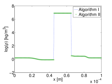
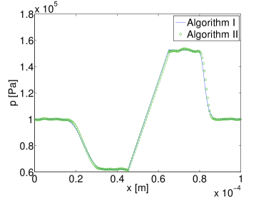
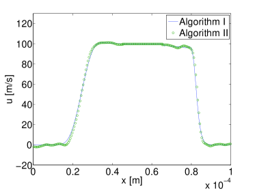
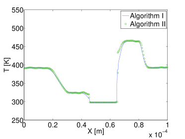
Figure 1: Test1: Logarithm of density(top left), pressure(top right), velocity(bottom left) and temperature(bottom right) for a Knudsen number of 0.0045. The solid lines are results from Algorithm I, the circles are from Algorithm II.

The initial number of gas molecules is $5000$ per cell of size $\Delta x$ for the simulation of the Boltzmann equation. We observe in figure 1 that the solutions obtained from the coupling of the Boltzmann and the incompressible Navier-Stokes equations (Algorithm II) match with the solutions obtained from the coupling of the compressible and incompressible Navier-Stokes equations (Algorithm I).

As in [CFA00] we notice that the liquid droplet moves to the right causing a compression wave in the gas ahead of it and an expansion wave behind it. Moreover, the gas is heated ahead of droplet and cooled behind it. To a very good approximation, the pressure profile inside the droplet is linear. This is expected and can be explained by the following argument. The liquid is decelerated by compressing the gas volume at its right. By the equivalence principle of general relativity, an acceleration (or deceleration) is equivalent to the action of a gravitational field. Therefore a linear hydrostatic pressure profile as in a quiescent liquid in a gravitational field is found.

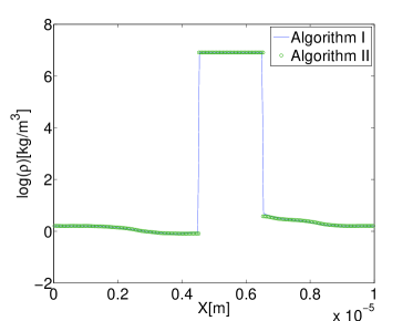
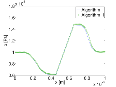
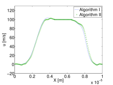
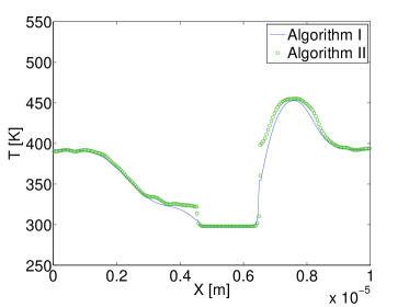
Figure 2: Test1: Logarithm of density(top left), pressure(top right), velocity(bottom left) and temperature(bottom right) for a Knudsen number of 0.045. The solid lines are results from Algorithm I, the circles are from Algorithm II.

Next, we consider a $10$ times smaller domain $\Omega=[0,1\times 10^{-5}~{}m]$ and the same initial values as above. Initially a liquid droplet occupies the domain $\Omega_{l}=[4\times 10^{-6}~{}m,6\times 10^{-6}~{}m]$, while the gas occupies the rest of the domain. The characteristic length is taken as the size of the droplet, which is equal to $2\times 10^{-6}$, giving a Knudsen number $\epsilon=0.045$. The simulation is stopped after a time $t=5.2\times 10^{-9}~{}s$. The results are plotted in figure 2 and show similar trends as the curves in figure 1. However, at such values of the Knudsen number first deviations from the results of continuum theory become visible.

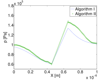
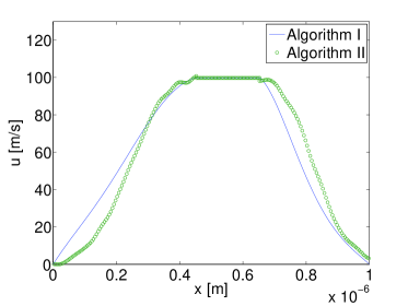
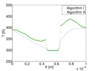
Figure 3: Test1: Logarithm of density(top left), pressure(top right), velocity(bottom left) and temperature(bottom right) for a Knudsen number of 0.45. The solid lines are results from Algorithm I, the circles are from Algorithm II.

We have further increased the Knudsen number by decreasing the computational domain and characteristic length by a factor of 10. In this case we have $\epsilon=0.45$, and simulation was stopped after $t=5.2\times 10^{-10}~{}s$. We have plotted the results in figure 3. For this Knudsen number we see that the solutions from the coupling algorithm I significantly deviate from the ones obtained from coupling algorithm II. This is, as expected, due to the failure of the compressible Navier-Stokes equations for larger Knudsen numbers. A constant velocity and a linear pressure profile are obtained inside the liquid. It also becomes apparent that the solution of the Boltzmann equation yields much more pronounced jumps in the temperature fields than that of the Navier-Stokes equations, similar as in the case of Sod’s 1D shock tube problem [TKH09].

5.2 Test 2

The second test case is also taken from paper of Caiden et al [CFA00], where the authors have considered only the Euler equations without the energy equation. We again consider the computational domain $\Omega=[0~{}m,1\times 10^{-4}~{}m]$. The liquid initially occupies the domain $\Omega_{l}=[4\times 10^{-5}~{}m,6\times 10^{-5}~{}m]$, and the rest of the domain is filled with gas. A shock wave is initially located at $x=1\times 10^{-5}~{}m$, with a post shock state $p_{g}(0,x)=148407.3~{}Pa,u_{g}(0,x)=89.981~{}m/s$ and $\rho_{g}(0,x)=2.214~{}kg/m^{3}$. On the right of $x=1\times 10^{-5}~{}m$ the initial state is given as $p_{g}(0,x)=98066.5~{}Pa,u_{g}(0,x)=0~{}m/s$ and $\rho_{g}(0,x)=1.58317~{}kg/m^{3}$. The initial temperature of the gas is again computed from the equation of state. The characteristic length is equal to $2\times 10^{-5}~{}m$. The pre- and post-shock Knudsen numbers are $0.00259$ and $0.00696$, respectively. The initial conditions for the liquid are $p_{l}=98066.5~{}Pa,u_{l}=0~{}m/s,T_{l}=298~{}K$. At first, we first consider a liquid density of $\rho_{l}=1000~{}kg/m^{3}$.

The boundary conditions for the compressible Navier-Stokes equations are $u_{g}(t,a)=89.981~{}m/s,T_{g}(t,a)=T(0,a)$, $T_{g}(t,b)=T_{g}(0,b)$, and we assume a vanishing velocity gradient at $x=b$.

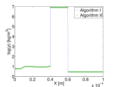
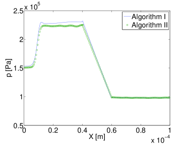
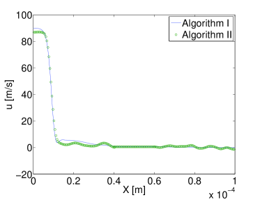
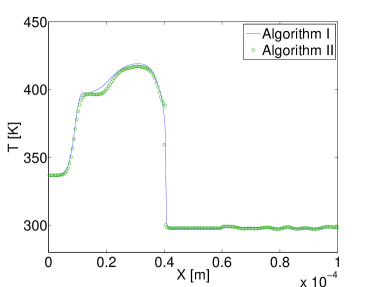
Figure 4: Test 2: Logarithm of density(top left), pressure(top right), velocity(bottom left) and temperature(bottom right) for a liquid density $\rho_{l}=1000~{}kg/m^{3}$ at time $t=1.75\times 10^{-7}~{}s$. The solid lines are results from Algorithm I, the circles are from Algorithm II.

For the Boltzmann equation we generate gas molecules in two ghost cells at the left boundary $x=a=0$ according to a Maxwellian with the initial parameters $\rho_{l}(0,a),{\bf u}_{g}(0,a)=(89.981,0,0)~{}m/s$ and $T_{g}(0,a)$. Similarly, we generate gas molecules in two cells at the right boundary $x=b$ according to a Maxwellian distribution with the parameters $\rho_{g}(0,b),T_{g}(0,b)$. The mean velocity ${\bf u}_{g}(t,b)$ is extrapolated from the neighboring cells at the left. After the free flow step, if gas molecules leave the boundaries at $a$ and $b$ we delete them. We note that we stopped the simulation before the wave reached the right boundary so that the mean velocity is still zero at this time. We have plotted the results at time $t=1.75\times 10^{-7}~{}s$ in figure 4. One can observe that the shock wave travels to the right hitting the droplet, causing reflected as well as transmitted waves. The reflected wave is clearly visible in the pressure and the temperature plots of figure 4, while both of the waves can be seen in figure 5. Again, the pressure profile is linear inside the droplet, however, with a reversed slope compared to the first test case. This originates from the fact that due to the interaction with the shock wave the accelaration of the droplet is now positive. The solutions obtained from both algorithms are very close to each other.

In figure 5 we have plotted the results from the same simulations with an liquid density $\rho_{l}=10~{}kg/m^{3}$ at the same time $t=1.75\times 10^{-7}~{}s$. It becomes apparent that for this lower liquid density the droplet has a lower inertia and is more easily displaced to the right. Compared to the initial state, the physical fields of the fluids have now been altered in almost the entire domain. Again, we see a good agreement of the solutions obtained from the coupling algorithms I and II.

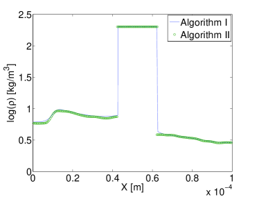
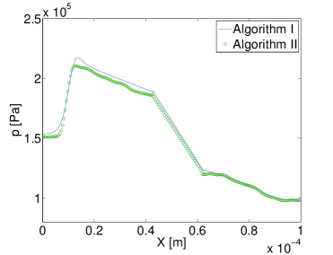
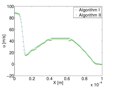
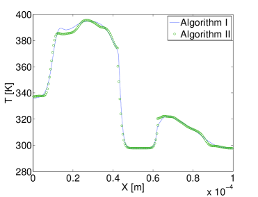
Figure 5: Test 2: Logarithm of density(top left), pressure(top right), velocity(bottom left) and temperature(bottom right) for a liquid density $\rho_{l}=10~{}kg/m^{3}$ at time $t=1.75\times 10^{-7}~{}s$. The solid lines are results from Algorithm I, the circles are from Algorithm II.

The above results are for the continuum gas regime. As expected, for the rarefied regime we see a discrepancy of the solutions obtained from algorithms I and II as in Test 1 for the largest Knudsen number. We do not explicitly present the corresponding results in this article.

5.3 Test 3

In the final test case we again consider the same computational domain as in Test 2. The liquid droplet is initially at rest, occupying the domain $\Omega_{l}=[2\times 10^{-5}~{}m,3\times 10^{-5}~{}m]$, while the rest of the domain is filled with gas. A similar test case has been studied in [FMO98] for a unit interval. Initially, the gas is in thermal equilibrium with the initial state ${\bf u}_{g}(0,x)=(0,0,0)~{}m/s,~{}T_{g}(0,x)=298~{}K$, and a spatially varying density $\rho_{g}(0,x)$. We assume $\rho_{g}(0,x)=1~{}kg/m^{3}$ at the left of the droplet and a four times smaller value at the right of it. This means that the pressure at the left of the droplet is four times larger than at the right. The characteristic length is $1\times 10^{-5}~{}m$, and the Knudsen numbers at the left and right of the droplet are $0.011$ and $0.044$, respectively. The initial values for the liquid are $u_{l}(0,x)=0m/s,~{}T_{l}(0,x)=298~{}K$, and the pressure is equal to the initial value in the gas at the right side of the droplet. We set the liquid density $\rho_{l}=10~{}kg/m^{3}$. The boundary conditions are the same as in Test 1.

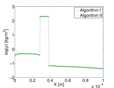
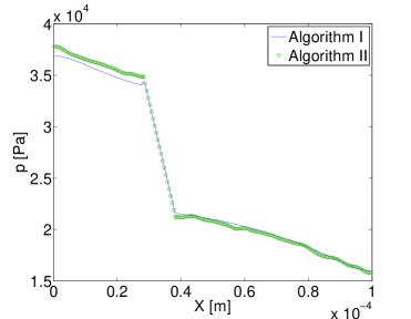
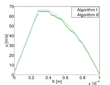
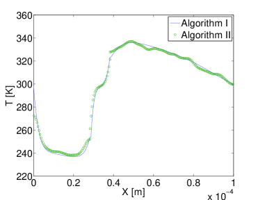
Figure 6: Test 3: Logarithm of density(top left), pressure(top right), velocity(bottom left) and temperature(bottom right) for a liquid density $\rho_{l}=10~{}kg/m^{3}$ at time $t=2.218\times 10^{-7}~{}s$. The solid lines are results from Algorithm I, the circles are from Algorithm II.

In figure 6 we have plotted the density, pressure, velocity and temperature after a short time $t=2.218\times 10^{-7}~{}s$. We see that the droplet has been slightly pushed to the right. The pressure on the left is higher. The gas has started to cool down on the left, and on the right it is getting compressed, resulting in a temperature increase.

At a later time $t=5.678\times 10^{-7}~{}s$ (figure 7) we observe that the compression on the right has further increased and the gas has been further heated. Now the pressure on the right is higher causing a slowing down of the droplet. Going along with the transition from droplet accelaration to deceleration is a reversal of the slope of the pressure profile inside the droplet. Later it will bounce back to the left. We observe that at both time levels the solutions obtained with both algorithms are in good agreement.

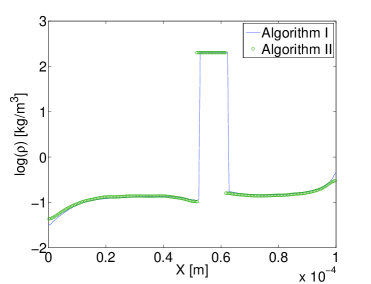
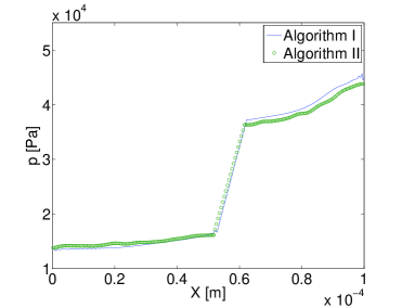
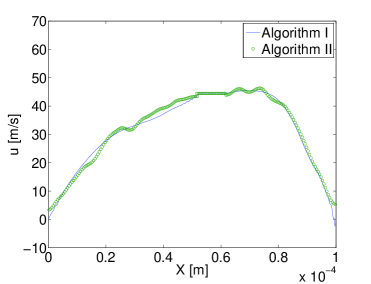
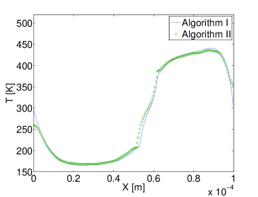
Figure 7: Test 3: Logarithm of density(top left), pressure(top right), velocity(bottom left) and temperature(bottom right) for a liquid density $\rho_{l}=10~{}kg/m^{3}$ at time $t=5.678\times 10^{-7}~{}s$. The solid lines are results from Algorithm I, the circles are from Algorithm II.

At a still later time ($t=9.938\times 10^{-7}~{}s$) we see that the droplet is already pushed to the left, as displayed in figure 8. At this time we see some discrepancy between algorithms I and II. This may be due to statistical fluctuation in the Boltzmann domain. However, the solutions are still comparable. If we compute further, the droplet will bounce back at the right boundary, and this oscillatory process will continue.

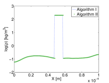
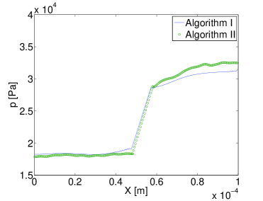
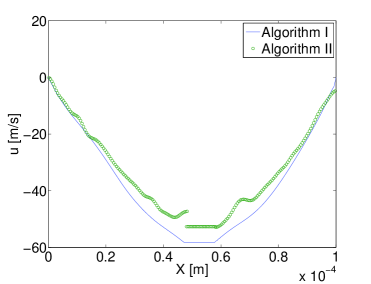
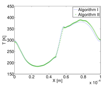
Figure 8: Test 3: Logarithm of density(top left), pressure(top right), velocity(bottom left) and temperature(bottom right) for a liquid density $\rho_{l}=10~{}kg/m^{3}$ at time $t=9.938\times 10^{-7}~{}s$. The solid lines are results from Algorithm I, the circles are from Algorithm II.

Similarly, for the rarefied gas regime, the solutions from Algorithms I and II do not match due to the breakdown of the continuum hypothesis inside the gas domain. As in Test 2 we do not present the results for larger Knudsen numbers.

6 Conclusion and Outlook

We have presented a coupling algorithm for a moving liquid phase inside a rarefied gas. The liquid phase is modeled by the incompressible Navier-Stokes equations, while the rarefied gas phase is modeled by the Boltzmann equation. The transport equations in the liquid are solved by a meshfree Lagrangian particle method, the Boltzmann equation by a DSMC type of particle method. Liquid particles overlap with the Boltzmann cells and the gas-liquid interface is determined from the particles at the boundary of the liquid domain. Interface boundary conditions are derived and a coupling algorithm for solving the Boltzmann equation in combination with the incompressible Navier-Stokes equations is presented. To validate the coupling between the rarefied gas and the liquid we have modeled the gas by the compressible Navier-Stokes equations. Both the compressible and incompressible Navier-Stokes equations are solved by a meshfree Lagrangian particle method, called the Finite Pointset Method (FPM), where the gas and liquid particles are distinguished by assigning different flags. We have also derived and implemented the interface boundary conditions for the compressible and incompressible Navier-Stokes equations which are well understood and widely used. In the continuum regime we have shown that the coupled solutions of the compressible and incompressible Navier-Stokes equations match well with the coupled solutions of the Boltzmann and the incompressible Navier-Stokes equations.

Future work will concentrate on the extension of the code to higher-dimensional problems, especially to the simulation of nano bubbles surrounded by an aqueos phase. Moreover, the method will be extended to simulate two-phase flows with evaporation and condensation [BS04, HW08].