A model for shock wave chaos

Abstract

We propose the following model equation:

$$u_{t}+\frac{1}{2}\left(u^{2}-uu_{s}\right)_{x}=f\left(x,u_{s}\right),$$

that predicts chaotic shock waves. It is given on the half-line $x<0$ and the shock is located at $x=0$ for any $t\geq 0$. Here $u_{s}\left(t\right)$ is the shock state and the source term $f$ is assumed to satisfy certain integrability constraints as explained in the main text. We demonstrate that this simple equation reproduces many of the properties of detonations in gaseous mixtures, which one finds by solving the reactive Euler equations: existence of steady traveling-wave solutions and their instability, a cascade of period-doubling bifurcations, onset of chaos, and shock formation in the reaction zone.

Shock waves arise in a wide range of physical phenomena: gas dynamics, shallow-water flows, supernovae, stellar winds, traffic flows, quantum fluids, and many others. The dynamics of shock waves can be quite intricate and difficult to analyze due to the difficult nature of the hyperbolic conservation laws that govern their evolution. The theory of shock waves has a rich history beginning with the fundamental contributions by Riemann in the middle of the 19th century. Nevertheless, numerous open questions remain regarding the shock dynamics, especially when classical gas-dynamical shock waves interact with additional physical or chemical phenomena, such as magnetic and gravitational fields, chemical reactions, radiation, and others.

Our focus in this Letter is on one fascinating feature of a shock wave propagating in a chemically active medium, namely shock-wave chaos. This is a phenomenon wherein the shock propagates with its speed oscillating chaotically about a certain average. It has previously been demonstrated to occur in gaseous detonations, by solving the reactive Euler equations Ng2005 ; HenrickAslamPowers2006 . Detonations are shock waves in reactive mixtures that are sustained by the chemical energy release in the mixture; the reactions, in turn, are triggered and sustained by the heating provided by the shock compression.

Analytical and numerical difficulties associated with solving the reactive Euler equations motivated the introduction of simple analog models, with the aim of capturing the essential nature of observed detonation shocks. As it is well-known, Burgers burgers1948mathematical introduced his equation, $u_{t}+uu_{x}=u_{xx}$ (where the subscripts $t$ and $x$ indicate partial derivatives), now a hallmark of hyperbolic differential equations and shock wave theory, in the hope of capturing the essential nature of turbulence with a simple and tractable model. Following a similar idea, Fickett Fickett:1979ys ; Fickett1985 and shortly after him Majda Majda:1980zr , introduced simple analog models for detonations in the hope of gaining some insight into the complicated behavior of detonation waves, as observed in experiment and numerical simulations. Fickett’s model is a modification of the Burgers’ equation, which introduces the effects of chemical energy release. It takes the form:

$$u_{t}+\frac{1}{2}(u^{2}+q\lambda)_{x}=0,\quad\lambda_{t}=\omega(\lambda,u),$$ (1)

where $u$ is the primary unknown mimicking density, temperature, or pressure, $\omega$ is a rate function, and $q$ is a constant playing the role of a chemical energy release. The chemistry here is represented by an irreversible reaction $reactants\rightarrow products$, with $\lambda$ being a normalized concentration of reaction products. At the shock, $\lambda=0$ and $\lambda$ increases through the reaction zone to reach $\lambda=1$ in the products.

Fickett’s model has been shown to reproduce some of the features of detonations Fickett:1979ys ; fickett1985stability ; Fickett1985 , most notably the steady-state structures. Still, the key unstable character of detonations had not been reproduced within this model until Radulescu and Tang Radulescu:2011fk extended it to a two-step chemistry with an inert induction zone followed by an energy-releasing reaction zone. In Radulescu:2011fk , the authors were able to reproduce, with their analog model, the complexity of chaotic detonations in the Euler equations.

In this Letter, we propose a model consisting of a single equation that predicts steady traveling wave solutions, instability through a Hopf bifurcation, and a sequence of period-doubling bifurcations with subsequent chaotic dynamics. The onset of chaos in our equation appears to follow the same scenario as in the logistic map may1976simple . For the reactive Euler equations and the Fickett’s analog model, the same scenario has been found HenrickAslamPowers2006 ; Radulescu:2011fk . We note that even though our model is still an analog, it is close to the weakly nonlinear model of Rosales and Majda RosalesMajda:1983ly , which is rationally derived from the Euler equations rather than postulated as the Fickett’s (or Majda’s) models. However, our emphasis here is not on the precise relationship of our model to the Euler equations, but rather on presenting what we believe is the simplest partial differential equation that is capable of capturing much of the richness of detonations in the reactive Euler equations.

Our model is the following partial differential equation:

$$u_{t}+\frac{1}{2}\left(u^{2}-uu_{s}\right)_{x}=f\left(x,u_{s}\right),$$ (2)

for $x<0$ and $t\geq 0$, with an appropriate initial condition, $u\left(x,0\right)$. Here $u_{s}\left(t\right)=u\left(0,t\right)$ is the boundary value of the solution, which is not prescribed but follows by solving (2), as explained below. The source term $f$ needs to satisfy certain integrability conditions, as also explained further below.

Equation (2) is a simple model for the reaction zone of a detonation moving into a uniform state, in coordinates attached to the leading shock. This can be seen by application of the Rankine-Hugoniot shock conditions (see, e.g. CourantFriedrichs ) at $x=0$, for (2) extended by taking $f=0$ and $u=0$ for $x>0$. Indeed, the shock condition

$$-V\left[u\right]+\frac{1}{2}\left[u^{2}\right]-\frac{1}{2}u_{s}\left[u\right]=0,$$ (3)

where $V$ is the shock speed and $[z]=z^{+}-z^{-}$ is the jump of $z$ across the shock (so that $\left[u\right]=-u_{s}$ and $\left[u^{2}\right]=-u_{s}^{2}$), yields $V=0$. We assume that the shock satisfies the usual Lax entropy conditions leveque1994numerical , so that the characteristics from both sides of the shock converge on the shock. That is,

$$\frac{dx}{dt}|_{0-}=\left(u-\frac{u_{s}}{2}\right)_{x=0-}=\frac{u_{s}}{2}>0\quad\mbox{and }$$ (4)

$$\frac{dx}{dt}|_{0+}=\left(u-\frac{u_{s}}{2}\right)_{x=0+}=-\frac{u_{s}}{2}<0,$$ (5)

which require that $u_{s}>0$. Therefore, no boundary condition at $x=0$ is necessary. Finally, we remark that $u_{s}$ is a measure of the shock strength, since $\left[u\right]=-u_{s}$, and for that reason we will analyze $u_{s}\left(t\right)$ in what follows when describing the shock dynamics.

The most unusual feature of (2) is that the equation contains in it the boundary value of the unknown, $u_{s}\left(t\right)$. This is in fact the key reason for the observed complexity of the solutions and has a simple physical interpretation: the boundary information from $x=0$ is propagated instantaneously throughout the solution domain, $x<0$, while there is a finite-speed influence propagating from the reaction zone back toward the shock along the characteristics of (2). Importantly, in the Euler equations, this situation occurs in a weakly nonlinear reactive shock wave where the flow behind the shock is nearly sonic relative to the shock RosalesMajda:1983ly . One family of acoustic characteristics is then nearly parallel to the shock, representing the slow part of the wave moving toward the shock. The second family moves away from the shock and represents the influence of the shock on the whole post-shock flow. This occurs on a much faster time scale than the information flow toward the shock. Our model makes this fast influence instantaneous.

One can easily obtain the steady-state solution $u_{0}\left(x\right)$ of (2) by solving

$$\frac{1}{2}\left(u_{0}^{2}-u_{0}u_{0s}\right)^{\prime}=f\left(x,u_{0s}\right),$$ (6)

where the prime denotes the derivative with respect to $x$ and the subscript $s$ denotes the shock state. The solution is

$$u_{0}\left(x\right)=\frac{u_{0s}}{2}+\sqrt{\frac{u_{0s}^{2}}{4}+2\int_{0}^{x}f\left(y,u_{0s}\right)dy}.$$ (7)

The choice of the steady-state shock strength

$$u_{0s}=2\sqrt{2\int_{-\infty}^{0}f\left(y,u_{0s}\right)dy}$$ (8)

corresponds to the Chapman-Jouguet speed in detonation theory FickettDavis79 , since then the characteristic speed at $x=-\infty$ is $u_{0}\left(-\infty\right)-u_{0s}/2=0$ indicating that the sonic point is reached only at an infinite distance from the shock. This situation is analogous to the commonly used simple-depletion kinetics in gaseous detonations FickettDavis79 .

If one substitutes (8) into (7), the result is

$$u_{0}\left(x\right)=\frac{u_{0s}}{2}+\sqrt{2\int_{-\infty}^{x}f\left(y,u_{0s}\right)dy}.$$ (9)

Clearly, for the solution $u_{0}\left(x\right)$ to be real and bounded, one must require that

$$0\leq\int_{-\infty}^{x}f\left(y,u_{0s}\right)dy<\infty$$ (10)

for any $-\infty<x\leq 0$. This is the constraint on $f$ that we mentioned earlier in the Letter. There may be other or additional, more stringent conditions on $f$ in other circumstances, but their discussion is outside the scope of this Letter.

Now we explore the fully nonlinear and unsteady solutions of (2), for the particular case

$$f=\frac{q}{2}\frac{1}{\sqrt{4\pi\beta}}\exp\left[-\frac{\left(x-x_{f}\left(u_{s}\right)\right)^{2}}{4\beta}\right].$$ (11)

The function $f$ peaks at $x_{f}$, chosen here as $x_{f}=-k\left(u_{0s}/u_{s}\right)^{\alpha},$ where $k>0$ and $\alpha\geq 0$ are parameters. We first rescale the variables as follows: $u$ by $u_{0s}$, so that the dimensionless steady-state shock strength is $1$, length by $l=k$, and time by $\tau=l/u_{0s}$. From (9), putting in all the dimensionless variables and rescaling $\beta$ by $l^{2}$, we obtain (keeping the same notation for the dimensionless variables and parameters)

$$u_{0}\left(x\right)=\frac{1}{2}\left[1+\sqrt{\frac{1+\mathrm{erf}\left(\left(x+1\right)/2\sqrt{\beta}\right)}{1+\mathrm{erf}\left(1/2\sqrt{\beta}\right)}}\right],$$ (12)

where $\mathrm{erf}\left(x\right)$ is the error function. The dimensionless form of (2) is

$$u_{t}+\frac{1}{2}\left(u^{2}-uu_{s}\right)_{x}=a\exp\left[-\frac{\left(x+u_{s}^{-\alpha}\right)^{2}}{4\beta}\right],$$ (13)

where $a=1/\left[4\sqrt{4\pi\beta}\left(1+\mathrm{erf}\left(1/2\sqrt{\beta}\right)\right)\right]$. Equation (13) contains only two parameters now, $\alpha$ reflecting the shock-state sensitivity of the source function $f$ (an analog of the activation energy in detonations) and $\beta$ reflecting the width of $f$ (an analog of the ratio between the reaction-zone length and the induction-zone length).

In the computations below, we use the shock-fitting algorithm of HenrickAslamPowers2006 on a domain of length $L=10$ with $N=3000$ uniformly spaced grid points. We fix $\beta=0.1$ in all calculations and vary $\alpha$ to capture instability and bifurcations. When long-time data, such as the local maxima of $u_{s}\left(t\right)$ are needed, we compute until $t=6000$. Simulations start with the steady-state solution perturbed by numerical noise. In Fig. 1 one can see that a period doubling occurs as $\alpha$ is increased from $\alpha_{1}=4.70$ to $\alpha=4.85$. Below the critical value $\alpha_{c}\approx 4.04$, the steady solution is found to be stable.

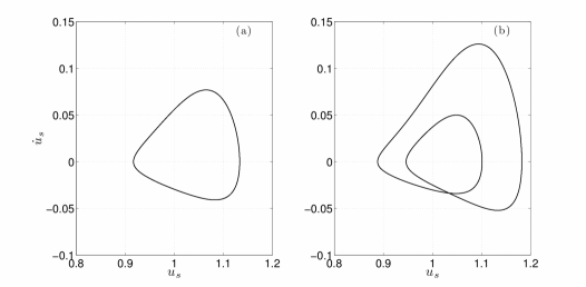
Figure 1: The limit cycles in the plane of the shock strength $u_{s}\left(t\right)$ vs $\dot{u}_{s}$ at $\alpha=4.70$ (a) and $\alpha=4.85$ (b).

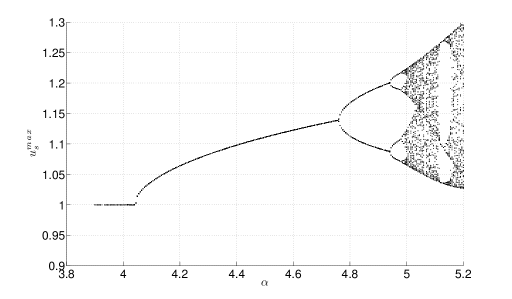
Figure 2: Values of the local maxima $u_{s}^{max}$ of the shock strength as a function of the parameter $\alpha$; $u_{s}^{max}$ are calculated at sufficiently large $t$ to make sure the solution has settled to its attractor.

If $\alpha$ is increased to large values, we observe that the reaction zone extends significantly initially, but subsequently shrinks. Importantly, as the reaction zone shrinks, another shock is formed within the reaction zone which then overtakes the lead shock at $x=0$, exactly analogous to what happens in the reactive Euler equations. Under these conditions, the dynamics is no longer smooth and must be analyzed differently. Therefore, we focus on moderately large $\alpha$, namely $\alpha<5.2$ for our particular choice of $\beta$, so that the dynamics is unstable, but no internal shock waves appear to form. Remarkably, as $\alpha$ is increased, we observe a sequence of period-doubling bifurcations that leads to chaotic solutions at $\alpha$ close to or slightly larger than $5$, as seen in Fig. 2. The onset of chaos apparently follows the same scenario as in the logistic map may1976simple ; strogatz1994nonlinear . The bifurcation diagram in Fig. 2 was computed by solving (13) until $t=6000$ for the range of $\alpha$ from $3.9$ to $5.2$, with an increment of $0.005$. For each $\alpha$, we find the maxima of $u_{s}\left(t\right)$ between $t=5000$ and $t=6000$ and plot them on the figure. Based on a sequence of three period doublings, we estimated the Feigenbaum constant $\delta$ feigenbaum1983universal to be about $4.5$. This is in rough agreement with the well-known value of $\delta=4.669...$ for the logistic map as well as that found for detonations strogatz1994nonlinear ; Ng2005 ; HenrickAslamPowers2006 ; Radulescu:2011fk .

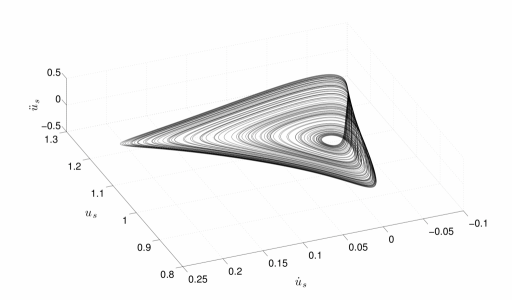
Figure 3: The chaotic attractor in the space of $u_{s}$, $\dot{u}_{s}$, and $\ddot{u}_{s}$ at $\alpha=5.1$.

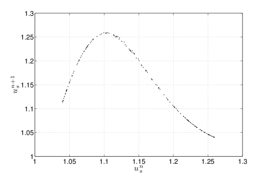
Figure 4: The Lorenz map showing consecutive local maxima ($u_{s}^{n},\,\,u_{s}^{n+1}$) of the shock strength $u_{s}\left(t\right)$ over large times (from $t=3000$ to $t=6000$) for the chaotic case at $\alpha=5.1$.

We plot the chaotic attractor at $\alpha=5.1$ in the space of $u_{s}$, $\dot{u}_{s}$, and $\ddot{u}_{s}$ as shown in Fig. 3. Its resemblance to the Rössler attractor Rossler1976 is evident. Interestingly, when we plot the local maxima of $u_{s}$ versus their prior values (i.e. the Lorenz map Lorenz1963 , see Fig. 4), the data fall almost on a curve. The curve also resembles the one for the Rössler attractor. These observations suggest that the shock-wave chaos arising from (2) is controlled by a low-dimensional process similar to that of a simple one-dimensional map$\--$just as it is the case with the Lorenz and Rössler attractors strogatz1994nonlinear .

- [1] J.M. Burgers. A mathematical model illustrating the theory of turbulence. Adv. Appl. Mech, 1(171-199):677, 1948.
- [2] R. Courant and K. Friedrichs. Supersonic Flow and Shock Waves. Springer-Verlag, New York, NY., 1976.
- [3] M.J. Feigenbaum. Universal behavior in nonlinear systems. Physica D: Nonlinear Phenomena, 7(1-3):16–39, 1983.
- [4] W. Fickett. Detonation in miniature. American Journal of Physics, 47(12):1050–1059, 12 1979.
- [5] W. Fickett. Introduction to Detonation Theory. University of California Press, Berkeley, CA, 1985.
- [6] W. Fickett. Stability of the square-wave detonation in a model system. Physica D: Nonlinear Phenomena, 16(3):358–370, 1985.
- [7] W. Fickett and W. C. Davis. Detonation. University of California Press, Berkeley, CA, 1979.
- [8] A. K. Henrick, T. D. Aslam, and J. M. Powers. Simulations of pulsating one-dimensional detonations with true fifth order accuracy. J. Comput. Phys., 213(1):311–329, 2006.
- [9] R.J. LeVeque. Numerical Methods for Conservation Laws. Birkhäuser Verlag AG, 1994.
- [10] E.N. Lorenz. Deterministic nonperiodic flow. J. Atmos. Sci, 20(130):130, 1963.
- [11] A. Majda. A qualitative model for dynamic combustion. SIAM Journal on Applied Mathematics, 41(1):70–93, 08 1980.
- [12] R.M. May. Simple mathematical models with very complicated dynamics. Nature, 261(5560):459–467, 1976.
- [13] H. Ng, A. Higgins, C. Kiyanda, M. Radulescu, J. Lee, K. Bates, and N. Nikiforakis. Nonlinear dynamics and chaos analysis of one-dimensional pulsating detonations. Combust. Theory Model, 9(1):159–170, 2005.
- [14] M.I. Radulescu and J. Tang. Nonlinear dynamics of self-sustained supersonic reaction waves: Fickett’s detonation analogue. Phys. Rev. Lett., 107(16), 2011.
- [15] R.R. Rosales and A. J. Majda. Weakly nonlinear detonation waves. SIAM Journal on Applied Mathematics, 43(5):1086–1118, 1983.
- [16] O.E. Rössler. An equation for continuous chaos. Physics Letters A, 57(5):397–398, 1976.
- [17] S.H. Strogatz. Nonlinear dynamics and chaos: With applications to physics, biology, chemistry, and engineering. Westview Pr, 1994.