The vertical motions of mono-abundance sub-populations in the Milky Way disk

Abstract

We present the vertical kinematics of stars in the Milky Way’s stellar disk inferred from SDSS/SEGUE G-dwarf data, deriving the vertical velocity dispersion, $\sigma_{z}$, as a function of vertical height $|z|$ and Galactocentric radius $R$ for a set of ‘mono-abundance’ sub-populations of stars with very similar elemental abundances $[\alpha\mathrm{/Fe}]$ and $[\mathrm{Fe/H}]$. We find that all mono-abundance components exhibit nearly isothermal kinematics in $|z|$, and a slow outward decrease of the vertical velocity dispersion: $\sigma_{z}\bigl{(}z,R\,|\,[\alpha\mathrm{/Fe}],[\mathrm{Fe/H}]\bigr{)}\approx\sigma_{z}\bigl{(}[\alpha\mathrm{/Fe}],[\mathrm{Fe/H}]\bigr{)}\times\exp\bigl{(}-(R-R_{0})/7\,\mathrm{kpc}\bigr{)}$. The characteristic velocity dispersions of these components vary from $\sim$ 15 km s^-1 for chemically young, metal-rich stars with solar $[\alpha\mathrm{/Fe}]$, to $\gtrsim 50$ km s^-1 for metal-poor stars that are strongly $[\alpha\mathrm{/Fe}]$-enhanced, and hence presumably very old. The mean $\sigma_{z}$ gradient $(\mathrm{d}\sigma_{z}/\mathrm{d}z)$ away from the mid-plane is only $0.3\pm 0.2$ km s^-1 kpc^-1. This kinematic simplicity of the mono-abundance components mirrors their geometric simplicity; we have recently found their density distribution to be simple exponentials in both the $z$ and $R$ directions. We find a continuum of vertical kinetic temperatures ($\propto\sigma^{2}_{z}$) as a function of $\bigl{(}[\alpha\mathrm{/Fe}],[\mathrm{Fe/H}]\bigr{)}$, which contribute to the total stellar surface-mass density approximately as $\Sigma_{R_{0}}(\sigma^{2}_{z})\propto\exp(-\sigma^{2}_{z})$. This and the existence of isothermal mono-abundance populations with intermediate dispersions (30 to 40 km s^-1) reject the notion of a thin–thick disk dichotomy. This continuum of disk components, ranging from old, ‘hot’, and centrally concentrated ones to younger, cooler, and radially extended ones, argues against models where the thicker disk portions arise from massive satellite infall or heating; scenarios where either the oldest disk portion was born hot, or where internal evolution plays a major role, seem the most viable. In addition, the wide range of $\sigma_{z}\bigl{(}[\alpha\mathrm{/Fe}],[\mathrm{Fe/H}]\bigr{)}$ combined with a constant $\sigma_{z}(z)$ for each abundance bin provides an independent check on the precision of the SEGUE-derived abundances: $\delta_{[\alpha\mathrm{/Fe}]}\approx 0.07$ dex and $\delta_{[\mathrm{Fe/H}]}\approx 0.15$ dex. The slow radial decline of the vertical dispersion presumably reflects the decrease in disk surface-mass density. This measurement constitutes a first step toward a purely dynamical estimate of the mass profile of the stellar and gaseous disk in our Galaxy.

1. Introduction

The spatial structure and kinematics of stars in the Milky Way’s disk appear to be complex, varying distinctly with the elemental abundances of different sub-populations: more metal-rich populations form thinner, kinematically cooler sub-components, while metal-poor and $[\alpha\mathrm{/Fe}]$-enhanced populations form thicker, kinematically hotter disk components (e.g., Fuhrmann, 1998; Chiba & Beers, 2000; Feltzing et al., 2003; Lee et al., 2011b; Bovy et al., 2012a). The elemental abundances of stars, in particular $[\mathrm{Fe/H}]$ and $[\alpha\mathrm{/Fe}]$, encode—albeit in complex ways—information about their age and birth location within the Galaxy (e.g., Schönrich & Binney, 2009). The present chemo-dynamical structure of the Milky Way’s stellar disk must reflect the combination of the orbits on which stars were formed, and the evolutionary changes that they underwent since, with the abundances being the best practical sub-population ‘tag’ that is preserved throughout the lifetime of a star. As such, the chemo-dynamical structure of our Galaxy’s disk holds unique clues toward understanding its formation and evolution. Because a good portion of stars in the present-day universe live in galaxies comparable to the Milky Way, and because the large majority of Milky Way stars live in the disk, dissecting and understanding our Galactic disk has broad implications for our understanding of galaxy formation.

In a recent paper, we have expanded on earlier work studying the Galactic disk as a function of elemental abundances, by showing that the geometric structure of the disk is relatively simple when viewed as a superposition of ‘mono-abundance’ sub-populations (Bovy et al., 2012a, B12a hereafter) drawn from SDSS/SEGUE (Abazajian et al., 2009; Yanny et al., 2009): the density of any set of stars chosen to have a narrow range in $[\alpha\mathrm{/Fe}]$ and $[\mathrm{Fe/H}]$ appears to be well-described by a single exponential in both the radial and vertical directions. In particular, B12a found that the (single) vertical scale height, $h_{z}$ at a given $\bigl{(}[\alpha\mathrm{/Fe}],[\mathrm{Fe/H}]\bigr{)}$ varies systematically with these two abundance parameters, in the sense that populations that are metal poor and $\alpha$-enhanced, or $\alpha$-old, are vertically thicker. It had been established that the thicker disk components are $\alpha$-old (Fuhrmann, 1998; Prochaska et al., 2000; Bensby et al., 2003), but our recent work shows that the reverse also holds: $\alpha$-old sub-populations form thicker disk components than $\alpha$-young sub-populations. Furthermore, an analysis of the total amount of stellar mass in disk components of different thicknesses exhibits a continuous and monotonic distribution of disk thicknesses, rather than a simple thin–thick dichotomy (Bovy et al., 2012b).

In this present paper, we follow up on B12a by exploring the vertical kinematics, $p(v_{z}|z,R)$ or $\sigma_{z}(z,R)$, for mono-abundance sub-populations, in practice for subsets of G-type dwarfs from SDSS/SEGUE in a small range of $\bigl{(}[\alpha\mathrm{/Fe}],[\mathrm{Fe/H}]\bigr{)}$. The goals of this analysis are two-fold: first, to see how the distinct and simple spatial structure of mono-abundance sub-populations is reflected in the vertical motions of these sub-components; second, to lay the ground work for a dynamical analysis to determine the gravitational potential near the disk plane.

Beyond the immediate solar neighborhood ($\sim\,100-200$ pc, e.g., Flynn & Fuchs 1994, Nordström et al. 2004), the first determination of the vertical velocity dispersion profile was carried out by Kuijken & Gilmore (1989), who obtained nearly complete line-of-sight velocities for a sample of about 500 K-type dwarfs near the south Galactic pole. For this sample, with a fairly broad metallicity selection function, they found that the velocity dispersion profile, $\sigma_{z}(z)$, rose from $\sim 18$ km s^-1 near the mid-plane to $\sim 40$ km s^-1 at $\sim 1.3$ kpc above the plane. Fuchs et al. (2009) used proper motions of M-type stars from SDSS to confirm that the velocity dispersion exhibits a quite strong linear increase away from the disk mid-plane, finding an even stronger gradient. Bond et al. (2010) used photometric metallicity estimates to isolate a low-metallicity sample, which showed a considerably slower rise of $\sigma_{z}(z)$ away from the plane.

Much of the rise in $\sigma_{z}(z)$ found in these analyses is presumably attributable to a much higher fraction of low-metallicity stars well above the mid-plane, stars that form a kinematically hotter sub-component. This would also explain why the sample with a more restricted metallicity range (Bond et al., 2010) shows a shallower rise toward large $|z|$. Just recently, Liu & van de Ven (2012) confirmed this interpretation, using preliminary $[\alpha\mathrm{/Fe}]$ values for SDSS/SEGUE G-dwarf spectra. They show that the vertical dispersion profile becomes approximately isothermal, when splitting the sample in a number of $[\alpha\mathrm{/Fe}]$ bins. In this paper, we expand on these studies, by determining $\sigma_{z}(z)$ for sub-populations in a narrow range in $\bigl{(}[\alpha\mathrm{/Fe}],[\mathrm{Fe/H}]\bigr{)}$, which turn out to be exquisitely close to isothermal, i.e., $\sigma_{z}\bigl{(}z|R,[\alpha\mathrm{/Fe}],[\mathrm{Fe/H}]\bigr{)}\approx$ constant.

When combined with the spatial structure in the radial and vertical direction, the kinematics of these mono-abundance populations form the basis for exploring the viability of various internal or external disk evolution and disk heating mechanisms. The vertical density distribution and kinematics of these mono-abundance populations can also provide powerful constraints on the gravitational potential perpendicular to the plane, for two reasons. First, components with a simple spatial and kinematic distribution function are more easily modeled, and a density profile $\nu_{*}(z|[\alpha\mathrm{/Fe}],[\mathrm{Fe/H}])\propto\exp{\bigr{(}-z/h_{z}([\alpha\mathrm{/Fe}],[\mathrm{Fe/H}])\bigr{)}}$, $\sigma_{z}(z|[\alpha\mathrm{/Fe}],[\mathrm{Fe/H}])\approx$ constant is about as simple as it could get. Second, all mono-abundance sub-components feel the same gravitational potential, and hence provide extensive mutual checks on the dynamical inferences.

The outline of this paper is as follows. In $\mathsection$ 2 we briefly summarize the properties of the data set, and in $\mathsection$ 3 we describe the approach to estimating $\sigma_{z}(z|[\alpha\mathrm{/Fe}],[\mathrm{Fe/H}])$. We then present the results of this analysis in $\mathsection$ 4, not only $\sigma_{z}(z|R_{\odot},[\alpha\mathrm{/Fe}],[\mathrm{Fe/H}])$ but also its dependence on Galactocentric radius. We also describe how our observations that the mono-abundance components are so nearly isothermal in the vertical direction and have such a strong dependence of the dispersion on $\bigl{(}[\alpha\mathrm{/Fe}],[\mathrm{Fe/H}]\bigr{)}$ can be used to assess the abundance errors of the SEGUE data, independent of all other existing constraints. In $\mathsection$ 5 we put these results into context and discuss their implications. We summarize our findings in $\mathsection$ 6.

2. SDSS/SEGUE G-dwarf data

Figure 1.— Vertical velocities as a function of Galactocentric radius (top panels) and vertical height (bottom panels) for the $\alpha$-young sample (left panels; $-0.3<[\mathrm{Fe/H}]<0.25,0.00<[\alpha\mathrm{/Fe}]<0.25$ ) and for the $\alpha$-old (right panels; $-1.5<[\mathrm{Fe/H}]<-0.25,0.25<[\alpha\mathrm{/Fe}]<0.50$) sample. The median and 16/84 quantiles of the distribution in bins of width $\approx 0.4$ kpc (as a function of $R$) and $\approx 150$ pc (as a function of $z$) are indicated by the solid line and the shaded regions, respectively.

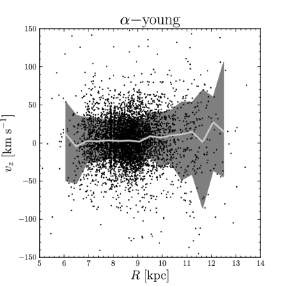
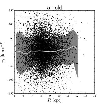
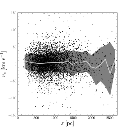
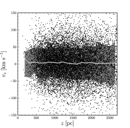
The sample on which we draw in this analysis is identical to the one used in B12a, but we now also use the stars’ line-of-sight velocities and proper motions explicitly. For an extensive description of the sample, we refer the reader to B12a, Yanny et al. (2009), and Lee et al. (2011b), and just summarize some salient points here: G-type dwarfs are the most extensive of the systematically targeted sub-samples in SEGUE to explore the Galactic disk; they are the most luminous tracers whose main-sequence lifetime is larger than the expected disk age at basically all metallicities. Their rich metal-line spectrum affords good velocity determinations ($\sim\!5$ to 10 km s^-1; Yanny et al. 2009), as well as good abundance ($[\alpha\mathrm{/Fe}],[\mathrm{Fe/H}]$) determinations ($\delta_{[\alpha\mathrm{/Fe}]}\sim 0.1$ dex, $\delta_{[\mathrm{Fe/H}]}\sim 0.2$ dex, Lee et al. 2008a, b; Allende Prieto et al. 2008; Schlesinger et al. 2010; Lee et al. 2011a; Smolinski et al. 2011, which we re-examine in this paper). Given the (metallicity-dependent) absolute magnitude of targeted G-type dwarfs with $0.48<(g-r)_{0}<0.55$, ranging from $4\lesssim M_{r}\lesssim 6$, the distances to the sample stars range from $0.6$ kpc to nearly 4 kpc. Stars somewhat closer to the disk plane are sampled by the lines of sight at lower Galactic latitudes, but the effective minimal distance limit of the stars (600 pc) implies that the vertical heights below one scale height ($|z|<h_{z}$) of the thinner disk components is not sampled by the data. As in B12a, we employ a signal-to-noise ratio cut of S/N $>15$, rather than the $S/N>20$ recommended by Lee et al. (2011a); we have explicitly checked that our results are the same when using S/N $>20$.

The specific analysis in this paper requires the height above the plane, the Galactocentric radius, and the vertical velocity and its error for each star. For a star at distance $d$ in the direction ($l,b$), i.e., with $\vec{d}=d\cdot(\cos l\cos b,\sin l\cos b,\sin b)$ in the Cartesian Galactic coordinate system, we have $|z|=|\vec{d}\cdot\vec{e_{z}}|$ and $R=|\vec{R_{0}}+\vec{d}-\vec{z}|$. We assume that the Sun’s displacement from the mid-plane is 25 pc toward the north Galactic pole (Chen et al., 2001; Jurić et al., 2008), and that the Sun is located at 8 kpc from the Galactic center (e.g., Bovy et al., 2009). We ignore distance uncertainties when using the spatial position of stars in the sample in the analysis below, as the distance uncertainties are much smaller than the spatial gradients in the quantities of interest. We do, however, propagate the distance uncertainties into the velocity uncertainties.

The motions in the $z$-direction are a combination of the line-of-sight velocities, $v_{\mathrm{los}}$, and the proper motions in the $b$-direction, $\mu_{b}$: $v_{z}(b,d,v_{\mathrm{los}})=v_{\mathrm{los}}\,\sin b+d\,\mu_{b}$; we assume that the Sun’s vertical motion is 7.25 km s^-1 (Schönrich et al., 2010). Given that we expect $\sigma_{z}\lesssim 20$ km s^-1 for the coldest disk components, the $v_{z}$ errors, $\delta_{v_{z}}$, matter greatly, both because for stars of lower signal-to-noise ratio $\delta_{v_{\mathrm{los}}}\approx 10$ km s^-1, and because with typical $\delta_{\mu_{b}}\sim 3.5$ mas yr^-1 (Munn et al., 2004) the error contribution from the proper motion $\delta_{v_{z}|\mu_{b}}=15\,\mathrm{km\ s}^{-1}\cdot[d/1\,\mathrm{kpc}]\cdot[\delta_{\mu_{b}}/(3.5\,\mathrm{mas\ yr}^{-1})]$ rises linearly with distance, becoming dominant beyond 1 kpc. The uncertainties in $v_{z}$ for each star are derived by marginalizing over the line-of-sight velocity, proper motion, and distance errors; the distance errors in turn are obtained by marginalizing over the color and apparent-magnitude errors that enter the photometric distance relation (Equation (A7) of Ivezić et al. 2008, see also B12a), which is assumed to have an intrinsic scatter of 0.1 mag in the distance modulus. It is important to note that for the present analysis, the detailed understanding of the sampling function that was painful and crucial for B12a and Bovy et al. (2012b) plays no role here, as long as one can assume that the vertical velocities of the targeted G-type dwarfs at a given $l,b,r,g-r,$ and $[\alpha\mathrm{/Fe}]$, $[\mathrm{Fe/H}]$ have kinematics identical to their untargeted kin with those same non-kinematic parameters.

As discussed in detail in Section 5.1 of B12a, the distances we use here could be systematically under- or over-estimated by up to 10 % due to the presence of unresolved multiple systems or the use of a different distance calibration, respectively. This systematic distance uncertainty can propagate into the vertical velocities for stars in our sample through the dependence on the distance of the velocity component that is tangential to the line of sight. In what follows we discuss the impact of this systematic distance error on our results, finding that it does not significantly impact any of our results.

We begin with a SEGUE G-dwarf sample that has about 28,000 stars with acceptably well-determined measurements, but here we only use those 23,767 stars that fall within well-populated ‘mono-abundance’ bins in the ($[\mathrm{Fe/H}]$,$[\alpha\mathrm{/Fe}]$) plane (B12a; a bin is well-populated when it contains more than 100 stars; the maximum number of stars in a bin is 789). Figure 1 provides a basic representation of the data used in the subsequent analysis: the top panels show $v_{z}$ vs. $R$ for a broadly selected $\alpha$-young (left; $-0.3<[\mathrm{Fe/H}]<0.25,0.00<[\alpha\mathrm{/Fe}]<0.25$) and $\alpha$-old (right; $-1.5<[\mathrm{Fe/H}]<-0.25,0.25<[\alpha\mathrm{/Fe}]<0.50$) sample, respectively. The bottom panels show $v_{z}$ vs. $z$. This figure immediately illustrates that, as expected, the vertical velocity dispersion of the $\alpha$-old sample is considerably higher than that of the $\alpha$-young sample, and that there are no strong changes of the velocity dispersion with either distance from the plane or Galactocentric radius. The spatial distribution of these two coarse-binned abundance-selected samples is shown in Figure 3 of B12a. That figure shows that the sample spans multiple kpc in $R$ for $\alpha$-young and $\alpha$-old subsamples and that all subsamples cover the $(R,z)$ plane fairly well. Thus, we can model the full $(R,z)$ dependence of $\sigma_{z}$ in each mono-abundance bin.

3. Mapping the vertical velocity dispersion of G-type dwarfs

We now describe how we estimate the vertical velocity distribution profile for each mono-abundance sub-population, characterized by $\sigma_{z}(z,R|[\alpha\mathrm{/Fe}],[\mathrm{Fe/H}])$, exploiting the discrete information we have: $\{v_{z,i},\delta_{v_{z,i}}|z_{i},R_{i}\},i=1,N_{j}$ for each abundance bin $([\mathrm{Fe/H}]_{j},[\alpha\mathrm{/Fe}]_{j})$. Note that we model the velocity distribution as Gaussians, rather than directly measuring it as the second moment of the observed vertical velocities $\sum_{i}{(v_{z,i}-\langle v_{z}\rangle)^{2}/N}$ in spatial bins. This allows us to take the individual observational uncertainties $\delta_{v_{z,i}}$ into account and to deal with outliers. As the SEGUE data selection is kinematically unbiased and we are only interested in the distribution of vertical velocities as a function of position, we do not have to correct for any selection effects.

We presume that the vertical velocity distribution $p(v_{z}|z,R,[\mathrm{Fe/H}]_{j},[\alpha\mathrm{/Fe}]_{j})$ can be described by

$$\begin{split}p(v_{z}|z,R,\vec{p}_{j},\delta_{v_{z,i}}\,)=&(1-\epsilon_{j})\cdot\frac{1}{\sqrt{2\pi}\sigma_{z}(z,R\,|\,\vec{p}_{j},\delta_{v_{z,i}})}\\ &\qquad\qquad\cdot\exp{\Bigl{(}\frac{-v^{2}_{z}}{2\sigma^{2}_{z}(z,R\,|\,\vec{p}_{j},\delta_{v_{z,i}})}}\Bigr{)}\ \\ &+\epsilon_{j}\cdot p_{\mathrm{backgr}}(z,R\,),\end{split}$$ (1)

where $\vec{p}_{j}$ is the vector of parameters to be fit in each abundance bin $j$ and $p_{\mathrm{backgr}}(z,R)$ is a simple normalized interloper model (reflecting data analysis outliers and halo contamination). Specifically, for $p_{\mathrm{backgr}}(z,R)$ we choose a normalized Gaussian with a dispersion of 100 km s^-1, convolved with the observational uncertainty $\delta_{v_{z,i}}$, and $\epsilon_{j}$ is a free parameter that is the fraction of stars deemed interlopers. In what follows we will fit $\vec{p}_{j}$ and $\epsilon_{j}$ for each abundance bin independently. To reduce notational clutter, we will mostly drop the ‘$j$’ index with the assumptions that the parameters $\vec{p}$ and $\epsilon$ are fitted in the discrete $([\mathrm{Fe/H}]_{j},[\alpha\mathrm{/Fe}]_{j})$ abundance bins.

Figure 2.— Best-fit vertical velocity dispersion profile, $\sigma_{z}(z)$, at $R_{0}$ and slope of the velocity dispersion as a function of $|z|$, evaluated at the median vertical height $z_{1/2}$ for each bin, as a function of $[\mathrm{Fe/H}]$ and $[\alpha\mathrm{/Fe}]$ (top panels) in bins of width 0.1 in $[\mathrm{Fe/H}]$ and 0.05 in $[\alpha\mathrm{/Fe}]$. The bottom panels show the best-fit velocity dispersion profile (modeled as a 2nd-order polynomial) as a function of height above the mid-plane for each bin in the top panels with a 20 % or better determination of $\sigma_{z}(z_{1/2})$, color-coded for each point in ($[\mathrm{Fe/H}]$,$[\alpha\mathrm{/Fe}]$), according to $[\alpha\mathrm{/Fe}]$ (left panel) and $[\mathrm{Fe/H}]$ (right panel). The velocity dispersion in the bottom panels is evaluated over the range in vertical height that contains 95 % of the data sample for each mono-abundance bin; the median height of the observed data is indicated by a dot in the bottom panels. Each ($[\mathrm{Fe/H}]$,$[\alpha\mathrm{/Fe}]$) bin contains at least 100 stars, and the width of each line in the bottom panels is proportional to the square root of the number of data points.

Figure 3.— Parameter uncertainties for the quadratic velocity dispersion profile fits for six representative mono-abundance bins: the peak and one-sigma uncertainty ellipses for each ($[\mathrm{Fe/H}]$,$[\alpha\mathrm{/Fe}]$) bin’s PDF for the parameters of the vertical velocity dispersion are shown for 2D projections of the 5D parameter space. Clockwise from the top, left panel these are: slope vs. velocity dispersion, slope vs. inverse radial dispersion scale length, velocity dispersion vs. inverse radial scale length, and slope vs. quadratic term of the vertical velocity profile. There are no significant correlations between the parameters, except for a strong anti-correlation between the slope and the quadratic term of the vertical dependence of $\sigma_{z}(z)$.

In each mono-abundance bin, the velocity distribution is presumed Gaussian with zero mean and a dispersion $\sigma_{z}(z,R\,|\,\vec{p})$, described by a quadratic function in $|z|$, as we have no strong priors on the functional form of the vertical dispersion profile, except that it be smooth. We assume that the radial dependence of the velocity dispersion separates from the vertical dependence, and that it is exponential:

$$\begin{split}\sigma_{z}^{2}(z,R\,|\,\vec{p},\delta_{v_{z,i}})=&\sigma^{2}_{z}(z,R_{0}\,|\,p_{1},p_{2},p_{3})\\ &\qquad\times\exp\left[-\,2\,p_{4}\cdot(R-R_{0})\right]+\delta^{2}_{v_{z,i}}\,\end{split}$$ (2)

where $p_{4}$ is the inverse scale length $R_{\sigma}$^-1 for the radial change in the vertical velocity dispersion. The parameters $p_{1},p_{2}$, and $p_{3}$ describe the vertical profile of the velocity dispersion, with $p_{1}\equiv\sigma_{z}(z_{1/2})$, $p_{2}\equiv\mathrm{d}\sigma_{z}(z_{1/2})/\mathrm{d}z$, and $p_{j}^{3}\equiv\mathrm{d}\sigma^{2}_{z}(z_{1/2})/\mathrm{d}z^{2}$; $z_{1/2}$ is the median vertical height above the mid-plane for each mono-abundance data sample. The addition of the observational uncertainty $\delta^{2}_{v_{z,i}}$ is due to the convolution of the model with the Gaussian uncertainty model. Assuming uninformative flat priors on $\vec{p}$ for each mono-abundance sub-population, we then derive, through ensemble-based MCMC sampling (Goodman & Weare 2010; Foreman-Mackey et al. 2012), the posterior probability distribution function (PDF) for the parameters of the velocity dispersion, $\vec{p}_{j}([\mathrm{Fe/H}]_{j},[\alpha\mathrm{/Fe}]_{j})$, and the contamination fraction, $\epsilon_{j}([\mathrm{Fe/H}]_{j},[\alpha\mathrm{/Fe}]_{j})$, in each mono-abundance bin $([\mathrm{Fe/H}]_{j},[\alpha\mathrm{/Fe}]_{j})$. After correcting for outliers, the chi-squared per degree of freedom of the fits in each bin are approximately one to the level expected for the number of data points, indicating that this model for the vertical velocity distribution is a good model.

To cast these parameterized models into the more intuitive terms of $\sigma_{z}(z,R|[\alpha\mathrm{/Fe}],[\mathrm{Fe/H}])$, one can then use samples from the PDF of $\vec{p}_{j}$ to obtain representations of plausible dispersion profiles, e.g., $\sigma_{z}(z)$ at $R_{0}$ and some $([\mathrm{Fe/H}],[\alpha\mathrm{/Fe}])$. In each mono-abundance bin the contamination fraction $\epsilon_{j}$ is less than a few percent, and is not discussed further.

4. Results

Figure 4.— Individual PDFs for the slope and quadratic term of the vertical-velocity-dispersion profile for two mono-abundance bins. The grayscale is linear and contours contain 68 %, 95 %, and 99 % of the distribution and points beyond the last contour are individually shown. For each mono-abundance bin, the slope and quadratic term of the vertical dependence of $\sigma_{z}(z)$ are strongly anti-correlated, in such a way as to minimize the total change in $\sigma_{z}$ with $z$. The gray histogram in the right inset of each figure shows the PDF for the slope assuming no quadratic term (i.e., just fitting a linear profile to the vertical dependence of $\sigma_{z}(z)$); in this case the slope is tightly constrained to be near zero.

4.1. Vertical dispersion profile: $\sigma_{z}(z,R_{0}\,|\,[\mathrm{Fe/H}],[\alpha\mathrm{/Fe}])$

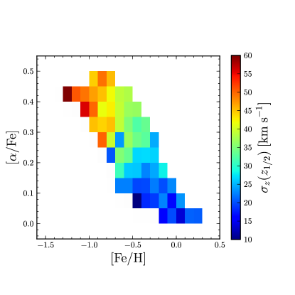
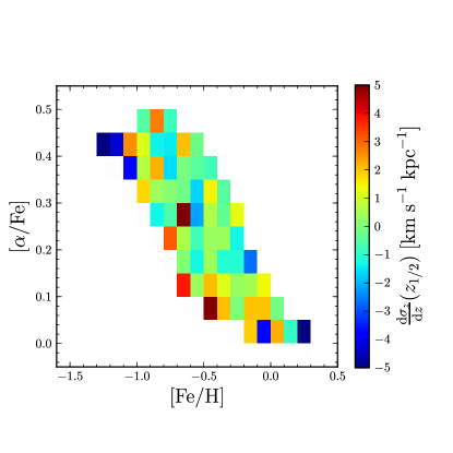
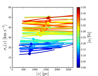
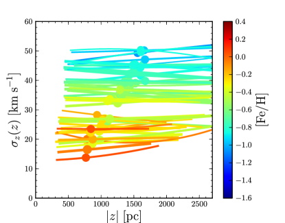
In Figures 2–4 we present the results of our procedure for mapping the vertical velocity dispersion of the SEGUE G-dwarf sample, divided in narrow bins in ($[\mathrm{Fe/H}]$,$[\alpha\mathrm{/Fe}]$). As described above, this procedure is robust to outliers and automatically handles the individual uncertainties in the observed vertical velocities. Figure 2 shows the main result of this paper, namely, that the vertical velocity dispersion profiles of mono-abundance populations, $\sigma_{z}(z,R_{0}\,|\,[\alpha\mathrm{/Fe}],[\mathrm{Fe/H}])$, are nearly constant with height $z$ at some $\sigma_{z}([\mathrm{Fe/H}],[\alpha\mathrm{/Fe}])$—i.e., they are isothermal—and that $\sigma_{z}([\mathrm{Fe/H}],[\alpha\mathrm{/Fe}])$ varies distinctly across chemically-selected sub-populations among the different abundance bins. The two bottom panels of Figure 2 show the vertical dispersion profiles, $\sigma_{z}(z,R_{0}\,|\,\vec{p}_{best})$, for each abundance bin with a 20 % or better determination of $\sigma_{z}(z_{1/2})$, where $\vec{p}_{best}$ represents the peak of the PDF for the model parameters, and the color coding reflects $[\alpha\mathrm{/Fe}]$ (left) and $[\mathrm{Fe/H}]$ (right), respectively. The lines are drawn over the central 95 % of the $|z|$-range of stars in each bin, reflecting the abundance-dependent distance distribution in the sample. Remarkably, $\sigma_{z}$ is nearly constant (within a few km s^-1) for all individual $([\mathrm{Fe/H}],[\alpha\mathrm{/Fe}])$ bins, while the $\sigma_{z}$ values vary from 15 km s^-1 to 50 km s^-1 among the bins. That variation in $\sigma_{z}(z_{1/2},R_{0}\,|\,\vec{p}_{best},[\mathrm{Fe/H}],[\alpha\mathrm{/Fe}])$, where $z_{1/2}$ is the median vertical height above the mid-plane for each mono-abundance data sample, is illustrated in the top left panel of Figure 2, showing that the vertical velocity dispersion increases toward higher $[\alpha\mathrm{/Fe}]$ and lower $[\mathrm{Fe/H}]$ in a pattern that is qualitatively very similar to the corresponding scale-height map of mono-abundance components, $h_{z}([\mathrm{Fe/H}],[\alpha\mathrm{/Fe}])$, from B12a. The top right panel shows the linear slope of the $\sigma_{z}(z,R_{0}\,|\,[\mathrm{Fe/H}],[\alpha\mathrm{/Fe}])$ profile, ${\mathrm{d}}\sigma_{z}(z)/{\mathrm{d}}z$ evaluated at $z_{1/2}$. The slopes are typically at the level of 1 to 3 km s^-1 kpc^-1, with no recognizable dependence on $[\alpha\mathrm{/Fe}]$ and $[\mathrm{Fe/H}]$. We return to this remarkable degree of isothermality below.

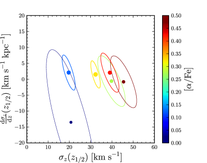
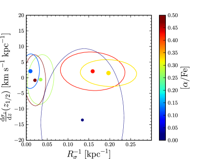
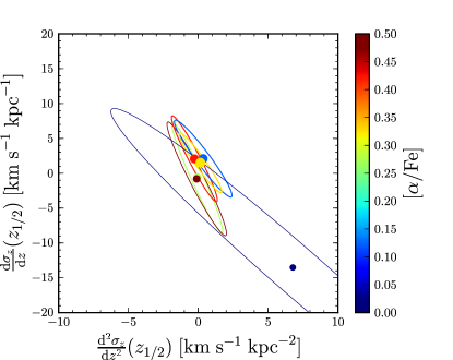
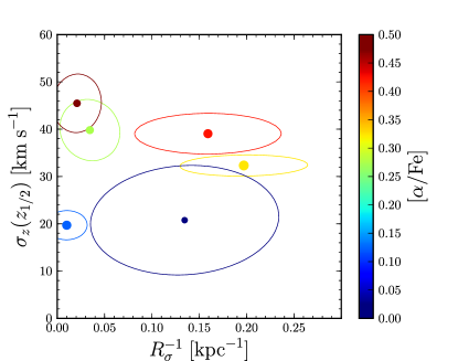
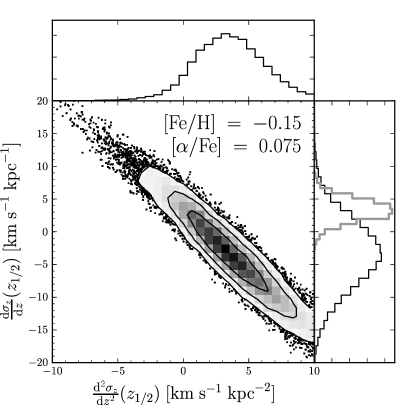
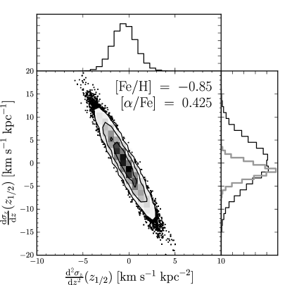
While Figure 2 summarizes the best-fit $\sigma_{z}(z,R_{0}\,|\,[\mathrm{Fe/H}],[\alpha\mathrm{/Fe}])$, Figure 3 illustrates the uncertainties in the inferred parameters $\vec{p}$ for seven representative mono-abundance bins (the uncertainties for the other bins are similar). The PDFs are summarized by the peak and 1-sigma uncertainty ellipses of two-dimensional projections of the full five-dimensional parameter space for each mono-abundance bin. This figure shows that the uncertainty on $\sigma_{z}$ is typically a few km s^-1, such that the slight gap apparent in Figure 2 around $\sigma_{z}=30$ km s^-1 is not significant. This level of uncertainty also does not affect the large abundance-trend of $\sigma_{z}(z_{1/2},R_{0})$ between 10 and 60 km s^-1 in the top panel of Figure 2. Figure 3 also shows that there are no significant correlations among the parameters, except for a slight correlation between the slope and the magnitude of the dispersion and a strong correlation between the slope and quadratic term of the vertical dependence of the velocity dispersion. The slope and quadratic term are anti-correlated, such that the overall change in velocity dispersion over the $|z|$-range of the sample is small in all cases. The parameters of the vertical dependence of $\sigma_{z}$ are not correlated with the inverse scale length $R_{\sigma}$^-1; we discuss the inferred inverse scale length further below. Figure 4 shows the full PDF for the slope and the quadratic term of the vertical dependence of $\sigma_{z}$ for two mono-abundance bins. These full PDFs further illustrate the strong anti-correlation between the slope and quadratic term. This strong anti-correlation does not mean that the data only constrain the vertical slope of the vertical velocity dispersion profile without constraining the second derivative. The fits strongly prefer a flat vertical profile for the velocity dispersion over the full vertical range of $\approx 2$ kpc of the data in each mono-abundance bin.

By combining the individual mono-abundance PDFs for the slope and the quadratic term we obtain a joint estimate for the vertical dependence of the vertical velocity dispersion. The peak of the joint PDF occurs at ${\mathrm{d}}\sigma_{z}(z)/{\mathrm{d}}z=0.7\pm 0.5$ km s^-1 kpc^-1, ${\mathrm{d}}^{2}\sigma_{z}(z)/{\mathrm{d}}z^{2}=-0.12\pm 0.2$ km s^-1 kpc^-2, with strongly correlated error bars. Assuming no quadratic term, the joint estimate for the slope is ${\mathrm{d}}\sigma_{z}(z)/{\mathrm{d}}z=0.3\pm 0.2$ km s^-1 kpc^-1. Thus, each individual mono-abundance bin is consistent with isothermality at the $\sim\!10$ % (few km s^-1) level, and the mean slope is consistent with zero at the percent level (few tenths of a km s^-1), when compared with the range in vertical velocity dispersion present in the full disk sample.

It is hard to judge from Figure 3 whether the individual slope and quadratic term estimates and uncertainties are consistent with the joint estimate, in the sense of these individual estimates really being noisy estimates of the joint estimate. To answer this question, we calculate for each individual mono-abundance (slope and quadratic coefficient) PDF the quantile of the distribution at which the joint estimate lies. In practice, this calculation is done by binning the individual PDF in two dimensions, sorting the binned PDF in ascending order (by flattening the 2D binned PDF into a 1D list), and cumulatively summing the resulting list and normalizing the total sum to one. This list then contains the quantile of the PDF at which each bin in the binned PDF lies, and we can find the bin and quantile corresponding to the jointly estimated slope and quadratic coefficient. We find that the distribution of quantiles thus calculated is relatively flat, with no noticeable dependence on $[\alpha\mathrm{/Fe}]$, indicating that the individual (slope, quadratic coefficient) estimates and uncertainties are consistent with being noisy estimates of the joint slope and quadratic coefficient.

As discussed in $\mathsection$ 2, the distances used could be systematically under- or over-estimated by up to 10 %. Through the dependence on the distance of the velocity component tangential to the line of sight this could lead to a increase or decrease in the velocity dispersion’s vertical gradient. To investigate this we have repeated the analysis while systematically changing the distances by 10 %. We find for both under- and over-estimated distances that the joint estimate for the slope remains consistent with zero, with $\mathrm{d}\sigma_{z}(z)/{\mathrm{d}}z=0.4\pm 0.2$ km s^-1 kpc^-1 and $\mathrm{d}\sigma_{z}(z)/{\mathrm{d}}z=1.1\pm 0.4$ km s^-1 kpc^-1, for distances that are 10 % smaller and larger, respectively. Additionally, we have repeated the analysis considering only stars with $|b|>50^{\circ}$, for which most of the vertical velocity comes from the line-of-sight velocity measurement, which is not affected by distance systematics—and a flat vertical profile remains flat if only the distances change. We find that the inferred vertical profiles are similar to those for the full sample, and the joint estimate for the slope remains consistent with zero: $\mathrm{d}\sigma_{z}(z)/{\mathrm{d}}z=0.0\pm 0.3$ km s^-1 kpc^-1. Keeping only stars with $|b|>60^{\circ}$ gives similar results, but leaves only the metal-poor, $\alpha$-enhanced bins with enough stars do perform the analysis. Thus, we conclude that distance systematics do not influence the inferred isothermality of the mono-abundance populations.

Figure 5.— Variation of the vertical velocity dispersion with Galactocentric radius. Shown is the best-fit inverse radial scale length of the vertical velocity dispersion as a function of $[\mathrm{Fe/H}]$ and $[\alpha\mathrm{/Fe}]$ (left panel) and with error bars as a function of metallicity (right panel). Points in the right panel are color-coded using $[\alpha\mathrm{/Fe}]$ minus the median $[\alpha\mathrm{/Fe}]$ as a function of $[\mathrm{Fe/H}]$. Symbol size is proportional to the square root of the number of data points used in the point’s ($[\mathrm{Fe/H}]$,$[\alpha\mathrm{/Fe}]$) bin. The distribution shown on the vertical axis in the right panel is the joint probability distribution for the (mean) inverse radial velocity-dispersion scale length. The black and gray lines show the mean and standard deviation, respectively, of this distribution; this mean inverse radial dispersion scale length is 0.14$\pm$0.01 kpc^-1 ($R_{\sigma}\approx 7.1$$\pm$0.5 kpc).

4.2. Radial dependence of the vertical dispersion: $\sigma_{z}(R\,|\,[\mathrm{Fe/H}],[\alpha\mathrm{/Fe}])$

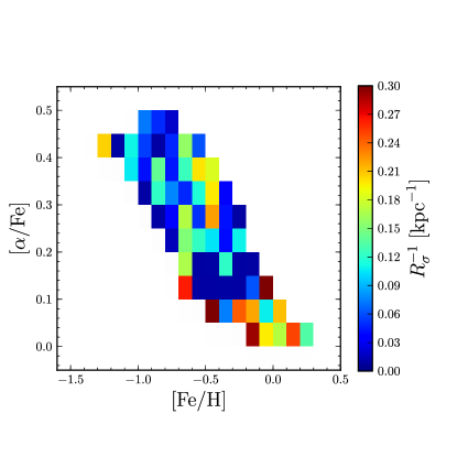
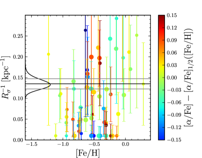
Figure 5 presents the dependence of $\sigma_{z}(z,R\,|\,[\alpha\mathrm{/Fe}],[\mathrm{Fe/H}])$ on Galactocentric radius, where the fit parameter $p_{4}$ from Equation (2) is represented as an inverse scale length, $R_{\sigma}^{-1}$. The left panel shows $R_{\sigma}^{-1}([\mathrm{Fe/H}],[\alpha\mathrm{/Fe}])$. In contrast to $\sigma_{z}([\mathrm{Fe/H}],[\alpha\mathrm{/Fe}])$, there is no discernible systematic dependence of $R_{\sigma}^{-1}$ on $[\mathrm{Fe/H}]$ and $[\alpha\mathrm{/Fe}]$. While $R_{\sigma}^{-1}$ is not well constrained for any individual mono-abundance component, a joint analysis combining all of the individual PDFs for $R_{\sigma}^{-1}$ yields a PDF for $R_{\sigma}^{-1}$ characterized by $0.14\pm 0.01$ kpc^-1, corresponding to a typical outward decrease of $\sigma_{z}(R)\sim\exp\left(-(R-R_{0})/(7.1\pm 0.5~{}\mathrm{kpc})\right)$. This outward decrease of the velocity dispersion, also seen in the luminosity weighted measurements of other disk galaxies, presumably reflects the outward decrease of the disk surface-mass density and its corresponding vertical force. We briefly discuss implications below, but defer dynamical analyses of the vertical kinematics to a separate paper.

As above, we have also checked the influence of distance systematics on the inferred $R_{\sigma}$. Changing the distances by 10 % only has a negligible effect on the inferred $R_{\sigma}^{-1}$. The joint estimate remains $R_{\sigma}^{-1}=0.14\pm 0.01$ kpc^-1 when increasing the distances, and changes within the uncertainties to $R_{\sigma}^{-1}=0.13\pm 0.01$ kpc^-1 when decreasing the distances. We have also repeated the analysis using only stars with $|b|>50^{\circ}$, finding $R_{\sigma}^{-1}=0.16\pm 0.02$ kpc^-1, or $R_{\sigma}=6.4\pm 0.9$ kpc, which is consistent with the estimate using the full sample within the uncertainties.

4.3. The vertical kinematics as a test of the abundance precision

Figure 6.— Impact of abundance errors on the isothermality of the dispersion profile in mono-abundance bins: Three of the panels show the expected slope of $\sigma_{z}(z)$ for different magnitudes of the SEGUE abundance errors, when assuming that each mono-abundance bin is intrinsically isothermal, with velocity dispersions given by the top left panel of Figure 2 and spatial distributions measured by Bovy et al. (2012a, b). The observed slopes are shown in the top right panel. Large abundance errors induce large slopes by ‘mixing’ populations of different $\sigma_{z}$ with proportions that change strongly as a function of $|z|$. This is especially the case in the transition region between the metal-poor, $[\alpha\mathrm{/Fe}]$-enhanced sub-populations and sub-populations with solar abundances. The fact that the observed slopes are $\lesssim$ a few km s^-1 kpc^-1, and that there is no discernible trend in the observed slopes in the transition region, limits the SEGUE abundance errors to be $\delta_{[\mathrm{Fe/H}]}\approx 0.15$ dex and $\delta_{[\alpha\mathrm{/Fe}]}\approx 0.07$ dex (see Figure 7).

Figure 7.— Inferred SEGUE abundance uncertainties, assuming that mono-abundance sub-populations are intrinsically isothermal. The left panel shows the PDF for the abundance uncertainties obtained from comparing the observed slopes with the abundance-error induced slopes (see $\mathsection$ 4.3 and Figure 6); small uncertainties are preferred. The right panel shows the PDF when applying a broad prior centered on the SEGUE-reported abundance uncertainties. The preferred abundance uncertainties are still somewhat smaller than the SEGUE-reported errors. We infer that $\delta_{[\mathrm{Fe/H}]}\approx 0.15$ dex and $\delta_{[\alpha\mathrm{/Fe}]}\approx 0.07$ dex.

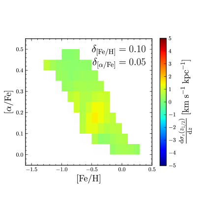
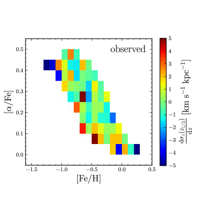
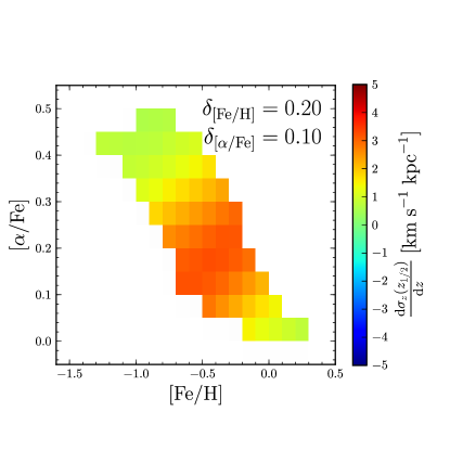
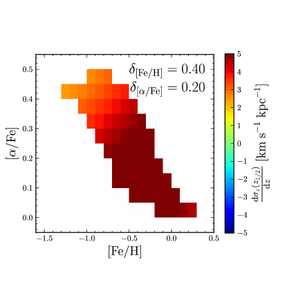
The fact that the data sub-sets we dub ‘mono-abundance components’ exhibit so nearly an isothermal vertical dispersion profile, $|\langle{\mathrm{d}}\sigma_{z}(z_{1/2})/{\mathrm{d}}z([\mathrm{Fe/H}],[\alpha\mathrm{/Fe}])\rangle\lesssim 1$ km s^-1 kpc^-1, while $\sigma_{z}([\mathrm{Fe/H}],[\alpha\mathrm{/Fe}])$ itself varies by nearly 40 km s^-1 among the abundance bins, must set a constraint on how cleanly our ($[\mathrm{Fe/H}]$,$[\alpha\mathrm{/Fe}]$) bins separate abundances, i.e., it allows a completely independent check on the precision (not accuracy) of the SDSS/SEGUE abundance determinations. As the vertical scale heights of these sub-populations vary strongly with abundance (B12a), stars with high $[\alpha\mathrm{/Fe}]$ and low $[\mathrm{Fe/H}]$ will always increase in relative density towards larger $|z|$. As a consequence, a sub-sample selected nominally by its small $[\alpha\mathrm{/Fe}]$ and high $[\mathrm{Fe/H}]$ values will always have far greater ‘contamination’ at large $|z|$ from stars with higher $[\alpha\mathrm{/Fe}]$ and lower $[\mathrm{Fe/H}]$. As those contaminants have a substantially higher $\sigma_{z}$, the dispersion profile should rise away from the mid-plane if such contamination is important. This effect is manifested in samples with poor or no abundance preselection (e.g., Kuijken & Gilmore, 1989; Fuchs et al., 2009).

To turn the observed isothermality of $\sigma_{z}(z\,|\,[\mathrm{Fe/H}],[\alpha\mathrm{/Fe}])$ into a cross-check on SDSS/SEGUE abundances (Lee et al., 2008a, b; Allende Prieto et al., 2008; Lee et al., 2011a), we proceed as follows. We presume that absent any abundance errors, i.e., for the perfect mono-abundance sub-populations, the dispersion profiles would be perfectly isothermal. This toy model for $\sigma_{z}(z)$ is motivated by the fact that the solution for the vertical Jeans equation in cylindrical coordinates with the dominant portion of the disk mass at $|z|<500$ pc (i.e., the limiting case of a mass sheet, with constant vertical force) and an exponential profile for the tracer density (as found in B12a), the solution is $\sigma(z)=$ constant. In this context, any force contribution from a vertically-extended mass distribution (e.g., the halo), will lead to solutions with $\sigma_{z}$ increasing with height, making it unlikely that the error-free dispersion profile slope is negative (i.e., falling with height). We then assume that the observed $\sigma_{z}([\mathrm{Fe/H}],[\alpha\mathrm{/Fe}])$ (top left panel of Figure 2) and $h_{z}([\alpha\mathrm{/Fe}],[\mathrm{Fe/H}])$ (Figure 4 in B12a) are sufficient approximations to the true distribution of these quantities, and we use the normalizations from Bovy et al. (2012b). Viewing then the abundance uncertainties $\delta_{[\alpha\mathrm{/Fe}]}$ and $\delta_{[\mathrm{Fe/H}]}$ as free parameters that correlate bins and hence lead to rising dispersion profiles, we determine for what abundance errors the predicted and observed slopes of the vertical dispersion profile, ${\mathrm{d}}\sigma_{z}(z_{1/2})/{\mathrm{d}}z$, or shorter $\sigma^{\prime}_{z}$, match best. Note that error-induced abundance correlations will not change the dispersion profile slope in all bins, as $\sigma_{z}([\alpha\mathrm{/Fe}],[\mathrm{Fe/H}])$ is a somewhat complex function of $([\mathrm{Fe/H}],[\alpha\mathrm{/Fe}])$. Specifically, we calculate the PDF for $\delta_{[\alpha\mathrm{/Fe}]}$ and $\delta_{[\mathrm{Fe/H}]}$ based on an objective function $\propto\exp\left[-0.5\left(\sigma^{\prime}_{z,obs}-\sigma^{\prime}_{z,mod}(\delta_{[\alpha\mathrm{/Fe}]},\delta_{[\mathrm{Fe/H}]})\right)^{2}/(\sigma_{\sigma^{\prime}_{z,obs}})^{2}\right]$, where $\sigma^{\prime}_{z,mod}(\delta_{[\alpha\mathrm{/Fe}]},\delta_{[\mathrm{Fe/H}]})$ is the dispersion profile slope predicted by the various assumptions on the errors.

Figure 6 shows the abundance-error-induced slopes for a few different magnitudes for the abundance uncertainties and compares these to the observed slopes of Figure 2, repeated as the top right panel in Figure 6. It is clear that the abundance uncertainties can certainly not be much bigger than the SEGUE-reported uncertainties without inducing large slopes and clear patterns in the abundance dependence of the slope.

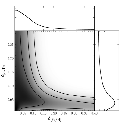
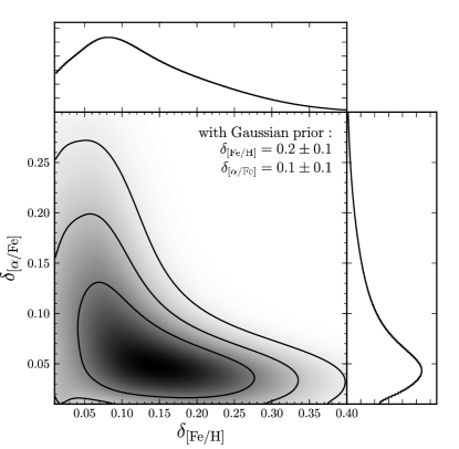
Figure 7 provides the quantitative results of comparing the abundance-errors-induced slopes with the observed slopes. The left panel shows the PDF for $\delta_{[\alpha\mathrm{/Fe}]}$ and $\delta_{[\mathrm{Fe/H}]}$ using flat priors on both, while the right panel shows the PDF assuming Gaussian priors on the error estimates around their nominal value $\delta_{[\alpha\mathrm{/Fe}]}=0.1$ dex (Lee et al., 2011a) and $\delta_{[\mathrm{Fe/H}]}=0.2$ dex (Smolinski et al., 2011), both with a standard deviation of 0.1 dex. The left panel shows that a very clean metallicity separation (i.e., very small $[\mathrm{Fe/H}]$ errors) are suggested by the data. If we include the nominal error priors, we still find that the remarkable near-isothermality of the mono-abundance dispersion profiles implies that the abundance precision are somewhat better than the nominal values, with $\delta_{[\mathrm{Fe/H}]}\approx 0.15$ dex and $\delta_{[\alpha\mathrm{/Fe}]}\approx 0.07$ dex. Note, that this analysis only speaks to the error precision, i.e., the ability to rank stars in their relative abundance, not to the abundance accuracy on any absolute scale.

5. Discussion

5.1. The simplicity of mono-abundance sub-populations

The results in this paper show that the vertical motions of mono-abundance sub-populations of the Milky Way’s disk are extremely simple: they are vertically isothermal to a remarkable degree—we detect no systematic departure from isothermality at the percent level—and declining with radius, in a manner that appears consistent with the decrease in disk surface-mass density (see below). Combined with the findings in B12a that the density of these sub-populations is well described by a single vertical exponential and a single radial exponential, this shows that the phase-space structure of mono-abundance sub-populations is about as simple as it could be. Chemically-homogeneous sub-components of the disk are individually simple disk components that come together to create the complex disk structure that is observed. Typically, this structure has been decomposed—in light of this paper and of Bovy et al. (2012a, b)’s results, perhaps spuriously—into a small number of sub-components with internal metallicity and velocity gradients.

The fact that the mono-abundance sub-populations are so close to vertically isothermal is somewhat surprising, given the inherent complexity in the simple ($[\mathrm{Fe/H}]$,$[\alpha\mathrm{/Fe}]$) abundance plane induced by the (presumably) very different star formation histories in different parts of the disk, and evolutionary processes such as radial migration, which radially mix stars with very different origins. We expect each pixel in the ($[\mathrm{Fe/H}]$,$[\alpha\mathrm{/Fe}]$) abundance plane to contain stars with a variety of ages and birth locations, with only a rough mean-age increase with increasing $[\alpha\mathrm{/Fe}]$. Whether this a-priori reasonable picture is inaccurate, because mono-abundance sub-populations are dominated by a single co-eval population even in the light of star-formation complexity and radial migration, or whether the Milky Way relaxes to this simple state, is a question that is best confronted by more detailed analytic models, simulations or the next generation of spectroscopic surveys that will determine elemental abundances beyond $[\mathrm{Fe/H}]$ and $[\alpha\mathrm{/Fe}]$, such as APOGEE (Eisenstein et al., 2012).

Figure 8.— Vertical temperature distribution of the stellar disk at $\sim\!R_{0}$: Distribution of stellar surface-mass density at the solar radius, $\Sigma_{R_{0}}(\sigma_{z}^{2})$, as a function of vertical velocity dispersion squared, $\sigma_{z}^{2}$. The thick black histogram shows the total stellar surface-mass contributions in bins in $\sigma_{z}^{2}$, calculated by summing the total stellar masses of sub-populations in $[\mathrm{Fe/H}]$ and $[\alpha\mathrm{/Fe}]$. The stellar surface-mass densities of individual abundance bins in $[\mathrm{Fe/H}]$ and $[\alpha\mathrm{/Fe}]$ are shown as dots, calculated by correcting the observed number counts of SEGUE G-type dwarfs into stellar masses using stellar-population-synthesis models as described in Bovy et al. (2012b), with values for $\Sigma_{R_{0}}([\mathrm{Fe/H}],[\alpha\mathrm{/Fe}])$ shown on the $y$-axis. The points are color-coded by the value of $[\alpha\mathrm{/Fe}]$ in each bin and the size of the points is proportional to the square root of the number of data points upon which the kinematic fits are based. The temperature distribution exhibits no evidence for a distinct hot (“thick”) disk component.

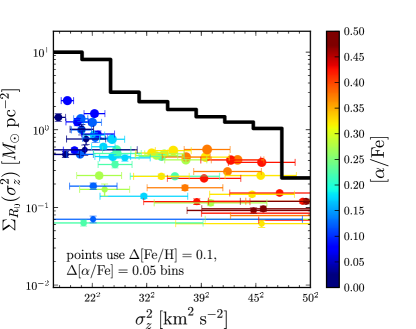
The velocity dispersions of the mono-abundance sub-components increase smoothly from $\sim\!15$ km s^-1 for the $\alpha$-youngest populations to $\gtrsim 50$ km s^-1 for the $\alpha$-oldest. These extrema are typical for thin–thick disk decompositions, but the existence of intermediate populations $\sim\!30$ km s^-1 is unexpected in the traditional picture with a thin–thick disk dichotomy. We apply the procedure of Bovy et al. (2012b) for calculating the total stellar surface-mass density in each mono-abundance bin, correcting the observed number counts for spectroscopic and stellar-population-sampling selection effects using stellar-population-synthesis models (we refer the reader to that paper for more details on this procedure). This stellar mass is not measured dynamically from the vertical kinematics. This results in the stellar surface-mass-weighted distribution of the vertical velocity dispersion or kinetic temperature, shown in Figure 8. Together with Figure 2 in Bovy et al. (2012b), this shows that the distribution of stellar mass in the Milky Way is monotonically, and seemingly continuously, declining from cool, thin-disk components to hotter, thicker disk components, with no gap or bimodality. This, combined with the isothermality of each mono-abundance component, shows that the intermediate populations cannot be a mix of the thinner and thicker components, but that they are real and contribute an amount of stellar mass that is intermediate between the thinner and thicker components as well. This continuity rejects the notion of a dichotomy between a thin and a thick disk in the Milky Way.

We can compare our observational results to some scenarios for creating the thicker disk components, in particular those where a pre-existing thin disk is dynamically heated by an infalling satellite. On this basis, our results reject massive satellite infall as the dominant disk heating mechanism, as such simulations typically display a sharp break in the velocity dispersion between the simulated thin and thick disk (Abadi et al., 2003; Brook et al., 2004; Villalobos & Helmi, 2008), in disagreement with our Figures 2 and 8. This, in addition to the density structure in B12a, points toward an internal mechanism for creating thicker disk components. Such an internal mechanism could be radial migration (Loebman et al., 2011). The thick-disk component could also form internally at early times in a turbulent, clumpy disk (e.g., Bournaud et al., 2009; Förster Schreiber et al., 2009), although creating the continuous distribution of vertical temperatures requires that the disk remains turbulent over a significant fraction of its history (e.g., Forbes et al., 2011). Whether multiple minor satellite mergers can plausibly lead to the continuous trends with elemental abundance of the spatial and kinematic structure in the Milky Way’s disk remains to be seen.

5.2. The radial dispersion profile and dynamical modeling

In the simplest model of a razor-thin disk and an exponential tracer density, solution of the vertical Jeans equation yields the disk surface-mass density, $\Sigma(R)$, in terms of the vertical velocity dispersion $\sigma_{z}$ and the vertical scale height $h_{z}$ of the tracer population: $\Sigma(R)\propto\sigma_{z}^{2}/h_{z}$. Assuming that the tracer’s density does not flare, this implies that the mass scale length of the disk is equal to half of the exponential scale length of the velocity dispersion, and that the dispersion scale length has no abundance dependence. We indeed do not observe any abundance dependence in the inferred $R_{\sigma}^{-1}$ in Figure 5, and B12a found no evidence for a flare in the tracers’ density profile. Thus, we obtain an estimate of the disk’s mass scale length of $\approx 3.5$ kpc from our combined estimated of the dispersion scale length of $R_{\sigma}=7.1\pm 0.5$ kpc. The addition of the dark matter halo, which locally has an equivalent exponential scale length $\gtrsim 5$ kpc, means that this is likely an overestimate, such that we expect the scale length to be $\lesssim 3.5$ kpc.

Rather than trying to estimate the halo correction to the disk scale length as estimated above, we defer a proper dynamical analysis to a separate paper. The simplicity of the mono-abundance sub-populations makes them excellent tracers of the local vertical potential, because their spatial and kinematic simplicity indicates that their phase-space distribution function is simple. This removes the common difficulty in modeling and marginalizing over the phase-space distribution of a kinematic tracer sample when doing dynamical inference (e.g., Bovy et al., 2010). The large number of independent mono-abundance sub-populations that all trace the same underlying gravitational potential will permit for extensive cross-checks. The abundance independence of the inferred dispersion scale length in this paper is a first example of this, and indicates how fruitful such an approach may be.

6. Summary

This paper obtains the following results:

$\bullet$ We modeled the vertical velocity dispersion, $\sigma_{z}(z,R)$, and its spatial dependence of mono-abundance ($[\mathrm{Fe/H}]$,$[\alpha\mathrm{/Fe}]$) slices of the SEGUE G-dwarf sample. We found that all mono-abundance components exhibit nearly isothermal kinematics in the vertical direction, and a slow outward decrease in the radial direction:

$$\sigma_{z}\bigl{(}z,R\,|\,[\alpha\mathrm{/Fe}],[\mathrm{Fe/H}]\bigr{)}\approx\sigma_{z}\bigl{(}[\alpha\mathrm{/Fe}],[\mathrm{Fe/H}]\bigr{)}$$

$$\qquad\qquad\qquad\qquad\qquad\qquad\times\exp\bigl{(}-(R-R_{0})/7\,\mathrm{kpc}\bigr{)}\,.$$

Each mono-abundance component is isothermal to within about 3 km s^-1 kpc^-1. The mean vertical $\sigma_{z}$ gradient is only $0.3\pm 0.2$ km s^-1 kpc^-1, such that the mono-abundance populations are consistent with isothermality at the level of 1 %, when compared to the range of velocity dispersions present in this sample.

$\bullet$ We find a smooth variation in characteristic velocity dispersion from $\sim\!15$ km s^-1 for chemically-young stars with solar abundances to $\gtrsim 50$ km s^-1 for metal-poor, $[\alpha\mathrm{/Fe}]$-enhanced stars that are presumably old. The mass-weighted distribution of vertical kinetic temperatures ($\propto\sigma_{z}^{2}$) is a continuous and monotonically-declining function, similar to the mass-weighted distribution of scale heights found in Bovy et al. (2012b). This, and in particular the existence of isothermal, intermediate-dispersion ($\sim\!30$ to 40 km s^-1) sub-populations, shows that the mono-abundance sub-populations cannot be the mix of a thin, cool disk component and a thick, hotter component. The data therefore reject the notion of a thin–thick-disk dichotomy.

$\bullet$ The remarkable degree of isothermality of the mono-abundance components also allows us to independently verify the SEGUE abundance precision, as it limits the range of abundances actually present within a bin: we find that $\delta_{[\alpha\mathrm{/Fe}]}\approx 0.07$ dex and $\delta_{[\mathrm{Fe/H}]}\approx 0.15$ dex.

$\bullet$ The radial dependence of the vertical velocity dispersion can be described by an exponential. The exponential scale length of this radial dispersion profile has no obvious abundance dependence, as expected when a massive disk contributes significantly to the gravitational potential. The exponential decline of $\sigma_{z}^{2}$ presumably traces the radial decline of the disk’s surface-mass density, but the quality of the data demands careful dynamical modeling beyond the scope of this paper. The simplicity of the vertical phase-space structure of the mono-abundance sub-populations will allow detailed dynamical modeling of the Milky Way’s potential near the disk plane.

References

- Abadi et al. (2003) Abadi, M. G., Navarro, J. F., Steinmetz, M., & Eke, V. R., 2003, ApJ, 591, 499
- Abazajian et al. (2009) Abazajian, K. N., Adelman-McCarthy, J. K., Agũeros, M. A., et al. 2009, ApJS, 182, 543
- Allende Prieto et al. (2008) Allende Prieto, C., Sivarani, T., Beers, T. C., et al. 2008, AJ, 136, 2070
- Bensby et al. (2003) Bensby, T., Feltzing, S., & Lundström, I. 2003, A&A, 410, 527
- Bond et al. (2010) Bond, N., Ivezić, Ž., Sesar, B., et al. 2010, ApJ, 716, 1
- Bournaud et al. (2009) Bournaud, F., Elmegreen, B. G., & Martig, M. 2009, ApJ, 707, L1
- Bovy et al. (2009) Bovy, J., Hogg, D. W., & Rix, H.-W. 2009, ApJ, 704, 1704
- Bovy et al. (2010) Bovy, J., Murray, I., & Hogg, D. W. 2010, ApJ, 711, 1157
- Bovy et al. (2012b) Bovy, J., Rix, H.-W., Hogg, D. W., et al. 2012b, ApJ, 751, 131
- Bovy et al. (2012a) Bovy, J., Rix, H.-W., Liu, C., et al. 2012a, ApJ, 753, 148
- Brook et al. (2004) Brook, C. B., Kawata, D., Gibson, B. K., & Freeman, K. C., ApJ, 612, 894
- Chen et al. (2001) Chen, B., Stoughton, C., Smith, J. A., et al. 2001, ApJ, 553, 184
- Chiba & Beers (2000) Chiba, M. & Beers, T. C. 2000, AJ, 119, 2843
- Eisenstein et al. (2012) Eisenstein, D. J., Weinberg, D. H., Agol, E., et al. 2012, AJ, 142, 72
- Feltzing et al. (2003) Feltzing, S., Bensby, T., & Lundström, I. 2003, A&A, 397, 1
- Flynn & Fuchs (1994) Flynn, C. & Fuchs, B. 1994, MNRAS, 270, 471
- Forbes et al. (2011) Forbes, J., Krumholz, M., & Burkert, A. 2012, ApJ, 754, 48
- Foreman-Mackey et al. (2012) Foreman-Mackey, D., Hogg, D. W., Lang, D., & Goodman, J. 2012, arXiv:1202.3665v2 [astro-ph.IM]
- Förster Schreiber et al. (2009) Förster Schreiber, N. M., Genzel, R., Bouché, N., et al. 2009, ApJ, 706, 1364
- Fuchs et al. (2009) Fuchs, B., Dettbarn, C., Rix, H.-W., et al. 2009, AJ, 137, 4149
- Fuhrmann (1998) Fuhrmann, K. 1998, A&A, 338, 161
- Goodman & Weare (2010) Goodman, J. & Weare, J., 2010, Comm. App. Math. and Comp. Sci., 5, 65
- Ivezić et al. (2008) Ivezić, Ž., Sesar, B., Juric, M., et al. 2008, ApJ, 684, 287
- Jurić et al. (2008) Jurić, M., Ivezić, Ž., Brooks, A., et al. 2008, ApJ, 673, 864
- Kuijken & Gilmore (1989) Kuijken, K. & Gilmore, G. 1989, MNRAS, 239, 605
- Lee et al. (2011a) Lee, Y. S., Beers, T. C., Allende Prieto, C., et al. 2011a, AJ, 141, 90
- Lee et al. (2011b) Lee, Y. S., Beers, T. C, An, D., et al. 2011b, ApJ, 738, 187
- Lee et al. (2008a) Lee, Y. S., Beers, T. C., Sivarani, T., et al. 2008a, AJ, 136, 2022
- Lee et al. (2008b) Lee, Y. S., Beers, T. C., Sivarani, T., et al. 2008b, AJ, 136, 2050
- Liu & van de Ven (2012) Liu, C. & van de Ven, G. 2012, MNRAS, in press, arXiv:1201.1635
- Loebman et al. (2011) Loebman, S. R., Roškar, R., Debattista, V. P., et al. 2011, ApJ, 737, 8
- Munn et al. (2004) Munn, J. A., Monet, D. G., Levine, S. E., et al. 2004, AJ, 127, 3034
- Nordström et al. (2004) Nordström, B., Mayor, M., Andersen, J., et al. 2004, A&A, 418, 989
- Prochaska et al. (2000) Prochaska, J. X., Naumov, S. O., Carney, B. W., McWilliam, A., & Wolfe, A. M. 2000, AJ, 120, 2513
- Schlesinger et al. (2010) Schlesinger, K. J., Johnson, J. A., Rockosi, C. M., et al. 2010, ApJ, 719, 996
- Schönrich & Binney (2009) Schönrich, R. & Binney, J. J. 2009, MNRAS, 396, 203
- Schönrich et al. (2010) Schönrich, R., Binney, J. J., & Dehnen, W. 2010, MNRAS, 403, 1829
- Smolinski et al. (2011) Smolinski, J. P., Lee, Y. S., Beers, T. C., et al. 2011, AJ, 141, 89
- Villalobos & Helmi (2008) Villalobos, A. & Helmi, A., 2008, MNRAS, 391, 1806
- Yanny et al. (2009) Yanny, B., Rockosi, C., Newberg, H. J., et al. 2009, AJ, 137, 4377