An approximate diagonalization method for large scale Hamiltonians
Abstract
An approximate diagonalization method is proposed that combines exact diagonalization and perturbation expansion to calculate low energy eigenvalues and eigenfunctions of a Hamiltonian. The method involves deriving an effective Hamiltonian for each eigenvalue to be calculated, using perturbation expansion, and extracting the eigenvalue from the diagonalization of the effective Hamiltonian. The size of the effective Hamiltonian can be significantly smaller than that of the original Hamiltonian, hence the diagonalization can be done much faster. We compare the results of our method with those obtained using exact diagonalization and quantum Monte Carlo calculation for random problem instances with up to 128 qubits.
I Introduction
Diagonalization of large Hermitian matrices is a difficult problem in linear algebra, with applications in a variety of disciplines. In quantum mechanics, for example, the energy levels of a quantum system are obtained by diagonalization of the system’s Hamiltonian. Knowing those energy levels is necessary for describing the behavior of the quantum system, e.g., the evolution of a quantum computer consisting of quantum bits (qubits). Calculating the exact energy spectrum of a Hamiltonian with usual numerical computation methods is possible only for up to qubits. For larger systems, the size of the Hilbert space () becomes too large for the current level of available computer memory and speed.
Although it is extremely difficult to calculate the exact spectrum of a multi-qubit system for large , there are ways to calculate an approximate spectrum that shows important features of the exact spectrum reliably over a range of parameters. These methods include Density Matrix Renormalization White93 ; Liang94 ; Exler03 ; Schollwock05 , Lanczos Lanczos50 , and Quantum Monte Carlo calculations Sandvik91 ; Sandvik99 ; Engelhardt06 ; PYoung . Perturbation theory is also an approximate method, that is applicable when the system’s Hamiltonian is close to a simpler Hamiltonian, called the unperturbed Hamiltonian, for which the eigenvalues and eigenfunctions are known or easy to calculate. For example, the unperturbed Hamiltonian can be diagonal in some known basis and the perturbation Hamiltonian can have small off diagonal elements in such a basis. One can perform perturbation expansion in powers of a small parameter, characterizing the off-diagonal terms of the Hamiltonian, to find approximate solutions for the eigenvalues and eigenfunctions of the total Hamiltonian.
A true perturbation expansion provides a Taylor expansion of the energy levels in powers of a small parameter. However, such expansion can become extremely complicated when there are energy level degeneracies in the spectrum of the unperturbed Hamiltonian. Moreover, the perturbation expansion can quickly break down if the energy separations of the unperturbed states are small or when there are anticrossings between the eigenstates in the spectrum. Here, we combine perturbation expansion with exact diagonalization techniques to achieve an effective method for approximate diagonalization. The idea is to separate a subspace, e.g., low energy states of the unperturbed Hamiltonian, from other (high energy) states in the Hilbert space. If the unperturbed Hamiltonian is diagonal, then it might be easy to find its lowest energy states using the structure of the problem. Starting from the original Hamiltonian, we derive an effective Hamiltonian in the subspace using perturbation expansion. Perturbation theory brings into consideration, in the expansion of each term of the effective Hamiltonian, the relevant states that are outside the subspace. If the unperturbed states in the subspace are non-degenerate, then there won’t be a unique effective Hamiltonian that can provide perturbed eigenvalues after the diagonalization. Instead, there will be an effective Hamiltonian for each non-degenerate unperturbed state. Since the calculation involves exact diagonalization of these effective Hamiltonians, the final results are not true Taylor expansions in powers of the small parameter, as in usual perturbation expansion. Yet, perturbation plays an important role in the derivation of these effective Hamiltonians.
II The formalism
To derive the effective Hamiltonians, we adopt the projection operator approach to perturbation theory as discussed by Yao and Shi Yao . Consider the Hamiltonian , in which is the unperturbed Hamiltonian and is the perturbation Hamiltonian. The aim of the perturbation theory is to find the eigenvalues and eigenvectors of , with
| (1) |
assuming that the eigenvalues and eigenvectors of are known.
Consider subspace in the Hilbert space of , consisting of vectors . The subspace can include both degenerate and non-degenerate eigenstates of . We introduce projection operators
| (2) |
Since , , and are diagonal in basis, we have
| (3) |
Let denote an eigenstate of that we are trying to calculate. We write , where and . We multiply both sides of (1), written for the eigenstate , by and , respectively, to get
| (4) |
which can be rewritten as
| (5) |
Here, we have used and . Solving the second equation for , we get
| (6) |
Substituting (6) into the first equation in (5), we find
| (7) |
where is an matrix defined by
| (8) | |||||
with being the unity matrix.
So far, Eq. (7) is exact. What it means is that is an eigenvalue and is an eigenvector of in . Therefore, formally by diagonalizing , one can find and , but no information about other eigenvalues of is obtained. Notice that appears in both (8) and (7), therefore it has to be calculated self-consistently. As we shall see, perturbation theory can help to calculate , order by order.
If is independent of , then all the perturbed eigenvalues and eigenvectors in can be found in a single diagonalization. For a -dependent , on the other hand, only one of the eigenvalues, i.e., , has physical meaning, while all other eigenvalues do not correspond to the correct eigenenergies of the spectrum of . In that case, to calculate each , one has to calculate its corresponding , diagonalize it, and select the right eigenvalue that corresponds to . Note that the states found this way will not be orthogonal to each other. This indeed should be the case because only the original eigenstates in the full Hilbert space are supposed to be orthogonal to each other, hence the projected states may not be orthogonal.
As mentioned earlier, is a function of , which itself has to be calculated via diagonalization of . The calculation becomes tractable using perturbation expansion. Consider the expansion
where, . Substituting into (8), we get
| (9) | |||
Writing , where the superscripts denote the order of perturbation, one can calculate order by order. Because of the projection operator , the operator is not singular and is given by
| (10) |
We now derive analytical formulas for all the elements of up to the forth order perturbation. Defining , where and denote unperturbed states in , and assuming that has only off-diagonal elements in the chosen basis so that , we find
| (11) | |||||
where, and
| (12) |
Notice that for each added order of perturbation, a factor of the form is added to the expansion terms. The small parameter of the expansion, therefore, should be -dependent and have the form:
| (13) |
In our numerical calculations, we found the best agreement with exact diagonalization when expanding the diagonal elements to the forth order of perturbation, but the off-diagonal elements to the second order. This can be understood if one considers only two levels, i.e., . By diagonalizing the reduced Hamiltonian corresponding to the two levels, if the diagonal elements are not the same, a second order off-diagonal element contributes a forth order term to the final eigenvalues, as it gets squared. Therefore to be consistent in the order of perturbation, one should expand the off-diagonal terms to the second order.
Notice that all the energy differences in the denominators are of the form and therefore depend on the unperturbed energy of state . As a result the calculated is dependent, unless all the states in are degenerate (even in that case, the forth order correction will still have -dependence through the second term in the last equation of (11)). As we mentioned before, one cannot obtain all eigenstates by a single diagonalization of . Instead, one has to calculate for each unperturbed eigenstate . The important task then is to select, among all the eigenvalues of , the right eigenvalue that corresponds to state , i.e., the perturbation of . If the perturbed levels do not cross each other, then will be the -th eigenvalue after the diagonalization. In cases when the perturbed states do cross each other, the situation becomes more complicated. One can use the overlap of the new eigenfunctions with the old ones to identify which two correspond to each other.
The accuracy of the calculations depends on the small parameter of the perturbation expansion, . To have an estimate of using (13), let represent the lowest energy level outside the subspace , therefore . This provides an upper bound for the small parameter: . Perturbation expansion, thus becomes more accurate for the lowest energy states for which is smallest. Also, the accuracy of the calculations increases by increasing , i.e., increasing . In principle, there is no limit to the accuracy and therefore no fixed radius of convergence as in the usual perturbation theory. By taking , one can achieve 100% accuracy and an unlimited radius of convergence. In practice, however, is limited by the limitation of the computation time and available memory. By keeping small, the diagonalization can be done very quickly, but at the price of less accurate results. Quite naturally, for , small features of the spectrum that depend on the contribution of the higher energy states, beyond and the states included perturbatively, cannot be reproduced.
III Comparison with exact diagonalization and quantum Monte-Carlo simulation
To test our approximate diagonalization method, we study several Hamiltonians with different sizes and compare our results with those of the exact diagonalization and quantum Monte Carlo simulation. The Hamiltonian we consider is an Ising Hamiltonian in a transverse field of the form
| (14) | |||||
| (15) |
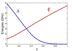
where, , and are dimensionless parameters that can be adjusted, and and are energy scales plotted in Fig. 1. Hamiltonian (14) was studied in Ref. Kamran, to investigate the scaling performance of an adiabatic quantum computation (AQC) Farhi processor based on realistic Hamiltonian parameters. In that case, represents normalized time, where is the total evolution time. It is known Farhi that in AQC, the minimum energy gap between the lowest two energy levels during the evolution determines the time of the computation. Therefore it is important to diagonalize the Hamiltonian (14) to calculate the minimum energy gap. Details of the AQC processor considered in this study are described in other publications Harris10 ; Johnson11 . Here, we only focus on the diagonalization of the Hamiltonians.
In Ref. Kamran, , a number of random Ising instances were generated and the size of the minimum gap in the spectrum of their Hamiltonians was calculated using QMC simulation. With QMC simulation, one can calculate the energy gap between the lowest two energy levels using the method discussed in Kamran ; PYoung . The instances used in Ref. Kamran, were generated by choosing uniform randomly from the set {-1/3,1/3} and a structured set of nonzero values to be either -1, or uniform randomly from {-1/3,1/3}. The connectivity of the graph considered was motivated by a realistic quantum annealing processor as described in Johnson11 ; Kamran . Here, we use the same set of problems and compare our results with the QMC results of Ref. Kamran, .
First, we need to find the unperturbed eigenstates and eigenvalues of for the instances studied. Since is already diagonal, it is only needed to determine the states with the lowest energy to form . For that to be feasible up to 128 qubits, we use the structure of the graph of nonzero couplings between the qubits. We use a dynamic programming method that is a variation on the bucket elimination algorithm Elimination . We select an order in which to “eliminate” the qubits, i.e. to solve for the optimal value of a qubit conditional on the values of all qubits coupled to it that have not yet been eliminated. After eliminating all qubits, the lowest energy state is simply retrieved by tracing back from the optimal value of the qubit that was eliminated last. To find the low energy states, we keep track of the energy increase from choosing the suboptimal value of each qubit being eliminated, and while tracing back through the elimination, the lowest energy partial states encountered so far are kept, instead of just the optimal partial state. With this approach, the ability to find these unperturbed states is primarily limited by the largest number of qubits that need to be simultaneously considered during the elimination (the treewidth of the graph), instead of the total number of qubits. For the instances considered, the treewidth was up to 16.
We choose the unperturbed and perturbation Hamiltonians in the following way:
| (16) |
The small parameter in the perturbation expansion, therefore, is proportional to . In our calculations we kept in the subspace . We choose in such a way that all the degenerate states in the topmost energy level are included in the subspace . A simplifying observation, for the calculation of (11), is that only contains terms with operators of the form which flips the state of qubit in the basis. For each , therefore, only one bit flip from the original state is allowed. Consequently, in the calculation of the matrix elements of effective Hamiltonians , using (11), only states with at most two bit flips from states and participate in the sums. This significantly restricts the states , , or that are summed over in (11). The states outside were found by flipping qubits away from states in , as required by the perturbation expansion.
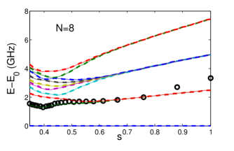
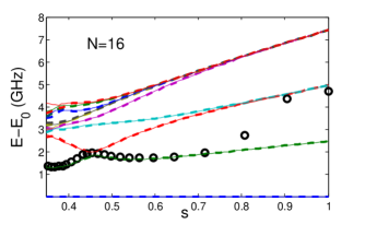
We have examined many instances and compared the calculated approximate eigenvalues with the QMC simulation results of Ref. Kamran and also, for small size instances, with the exact diagonalization results. Here, however, we only report a few sample instances. Figure 2(a) and (b) show the calculated spectra for of 8-qubit and 16-qubit sample problems, respectively. Due to the small number of qubits, the exact diagonalization was possible for these instances. The figures show excellent agreement between the exact (dashed lines) and approximate (solid lines) diagonalization methods over a wide range of the normalized time . Even complicated details of the exact spectra are nicely reproduced by the approximate diagonalization. As expected, some of the higher energy curves deviate from the exact diagonalization values at small , where the perturbation expansion starts to fail. By increasing , one can increase the validity range of the calculation at the expense of a longer computation time. The QMC results (symbols) for the above two instances are also plotted in the same figures. As can be seen, QMC agrees very well with the two other methods for . For larger values of , QMC simulation fails to give reliable results due to the small tunneling amplitudes. As we shall see below, the same pattern continues for larger scale problems.
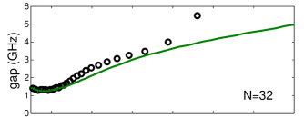
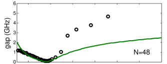
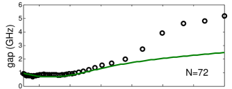
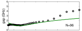
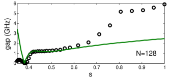
For problems with , it is not feasible to perform exact diagonalization as the size of the Hamiltonian becomes exponentially large. As a consequence, we only compare our results with those calculated using QMC simulations. Figure 3 shows the calculated gap between the lowest two energy levels, for from 32 to 128. For most instances the approximate diagonalization results agree with QMC calculations for . As before, QMC fails to give the correct spectral gap for large . Also, for the values chosen, the perturbation expansion becomes less reliable for , although the accuracy can always be enhanced by increasing . Interesting examples are and 128 for which there are anticrossings in the spectrum. The position of the anticrossing and the shape of the energy levels close to it are more or less consistent between the two methods of calculation. The size of the minimum gap at the anticrossing point, however, can depend on states outside the subspace that are not included in the perturbation calculation. Therefore, the minimum gap size cannot be reliably predicted unless a very large number of states are included in , or alternatively, the perturbation is expanded to high orders.
IV Conclusions
We have developed an approximate diagonalization method for calculating low energy eigenvalues and eigenfunctions of a large scale Hamiltonian. The method is based on derivation of a series of effective Hamiltonians, in a subspace consisting of low energy states of an unperturbed Hamiltonian, using perturbation expansion. For each eigenvalue to be calculated, an effective Hamiltonian is calculated and diagonalized separately. We have applied our method to find the energy eigenvalues of random Ising Hamiltonians in a transverse field. Our results agree very well with the exact diagonalization for 8 and 16 qubit Hamiltonians, and with quantum Monte Carlo simulations for up to 128 qubits. The approximate diagonalization method, however, is extremely faster than both of the above methods.
Acknowledgment
We thank Elena Smirnova and Elena Tolkacheva for critically reading the manuscript and providing valuable comments.
References
- (1) S. R. White, Phys. Rev. B 48, 10345 (1993).
- (2) S. Liang and H. Pang, Phys. Rev. B, 49, 9214 (1994).
- (3) M. Exler, J. Schnack, Phys. Rev. B 67, 094440 (2003).
- (4) U. Schollwöck, Rev. Mod. Phys. 77, 259 (2005).
- (5) C. Lanczos, J. Res. Nat. Bur. Stand. 45, 255 (1950).
- (6) A. W. Sandvik, J. Kurkij arvi, Phys. Rev. B 43, 5950 (1991).
- (7) A. W. Sandvik, Phys. Rev. B 59, R14157 (1999).
- (8) L. Engelhardt, M. Luban, Phys. Rev. B 73, 054430 (2006).
- (9) A. P. Young, S. Knysh, and V. N. Smelyanskiy, Phys. Rev. Lett. 104, 020502 (2010).
- (10) D. Yao and J. Shi, Am. J. Phys. 63, 278 (2000).
- (11) E. Farhi et al., Science, 292, 472 (2001).
- (12) R. Harris et al., Phys. Rev. B 82, 024511 (2010).
- (13) M.W. Johnson et al., Nature 473, 194 (2011).
- (14) K. Karimi, N.G. Dickson, F. Hamze, M.H.S. Amin, M. Drew-Brook, F.A. Chudak, P.I. Bunyk, W.G. Macready, G. Rose, eprint arXiv:1006.4147.
- (15) K. Kask, R. Dechter, J. Larrosa and F. Cozman, “Bucket-Tree Elimination for Automated Reasoning”, ICS Technical Report R92.