Coulomb Glasses: A Comparison Between Mean Field and Monte Carlo Results

Abstract

Recently a local mean field theory for both eqiulibrium and transport properties of the Coulomb glass was proposed [A. Amir et al., Phys. Rev. B 77, 165207 (2008); 80, 245214 (2009)]. We compare the predictions of this theory to the results of dynamic Monte Carlo simulations. In a thermal equilibrium state we compare the density of states and the occupation probabilities. We also study the transition rates between different states and find that the mean field rates used in the aforementioned papers underestimate a certain class of important transitions. We propose modified rates to be used in the mean field approach which take into account correlations at the minimal level in the sense that transitions are only to take place from an occupied to an empty site. We show that this modification accounts for most of the difference between the mean field and Monte Carlo rates. The linear response conductance is shown to exhibit the Efros-Shklovskii behavior in both the mean field and Monte Carlo approaches, but the local mean field method strongly underestimates the current at low temperatures. When using the modified rates better agreement is achieved.

I Introduction

Electronic states in disordered materials can be localized and at zero temperature the material can be insulating. At finite temperature, transport can still occur trough hopping between the localized stated. The energy mismatch between the states must be supplied by emission or absorption of phonons, so the process is called phonon-assisted hopping. This has been studied for many years, one of the early major developments being Mott’s concept of variable range hoppingMott (1968) (VRH) leading to the Mott law for the temperature dependence of the conductivity:

$$\sigma\propto\exp[-(\tilde{T}_{0}/T)^{1/(d+1)}]\,.$$ (1)

Here $T$ is temperature, $\tilde{T}_{0}$ is some constant dependent on the material parameters while $d$ is the dimensionality of the conduction problem. Mott gave only a heuristic derivation of this law based on the idea of a competition between tunneling distance and energy difference. This was later rigorously derived using percolation arguments.Ambegaokar et al. (1971); Shklovskii and Efros (1971); Pollak (1972); Shklovskii (1972) This puts the theory on a firm basis but it applies only in the case of non-interacting electrons. If Coulomb interactions are important, the theory has to be extended. The first step in this direction was the understanding of the interaction-induced dip in the density of states (DOS).Pollak (1970, 1971); Srinivasan (1971) Based on a stability argument on states which are stable to all one-particle jumps, Efros and ShklovskiiEfros and Shklovskii (1975) derived an upper bound on the density of states increasing as $\epsilon^{d-1}$ where the excitation energy $\epsilon$ is counted from the Fermi level. At finite temperatures the gap is smeared by thermal fluctuations.Pikus and Efros (1994)

While the arguments up to this point seem rigorous, one then proceeds with some type of mean field (MF) treatment.Shklovskii and Efros (1984) Since the energy of a certain site depends on the occupancy of the other sites through the Coulomb interaction, the site energies will fluctuate in time as jumps take place. Instead of following the fluctuatig occupation numbers, one replaces them with some average occupancy of each site. In this way, one can repeat Mott’s argument replacing the uniform density of states with the Coulomb gap form, leading to the Efros-Shklovskii (ES) law for conductivity:Efros and Shklovskii (1975)

$$\sigma\propto\exp[-(T_{0}/T)^{1/2}]\,.$$ (2)

While this law has been seen in many experiments, it is difficult to prove rigorously that a manifestly many-particle concept like the Coulomb gap density of states can be used in a single particle picture like that given by Mott.

Recently there was renewed interest in these questions, and local mean field (LMF) theory was revisitedAmir et al. (2008) and applied to time-dependent phenomena, see Refs. Amir et al., 2011; *AmirPNAS for reviews. Having been applied to the VRH problemAmir et al. (2009) the LMF theory has reproduced the ES temperature dependence (2) of the conductance. The LMF approach differs form the conventional one, Shklovskii and Efros (1984) which we refer to as ESMF, by two aspects. Firstly, the LMF equations solved numerically at finite temperature are intended to represent equilibrium state and therefore to allow for the finite-temperature smearing of the Coulomb gap. Contrary, the ESMF approach uses the ground state as a starting point and allows for finite temperatures only in the occupation numbers. Secondly, the LMF uses a different expression for the transition rate between the states, which neglects Coulomb correlations in the transferred energy that seems to be inconsistent. This issue will be discussed in detail in Sec. II. Because of that, the LMF approach is still beyond full control, and there are still questions about its validity. It is therefore important to check the results, see if they can be trusted in some regions of parameters and in this way obtain limits of the validity of the mean field approximation. In this work we compare the MF analysis to dynamic Monte Carlo simulations of the hopping process. This allows us to compare both equilibrium properties like the DOS and the occupation numbers, as well as dynamical aspects like the transition rates and the conductance.

We will conclude that the LMF strongly underestimates the rate of a certain important class of transitions, and this leads to an underestimation of the current. We propose a modification of the transition rates entering the mean-filed scheme in the spirit of the considerations of Ref. Shklovskii and Efros, 1984, Secs. 10.1.2 and 10.2.1 (see also Refs. Levin et al., 1982a; *levin82a), which takes into account the interaction-induced correlations at the minimal level, and ensures that a transition will take place only from an occupied to an empty site. This gives much better estimates for the transition rates, and better agreement with the Monte Carlo simulations of the conductance.

Note that recently the question of a finite temperature phase transition to a low temperature glass phase was discussed, and it was found that mean field theories Pastor and Dobrosavljevic (1999); *vojta93; *muller04; *muller07; *pankov05 predict such a phase transition while this was not found in Monte Carlo simulations.Surer et al. (2009); Goethe and Palassini (2009)

The paper is organized as follows. In Sec. II we recall the MF approach and explain our modified transition rates. In Sec. III we outline the numerical Monte Carlo method we use to test the MF results. We comparw the properties (DOS and occupation probabilities) of equilibrium states in Sec. IV. The transition rates are compared in Sec. V and the conductance in Sec. VI. In Sec. VII we summarize the results.

II Mean field equations

In Ref. Amir et al., 2008, a LMF approach was developed and then applied to the calculation of the conductivity in the variable range hopping regime.Amir et al. (2009) We give here a brief summary of their method. We model the system as a set of sites, each of which can be either empty or occupied by one electron. For numerical convenience, the sites are arranged in a two dimensional square lattice with lattice constand $d$. Each site is given an energy $\phi_{i}$ uniformly distributed in the interval $[-U,U]$. The total single-particle (addition or subtraction) energy (SPE) of site $i$ is then

$$\epsilon_{i}=\phi_{i}+\sum_{j\neq i}\frac{n_{j}-\nu}{r_{ij}}\,.$$ (3)

Here distances $r_{ij}$ between sites $i$ and $j$ are measured in units of $d$ while energies are measured in units of $e^{2}/d$ where $e$ is the electronic charge. Background dielectric constant $\kappa$ is set to 1. $n_{j}=0,1$ is the occupancy of site $j$. The compensating background charge $\nu$ measured in unites of $e$ and associated to each site is introduced to keep the system neutral. We have considered the case of half filling, so that the number of electrons is half the number of sites, and therefore $\nu=1/2$. The occupation numbers $n_{i}$, and therefore also the energies $\epsilon_{i}$, fluctuate in time as the electrons jump between the sites. In the MF approximation, one replaces the fluctuating quantities by their averages, associating to each site an average occupancy $f_{i}=\langle n_{i}\rangle$ and average energy

$$E_{i}=\langle\epsilon_{i}\rangle=\phi_{i}+\sum_{j\neq i}\frac{f_{j}-\nu}{r_{ij}}\,.$$ (4)

The average occupancy is postulated to be given by the Fermi distribution at the average energy,

$$f_{i}=f_{\text{FD}}(E_{i})\equiv\left(e^{E_{i}/T}+1\right)^{-1}.$$ (5)

Equations (4) and (5) form a closed set, which we call the mean field equations. It has been shownAmir et al. (2009) that the solutions of these equations give a density of states with a linear (in 2 dimensions) gap at the Fermi level as expected from the analysis of the Coulomb gap by the stability condition in the ground state.Shklovskii and Efros (1984)

To calculate the conductance we must consider the transition rates between the different sites. If an electron hops from site $i$ to site $j$ the change in the systems energy is

$$\Delta\epsilon_{ij}=\epsilon_{j}-\epsilon_{i}-1/r_{ij}\,.$$ (6)

Here the final term arises because in the definition of $\epsilon_{j}$ it was assumed that site $i$ was initially occupied and site $j$ was initially empty. Therefore the hopping event creates an electron on site $j$ and a hole on site $i$, which attract each other with the energy $r_{ij}^{-1}$. The energy change $\Delta\epsilon_{ij}$ must be supplied by the emission or absorption of a phonon. The rate of such a process is given byShklovskii and Efros (1984)

$$\Gamma_{ij}=\tau_{0}^{-1}(|\Delta\epsilon_{ij}|/E_{0})e^{-2r_{ij}/a}|N(\Delta\epsilon_{ij})|n_{i}(1-n_{j})$$ (7)

where $E_{0}$ is some energy scale characteristic of the electron-phonon interaction (we set it to 1 in the following), $\tau_{0}$ is a microscopic timescale which we take as our unit of time, $a$ is the localization length, which we set equal to the lattice constant $d$, and $N(E)=1/(e^{E/T}-1)$ is the Planck function. The difference $\Delta\epsilon_{ij}>0$ corresponds to phonon absorption, while $\Delta\epsilon_{ij}<0$ corresponds to phonon emission. In this case, $|N(\Delta\epsilon_{ij})|=N(|\Delta\epsilon_{ij}|)+1$ allowing for spontaneous emission.

In the mean field approximation the product $|N(\Delta\epsilon_{ij})|n_{i}(1-n_{j})$ is replaced by its ensemble average, $\langle|N(\Delta\epsilon_{ij})|n_{i}(1-n_{j})\rangle$, which is then decopled into a product of averages, $|N(\langle\Delta\epsilon_{ij}\rangle)|f_{i}(1-f_{j})$. As a result, the rates $\Gamma_{ij}$ are replaced by

$$\gamma_{ij}=\frac{1}{\tau_{0}}\frac{|\langle\Delta\epsilon_{ij}\rangle|}{E_{0}}e^{-2r_{ij}/a}|N(\langle\Delta\epsilon_{ij}\rangle)|f_{i}(1-f_{j}).$$ (8)

In Ref. Amir et al., 2009 it was argued that the energy change should be taken as the difference in the average energies without including the last term in Eq. (6),

$$\langle\Delta\epsilon_{ij}\rangle=E_{j}-E_{i}\,.$$ (9)

The formal reason for omitting the self-interaction term is that it is necessary in order to have detailed balance in equilibrium, $\gamma_{ij}^{0}=\gamma_{ji}^{0}$ where the superscript 0 indicates that these are the rates in equilibrium in the absence of an applied electric field. It is also argued that this is natural in a mean field approach since charge can be thought of as transferred continuously and this term is proportional to the transferred charge squared which is then infinitesimal.

The above considerations seem worrying for two (closely related) reasons. First, the energies of the phonons must be calculated including this term, so it appears that the mean field approach will give an incorrect energy balance between the electrons and the phonon bath. Second, there will be a number of transitions which are given a mean field rate very different (and much smaller) than the real rate. To see this point clearly, consider the situation where $E_{i}<0$ and $E_{j}>0$ while both $|E_{i}|\gg T$ and $|E_{j}|\gg T$. Then $f_{i}\approx 1$ and $f_{j}\approx 0$. This means that it will often be the case that site $i$ is occupied and site $j$ empty. This is a necessary condition for the transition from site $i$ to site $j$ take place, and the fact that it is likely to happen is reflected in the fact that in (8) the factor $f_{i}(1-f_{j})\approx 1$. But $E_{j}-E_{i}$ is positive and larger than temperature so that the rate is strongly suppressed by the factor $N(|\langle\Delta\epsilon_{ij}\rangle|)\approx e^{-(E_{j}-E_{i})/T}$. The real energy change if the transition is from a configuration where site $i$ is occupied and site $j$ empty and where the single particle energies $\epsilon_{i}$ and $\epsilon_{j}$ are close to the averages $E_{i}$ and $E_{j}$ is given by Eq. (6). If the sites are so close that $\epsilon_{j}-\epsilon_{i}<r_{ij}^{-1}$ the process will be an emission process rather than an absorption process, and $N(|\Delta\epsilon_{ij}|)\approx 1$ so the transition rate is exponentially larger than what is found using the approximation (9).

It appears that for the considered configuration the approximation (9) is not a good one and misses an important physical property of the process. To improve this while keeping the microscopic balance we propose the following. We keep the mean field equations (4) and (5) for calculating the average occupation numbers $f_{i}$. But when calculating the rate $\gamma_{ij}$ we consider the joint occupation probabilities for both sites. This follows closely the reasoning of Ref. Shklovskii and Efros, 1984 (Sec 10.1.2) except that there all other sites were considered to be in the ground state configuration, whereas here we assume them to have the mean field average occupation.

Let $F(n_{i},n_{j})$ denote the probability to find the system with occupation numbers $n_{i}$and $n_{j}$, all other sites having the mean field occupation $f_{k}$. $F(n_{i},n_{j})$ depends on the energy changes when adding particles to the sites $i$ and $j$. We define

$$E_{i(j)}=\phi_{i}+\sum_{k\neq i,j}\frac{f_{k}}{r_{ik}}$$ (10)

as the energy of site $j$ not taking into account the interaction with site $j$ (note that here we are omitting the background charge $\nu$ since it will cancel from all energy differences). Starting from the state where both the sites are empty, the energy changes to the other states are

$$E(n_{i},n_{j})=E_{i(j)}n_{i}+E_{j(i)}n_{j}+n_{i}n_{j}/r_{ij}.$$ (11)

We then get

$$F(n_{i},n_{j})=Z_{ij}^{-1}e^{-E(n_{i},n_{j})/T}$$ (12)

where

$$Z_{ij}=1+e^{-E_{i(j)}/T}+e^{-E_{j(i)}/T}+e^{-(E_{i(j)}+E_{j(i)}+1/r_{ij})/T}$$

is the partition function. The transition rate is then

$$\gamma_{ij}=\frac{1}{\tau_{0}}\frac{|\Delta E_{i(j)}|}{E_{0}}e^{-2r_{ij}/a}|N(\Delta E_{i(j)})|F(1,0)\,.$$ (13)

These rates satisfy the detailed balance condition $\gamma_{ij}^{0}=\gamma_{ji}^{0}$ in the absence of an applied electric field and they properly take into account the energy change in the transition. Equation (13) plus a LMF scheme takes into account both the intra-site and inter-site correlations at the minimal level of ensuring that jumps only take place from occupied to empty sites and the finite temperature modification of the ground state. We refer to this theory as the modified local mean field (MLMF) theory. In the following we will compare this to Monte Carlo simulations.

III Numerical algorithm

We used the kinetic Monte Carlo algorithm introduced in Refs. Tsigankov and Efros, 2002; Tsigankov et al., 2003. It consists in writing the rate (7) as a product of a distance dependent part, $\Gamma^{D}_{ij}\equiv e^{-2r_{ij}/a}$, and an energy dependent part,

$$\Gamma^{E}_{ij}\equiv\tau_{0}^{-1}(|\Delta\epsilon_{ij}|/E_{0})|N(\Delta\epsilon_{ij})|n_{i}(1-n_{j})\,.$$

$\Gamma^{D}$ is independent of the configuration and can be precalculated and stored. Since we are working on a lattice, it depends only on the relative distance, and this is not too costly. The program first selects an electron at random and then a possible jump weighted by the rates $\Gamma^{D}$. If the final site is empty, the jump is then accepted with probability $\Gamma^{E}$. Because of the linear dependence of $\Gamma^{E}$ on $|\Delta\epsilon_{ij}|$ it is unbounded for large negative $\Delta\epsilon_{ij}$. For this reason, the rate has to be limited by some maximal rate, which we have taken rather arbitrarily as $3T$ where $T$ is the temperature and the rates then normalized so that the maximal rate has probability 1 for being accepted. We have checked that the exact value of the maximal rate is not important as long as we are not applying strong electric fields,Voje (2009) far beyond the linear response we will consider below.

IV Equilibrium states

Figure 1: The density of states of SPEs at four temperatures: Solid lines: Averaged Monte Carlo simulations. Dashed lines: Averaged mean field solutions. For Monte Carlo simulations: Averaging were done over one ($T=0.1$), three ($T=0.04$ ), six ($T=0.02$) and six ($T=0.01$) Monte Carlo simulations;. Mean field solutions were averaged over 100 solutions for each temperature.

We can now compare several properties of the equilibrium states as described by the LMF and Monte Carlo methods. In all comparisons we use the same sample for both methods, so that we are certain that all differences are a result of the approximations of the mean field model. We use a sample of size $100\times 100$ sites and an on-site disorder $U=1$. In the Monte Carlo simulations we average over from 1 to 6 initial configurations (at high temperatures, thermal motion is sufficient to wash out any difference between initial states). From each initial state we perform $3\cdot 10^{6}$ jumps to equilibrate the system and then we average over the next $5\cdot 10^{5}$ jumps. We solve the mean field equations numerically by an iterative procedure. The presented results are averages over 100 different solutions of the mean field equations.

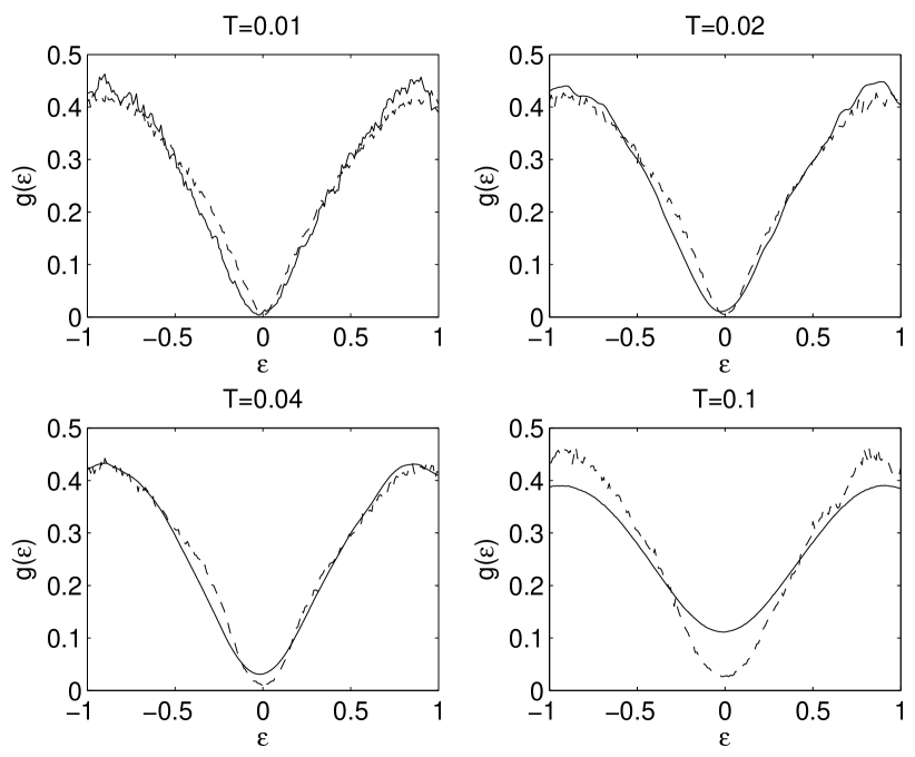
Let us first study the density of single particle states ($\epsilon_{i}$ in the Monte Carlo simulations $E_{i}$ in the mean field solutions). At low temperatures this should display the Coulomb gap, which according to the stability analysis of one-particle stable states should be linear in two dimensions.Shklovskii and Efros (1984) It was previously shownGlatz et al. (2008) that in one-particle stable states with $U=1$ we get in two dimensions a Coulomb gap which is not fully linear but rather of the form $\propto|\epsilon|^{1.2}$. With the accuracy that we are working here we do not expect to see the departure from linear. For the thermal equilibrium states the corresponding quadratic law in three dimensions was confirmed.Goethe and Palassini (2009) The mean field equations was previously shown to give a linear Coulomb gapAmir et al. (2008) at low temperatures. Here we compare the solutions of the LMF equations to Monte Carlo results at different temperatures (Fig. 1).

At low temperatures we see that the two methods give similar results and close to the expected linear Coulomb gap. At higher temperatures the Coulomb gap is smeared by thermal fluctuations. We observe that the smearing is much more efficient in the Monte Carlo simulations than in the mean field solutions. Thus, the mean field equations underestimate the smearing of the Coulomb gap at finite temperatures. This can also be illustrated by plotting the density of states at the Fermi level, $g(0)$, as function of temperature (Fig. 2).

Figure 2: Density of states at the Fermi level, $g(0)$. The mean field results are the averages over 100 ($U=1$) and 50 ($U=5$) solutions. Graphs show a near linear dependence on temperature for mean field equations, while Monte Carlo solutions are near linear at higher temperatures, while showing non-linear behavior at low temperatures.

In the LMF $g(0)$ is close to a linear function, $g(0)=\alpha T$. For the Monte Carlo we find that the dependence is slightly superlinear, but if fitted by a linear function we get a slope of $\alpha=1.54$ in reasonable agreement with the previous results,Levin et al. (1987) which gave $\alpha=1.3$. For the mean field we get $\alpha=0.25$, which is almost twice the result of Ref. Amir et al., 2008 where it was found that $\alpha=0.15$. Note however that in that work sites were at random. In addition, the line does not pass through the origin as it should, and therefore we do not believe that their result is numerically accurate. It used $U=5$, but we have confirmed that we get the same results in that case so this is not the source of discrepancy.

A self consistent equation for the energy dependence of the density of statesMogilyanskii and Raikh (1989) predicts the scaling law (in our units)

$$g(\epsilon,T)=T\mathcal{F}_{2}\left(\epsilon/T\right)\,.$$

We find that our LMF results are compatible with this equation. However, the results of the Monte Carlo simulations do not collapse to this law. This is also evident from the superlinear temperature dependence shown in Fig. 2.

We can also compare the occupation numbers $f_{i}$ with the time averaged occupation numbers $\langle n_{i}\rangle$ in the Monte Carlo simulations. Figure 3 shows the fraction of sites which have a certain value of $|f_{i}-0.5|$ or $|\langle n_{i}\rangle-0.5|$.

Figure 3: Fraction of sites with intermediate occupation. Empty symbols: Mean field solution averaged over 100 solutions for each temperature. Filled symbols: Monte Carlo $\langle n_{i}\rangle$ averaged over $5\cdot 10^{5}$ jumps.

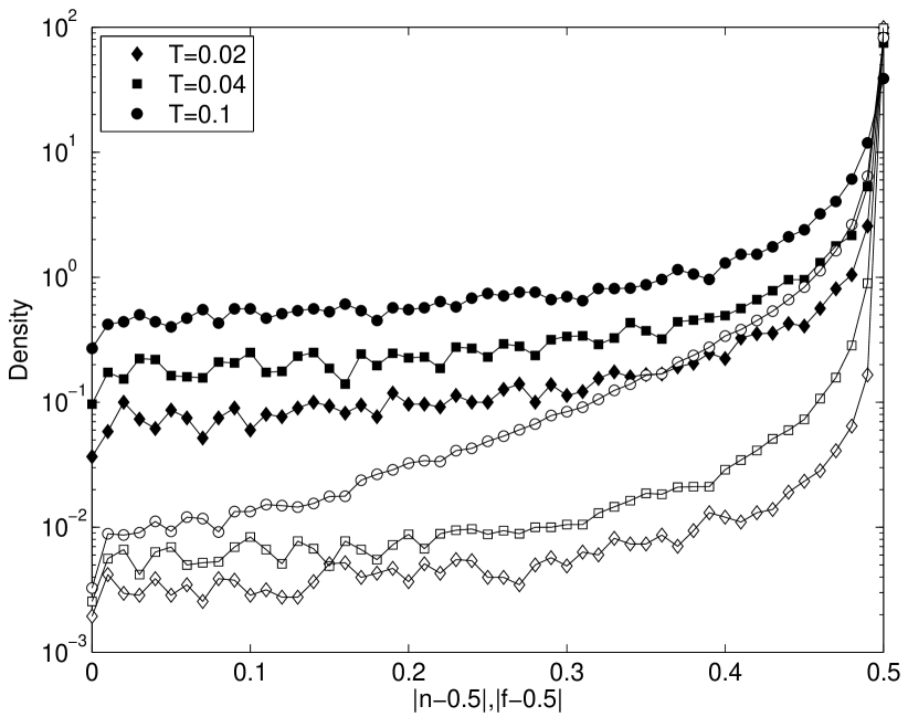
It is clear that the mean field equations underestimate the number of sites with intermediate occupation numbers.

V Transition rates

We can compare the transition rates calculated using the different models. In the Monte Carlo simulations we simply count how often a transition takes place from a site of energy $E=\epsilon_{i}$ to a site of energy $E^{\prime}=\epsilon_{j}$. That is, we refer to the energies before the transition took place. The change in energy is then $\Delta\epsilon=\epsilon_{j}-\epsilon_{i}-1/r_{ij}$.

In the mean field calculations we have to take some care in associating the proper energies to a transition so that comparison to the Monte Carlo results is meaningful. The solution of the mean field equations provides a set of occupation numbers $\{f_{i}\}$ and energies $\{E_{i}\}$. The energy of site $i$ before the transition is given by $E=E_{i(j)}=E_{i}-f_{j}/r_{ij}$ since this is the energy assuming site $j$ to be empty. The energy of site $j$ before the transition is $E^{\prime}=E_{j(i)}+1/r_{ij}=E_{j}+(1-f_{i})/r_{ij}$ since we know that before the transition site $i$ is occupied. In Fig. 4 we show the average of the sum of the rates from energy $E$ to $E^{\prime}$ for the three different models at $T=0.04$.

Figure 4: Transition rates at T=0.04. Top: Monte Carlo. Bottom left: LMF. Bottom right: Modified LMF. For each model the logarithm of the average of the sum of all rates from a site of energy $E$ to a site of energy $E^{\prime}$ is shown. White indicates that the rate was smaller than the smallest colored rate.

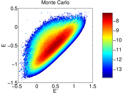
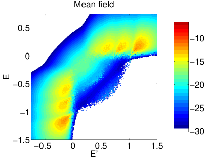
We observe clearly what we discussed in Sec. II. The modified mean field rates closely follow the Monte Carlo results, while the original mean field rates are smaller for transitions crossing the Fermi level ($E<0$ and $E^{\prime}>0$).

VI Conductance

We also calculated the conductance in all three models. In the Monte Carlo simulations this was done by applying an electric field $E_{f}$ in the $x$-direction. This modifies the energy change to $\Delta\epsilon_{ij}=\epsilon_{j}-\epsilon_{i}-1/r_{ij}-E_{f}\Delta x_{ij}$. The transition rates must then be calculated using this energy change but othervise the simulation is as in the equilibrium case. The current is measured directly as the transferred charge in the direction of the field.

In the mean field calculations we find the Miller-Abrahams resistances Miller and Abrahams (1960) $R_{ij}=T/\gamma_{ij}^{0}$ and construct the resistance network. In this case we do not use periodic boundary conditions in the direction of the field. Rather, we set all sites on the left edge to one potential and all on the right to a different potential. We then solve the Kirchhoff equations for the network to find the current in each resistor.

The temperature dependence of the conductance is shown in Fig. 5 for the three models.

Figure 5: Logarithm of conductivity vs. $T^{-1/2}$ for Monte Carlo and mean field results, as specified in legend. Solid lines show linear fits at low temperatures, while markers are the results obtained from calculations/simulations.

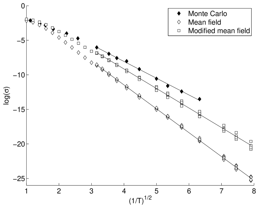
We see that all models follow closely the Efros-Shklovskii law (2), except at high temperatures where the conductance becomes temperature independent. At high temperatures all three models give close to the same conductance. At lower temperatures the mean field approach underestimates the conductance. There are two reasons for this. First, the mean field equations underestimates the number of states close to the bottom of the Coulomb gap. This means that the number of sites which are partially occupied, and active in transport is underestimated. Second, the original mean field transition rates are too small for an important class of transitions as discussed in Sec. V. The modified mean field rates corrects the second problem, and we see that this brings the results into much closer agreement with the Monte Carlo simulations. Assuming the Efros-Shklovskii law to hold, we can extract $T_{0}$ from linear fits to the data. We obtain (in units of $e^{2}/\kappa a$) $T_{0}=5.9\pm 0.4$ (Monte Carlo), $T_{0}=8.0\pm 0.1$ (MLMF) and $T_{0}=12.0\pm 0.05$ (original LMF). It turns out that a self-consistent type of percolation approach based on the ESMF (see Ref. Levin et al., 1987 and references therein) produces good values for $T_{0}$. In particular, for two-dimensional case $T_{0}=6.5\pm 1$.Nguen (1984); Nguyen et al. (2006) Note that the results for $T_{0}$ of the MLMF and ESMF are significantly closer to those of the Monte Carlo calculation than the results of the original LMF. The difference between the the MFLM and the ESMF is that the MFLM takes into account (if only approximately, as discussed in Sec. IV) the smearing of the Coulomb gap at finite temperature. This increases the density of states close to the Fermi level, and we expect that it increases the conductance. This effect should be more pronounced at higher temperatures, and therefore it is natural that $T_{0}$ is larger when this effect is included, and this is indeed what we see. Why the ESMF gives a value closer to the Monte Carlo results is not clear, and it would be instructive to compare the values of the conductance, not only $T_{0}$. In any case, the difference is not very large, and we conclude that the smearing of the Coulomb gap is not of great significance for DC conductance.

VII Summary

We have tested the recently proposed local mean field theory of the Coulomb glass Amir et al. (2008, 2009) and compared it to Monte Carlo simulations. We have also proposed a modified expression for the mean field transition rates to take into account correlations at the most basic level that a jump must take place from an empty to an occupied site.

We have found that the LMF equations underestimate the number of sites in the Coulomb gap at finite temperatures. They will also underestimate the number of sites with intermediate occupation probability, resulting in occupation numbers that are close to either 0 (empty site) or 1 (filled site).

The transition rates of the original mean field equations are strongly underestimated for an important class of transitions, where an electron jumps from below to above the Fermi level, but the distance is short enough so that the self interaction will compensate for the increase in SPE.

The conductance follows closely the ES law in Monte Carlo simulations and both the LMF calculations. However, the LMF gives values of the current smaller than what is seen in the Monte Carlo simulations. The difference is largest when using the original LMF expression for the rates. The MLMF rates come much closer to the simulation results, indicating that a major part of the correlations in the system can be understood in the simple pair approximation used. More complicated correlations, involving three or more sites certainly exist, but seem to be of less importance. The MLMF results are also close to what was found using the ESMF, indicating that the smearing of the Coulomb gap is not important in determining DC conductance. This is not surprising since at very low temperatures, $T\ll T_{0}$, the typical energy band contributing to conductance, $\sim(TT_{0})^{1/2}$, is much larger than temperature.

This work is part of the master project of one of the authors (EB) and more details can be found in his thesis.Bardalen (2011)