Combinatorial Morse flows are hard to find

Abstract.

We investigate the probability of detecting combinatorial Morse flows on a simplicial complex via a random search. We prove that it is really small, in a quantifiable way.

1. Introduction

Let $X$ be a compact space equipped with a triangulation $\mathcal{F}$. Here $\mathcal{F}$ stands for the collection of all the closed faces of the triagulation. The collection $\mathcal{F}$ is a poset with the order relation given by inclusion. For any function $f:\mathcal{F}\rightarrow{\mathbb{R}}$, and any face ${\sigma}\in\mathcal{F}$ we define

$$A_{>{\sigma}}(f):=\bigl{\{}\tau\in\mathcal{F};\;\;\dim\tau=\dim{\sigma}+1,\;\;f(\tau)\leq f({\sigma})\,\bigr{\}},$$

$$A_{<{\sigma}}(f):=\bigl{\{}\tau\in\mathcal{F};\;\;\dim\tau=\dim{\sigma}-1,\;\;f(\tau)\geq f({\sigma})\,\bigr{\}},$$

$$A_{\sigma}(f):=A_{>{\sigma}}(f)\cup A_{<{\sigma}}(f).$$

Following R. Forman [4], we define a combinatorial Morse function to be a function $f:\mathcal{F}\to{\mathbb{R}}$ such that

$$|A_{\sigma}(f)|\leq 1,\;\;\forall{\sigma}\in\mathcal{F}.$$

A face ${\sigma}$ such that $|A_{\sigma}(f)|=0$ is called a critical face of the combinatorial Morse function. Let us observe that the function

$$\mathcal{F}\ni{\sigma}\mapsto\dim{\sigma}$$

is a combinatorial Morse function. All the faces are critical for this function.

Recall that the Hasse diagram of the triangulation $\mathcal{F}$ is the directed graph $\mathcal{H}(\mathcal{F})$ whose vertex set is $\mathcal{F}$, while the set of edges $E(\mathcal{F})$ is defined as follows: we have an edge going from ${\sigma}\in\mathcal{F}$ to $\tau\in\mathcal{F}$ if and only if

$$\dim{\sigma}-\dim\tau=1\;\;\mbox{and}\;\;{\sigma}\supset\tau.$$

To any function ${\boldsymbol{\omega}}:E(\mathcal{F})\to\{\pm 1\}$, and any face ${\sigma}\in\mathcal{F}$ we associate the sets

$$A_{>{\sigma}}({\boldsymbol{\omega}}):=\bigl{\{}\tau\in\mathcal{F};\;\;\overrightarrow{\tau{\sigma}}\in E(\mathcal{F}),\;\;{\boldsymbol{\omega}}(\overrightarrow{\tau{\sigma}})=-1\,\bigr{\}},$$

$$A_{<{\sigma}}({\boldsymbol{\omega}}):=\bigl{\{}\tau\in\mathcal{F};\;\;\overrightarrow{{\sigma}\tau}\in E(\mathcal{F}),\;\;{\boldsymbol{\omega}}(\overrightarrow{{\sigma}\tau})=-1\,\bigr{\}},$$

$$A_{\sigma}({\boldsymbol{\omega}})=A_{>{\sigma}}({\boldsymbol{\omega}})\cup A_{<{\sigma}}({\boldsymbol{\omega}}).$$

We will refer to a function ${\boldsymbol{\omega}}:E(\mathcal{F},{\boldsymbol{\omega}})\to\{\pm 1\}$ as an orientation prescription of $\mathcal{F}$, and we will denote by $\mathcal{O}_{\mathcal{F}}$ the collection of all orientation prescriptions of $\mathcal{F}$.

Any orientation prescription ${\boldsymbol{\omega}}$ defines a new directed graph $\mathcal{H}(\mathcal{F},{\boldsymbol{\omega}})$ whose vertex set is $\mathcal{F}$ and its set of edges $E(\mathcal{F},{\boldsymbol{\omega}})$ is defined as follows.

• The undirected graphs $\mathcal{H}(\mathcal{F})_{0}$ and $\mathcal{H}(\mathcal{F},{\boldsymbol{\omega}})_{0}$ have the same sets of edges.

• If ${\boldsymbol{e}}$ is a directed edge of $\mathcal{H}(\mathcal{F})$, and ${\boldsymbol{\omega}}({\boldsymbol{e}})=1$, then ${\boldsymbol{e}}$ is an edge of $\mathcal{H}(\mathcal{F},{\boldsymbol{\omega}})$. Otherwise, switch the orientation of ${\boldsymbol{e}}$.

Any combinatorial Morse function $f:\mathcal{F}\rightarrow{\mathbb{R}}$ defines an orientation prescription ${\boldsymbol{\omega}}_{f}:E(\mathcal{F})\rightarrow{\mathbb{R}}$ as follows. If $\overrightarrow{{\sigma}\tau}$ is a directed edge of $\mathcal{H}(\mathcal{F})$ then

$${\boldsymbol{\omega}}_{f}\bigl{(}\,\overrightarrow{{\sigma}\tau}\,\bigr{)}=-1{\Longleftrightarrow}\tau\in A_{<{\sigma}}(f)$$

$${\Longleftrightarrow}\dim{\sigma}-\dim\tau=1,\;\;\tau\subset{\sigma},\;\;f(\tau)\geq f({\sigma}).$$

Observe that the Morse condition implies that the directed graph $\mathcal{H}(\mathcal{F},{\boldsymbol{\omega}}_{f})$ has no (directed) cycles. Moreover

$$A_{>{\sigma}}({\boldsymbol{\omega}}_{f})=A_{>{\sigma}}(f),\;\;A_{<{\sigma}}({\boldsymbol{\omega}}_{f})=A_{<{\sigma}}(f).$$

We define a combinatorial flow on $\mathcal{F}$ to be an orientation prescription ${\boldsymbol{\omega}}:E(\mathcal{F})\to{\mathbb{R}}$ such that

$$|A_{\sigma}({\boldsymbol{\omega}})|=1,\;\;\forall{\sigma}\in\mathcal{F}.$$

If ${\boldsymbol{\omega}}$ defines a combinatorial flow, then the set of directed edges ${\boldsymbol{e}}\in E(F)$ such that ${\boldsymbol{\omega}}({\boldsymbol{e}})=-1$ define a matching (in the sense of [6, Def. 11.1]) of the poset of faces $\mathcal{F}$.

Observe that the orientation prescription determined by a combinatorial Morse function is a combinatorial flow. We will refer to such flows as combinatorial Morse flows. Conversely, [6, Thm. 11.2], a combinatorial flow is Morse if and only if it is acyclic, i.e., the directed graph $\mathcal{H}(\mathcal{F},{\boldsymbol{\omega}})$ is acyclic. In topological applications the combinatorial flow determined by a combinatorial Morse function plays the key role. In fact, once we have an acyclic combinatorial flow one can very easily produce a Morse function generating it. A natural question then arises.

How can one produce acyclic combinatorial flows?

The present paper grew out of our attempts to answer this question. Here is a simple strategy. Suppose that by some means we have detected an orientation prescription ${\boldsymbol{\omega}}$ that generates a combinatorial flow. We denote by $\operatorname{sign}{\boldsymbol{\omega}}$ the number of edges ${\boldsymbol{e}}\in E(\mathcal{F})$ such that ${\boldsymbol{\omega}}({\boldsymbol{e}})=-1$. We will deform ${\boldsymbol{\omega}}$ to an acyclic flow using the following procedure.

Step 1. If $\mathcal{H}(\mathcal{F},{\boldsymbol{\omega}})$ is acyclic, then STOP.

Step 2. If $\mathcal{H}(\mathcal{F},{\boldsymbol{\omega}})$ contain cycles, choose one. Then at least one of the edges along this cycle belongs to the set $\{{\boldsymbol{\omega}}=-1\}$. Chose one such edge ${\boldsymbol{e}}$ and define a new orientation prescription ${\boldsymbol{\omega}}^{\prime}$ which is equal to ${\boldsymbol{\omega}}$ on any edge other that ${\boldsymbol{e}}$, whereas ${\boldsymbol{\omega}}^{\prime}({\boldsymbol{e}})=-{\boldsymbol{\omega}}({\boldsymbol{e}})=1$. Note that $\operatorname{sign}{\boldsymbol{\omega}}^{\prime}=\operatorname{sign}{\boldsymbol{\omega}}-1$. GOTO Step 1.

The above procedure reduces the problem to producing combinatorial flows. We have attempted a probabilistic approach. Switch randomly and independently the orientations of the edges in $E(F)$. How likely is it that the resulting orientation prescription defines a combinatorial flow?

More precisely, we equip the set of orientation prescriptions $\mathcal{O}_{\mathcal{F}}$ with the uniform probability measure, and we denote by $\boldsymbol{P}(\mathcal{F})$ the probability that a random orientation prescription is a combinatorial flow. We are interested in estimating this probability when $\mathcal{F}$ is large.

Note that if $\mathcal{F}^{\prime}$ denotes a subcomplex of $\mathcal{F}$, then $\boldsymbol{P}(\mathcal{F})\leq\boldsymbol{P}(\mathcal{F}^{\prime})$. In particular, if $\mathcal{F}_{1}$ denotes the $1$-skeleton of the triangulation, then $\boldsymbol{P}(\mathcal{F})\leq\boldsymbol{P}(\mathcal{F}_{1})$. For this reason we will concentrate excusively on $1$-dimensional complexes, i.e., graphs.

Consider a graph $\Gamma$ with vertex set $V(\Gamma)$ and edge set $E(\Gamma)$. If $E(\Gamma)=\emptyset$, i.e., $\Gamma$ consists of isolated points, then trivially $\boldsymbol{P}(\Gamma)=1$.

Suppose that $E(\Gamma)\neq\emptyset$. If we regard $\Gamma$ as a $1$-dimensional simplicial complex, then its barycentric subdivision is the graph $\Gamma^{\prime}$ obtained by marking the midpoints of the edges of $\Gamma$. The vertices of $\mathcal{H}(\Gamma)$, the Hasse diagram of $\Gamma$, consist of the vertices ${\boldsymbol{v}}$ of $\Gamma$ together with the midpoints $b_{\boldsymbol{e}}$ of the edges ${\boldsymbol{e}}$ of $\Gamma$. To each edge ${\boldsymbol{e}}$ of $\Gamma$ one associates a pair of directed edges of the Hasse diagram, running from the midpoint $b_{\boldsymbol{e}}$ of that edge towards the endpoints of that edge.

Define the incidence relation ${\mathcal{I}}_{\Gamma}\subset V(\Gamma)\times E(\Gamma)$ where $({\boldsymbol{v}},{\boldsymbol{e}})\in{\mathcal{I}}_{\Gamma}$ if and only if the vertex ${\boldsymbol{v}}$ is an endpoint of the edge ${\boldsymbol{e}}$. Note that ${\mathcal{I}}_{\Gamma}$ can be identified with the set of edges of the barycentric subdivision $\Gamma^{\prime}$. An orientation prescription is then a function ${\boldsymbol{\omega}}:{\mathcal{I}}_{\Gamma}\rightarrow\{\pm 1\}$. The edge $({\boldsymbol{v}},b_{\boldsymbol{e}})$ of $\Gamma^{\prime}$ is given the orientation $b_{\boldsymbol{e}}\to{\boldsymbol{v}}$ in the digraph $\mathcal{H}(\Gamma,{\boldsymbol{\omega}})$ if and only if ${\boldsymbol{\omega}}({\boldsymbol{v}},{\boldsymbol{e}})=1$.

We denote by $\mathcal{O}_{\Gamma}$ the set of orientation prescriptions on $\Gamma$ and by $\Phi_{\Gamma}\subset\mathcal{O}_{\Gamma}$ the set of combinatorial flows. Thus, an orientation prescription ${\boldsymbol{\omega}}$ defines a combinatorial flow if the digraph $\mathcal{H}(\Gamma,{\boldsymbol{\omega}})$ has the property at each ${\boldsymbol{v}}\in V(\Gamma)$ there exists at most one outgoing edge, and at each barycenter $b_{\boldsymbol{e}}$ there exists at most one incoming edge.

In Figure 1 we have described orientation prescriptions on the simplical complex defined by the boundary of a square. The orientation prescription in the left-hand side defines an acyclic combinatorial flow, and the numbers assigned to the various vertices describe a combinatorial Morse function defining this flow. The orientation prescription in the right- hand side does not determine a combinatorial flow.

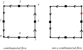
Figure 1. The vertices of $\Gamma$ are marked with $\bullet$’s and the barycenters of the edges are marked with $\blacksquare$’s.

We denote by $\boldsymbol{P}(\Gamma)$ the probability that an orientation prescription is a combinatorial flow, i.e.,

$$\boldsymbol{P}(\Gamma)=\frac{|\Phi_{\Gamma}|}{|\mathcal{O}_{\Gamma}|}=\frac{|\Phi_{\Gamma}|}{4^{N_{\Gamma}}},\;\;N_{\Gamma}=|E(\Gamma)|.$$

The above definition implies trivially that

$$\boldsymbol{P}(\Gamma)\geq\frac{1}{4^{N_{\Gamma}}}.$$ (1.1)

Consider the graph $\boldsymbol{L}_{1}$ consisting of two vertices $v_{0},v_{1}$ connected by an edge. It is easy to see that (see Figure 2)

$$\boldsymbol{P}(\boldsymbol{L}_{1})=\frac{3}{4}.$$

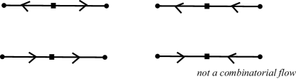
Figure 2. There are four orientation prescriptions on $\boldsymbol{L}_{1}$ and only one of them is not a combinatorial flow

If ${\boldsymbol{\omega}}$ is an orientation prescription on a graph $\Gamma$, then it defines a combinatorial flow only if its restriction to each of the edges (viewed as copies of $\boldsymbol{L}_{1}$) are combinatorial flows. We deduce

$$\boldsymbol{P}(\Gamma)\leq\left(\frac{3}{4}\right)^{N_{\Gamma}}$$ (1.2)

Note that the above upper bound is optimal: we have equality when $\Gamma$ consists of disjoint edges. Already this shows that the above probabilistic approach has very small chances of success. However, we wish to say something more.

Motivated by the estimates (1.1) and (1.2) we introduce a new invariant

$$\boldsymbol{h}(\Gamma):=\begin{cases}\frac{\log\boldsymbol{P}(\Gamma)}{N_{\Gamma}},&E(\Gamma)\neq\emptyset\\ 0,&E(\Gamma)=\emptyset.\end{cases}$$

The inequalities (1.1) and (1.2) can be rewritten as

$$E(\Gamma)\neq\emptyset\Rightarrow\log\left(\frac{1}{4}\right)\leq\boldsymbol{h}(\Gamma)\leq\log\left(\frac{3}{4}\right).$$ (1.3)

In this paper we investigate the invariant $\boldsymbol{h}(\Gamma)$ for various classes of graphs and study its behavior as $\Gamma$ becomes very large. In particular, we prove that the inequalities (1.3) are optimal.

The above lower bound is also an asymptotically optimal bound. More precisely the arguments in this paper show that

$$\log\left(\frac{1}{4}\right)=\liminf_{\begin{subarray}{c}N_{\Gamma}\to\infty,\\ b_{0}(\Gamma)=1\end{subarray}}\boldsymbol{h}(\Gamma),$$

where $b_{0}(\Gamma)$ denotes the number of connected components of $\Gamma$. The same cannot be said about the upper bound. in is not hard to see that

$$\limsup_{\begin{subarray}{c}N_{\Gamma}\to\infty,\\ b_{0}(\Gamma)=1\end{subarray}}\boldsymbol{h}(\Gamma)<\log\left(\frac{3}{4}\right).$$

Moreover, the results in Section 3 show that

$$\limsup_{\begin{subarray}{c}N_{\Gamma}\to\infty,\\ b_{0}(\Gamma)=1\end{subarray}}\boldsymbol{h}(\Gamma)\geq\log\left(\frac{3+\sqrt{5}}{8}\right).$$

We are inclined to believe that in fact we have equality above.

The paper is structured as follows. In Section 2 we describe several general techniques for computing $\boldsymbol{P}(\Gamma)$. In Section 3 we use these general techniques to compute $\boldsymbol{P}(\Gamma)$ for several classes of graphs $\Gamma$. In Section 4 we describe several general properties of $\boldsymbol{h}(\Gamma)$ and formulate several problems that we believe are interesting.

2. General facts concerning combinatorial flows on graphs

Consider a graph $\Gamma$ with vertex set $V(\Gamma)$ and edge set $E(\Gamma)\neq\emptyset$. To ${\boldsymbol{\omega}}\in\mathcal{O}_{\Gamma}$ we associate an anomaly function $A_{\boldsymbol{\omega}}:V(\Gamma)\rightarrow{\mathbb{Z}}_{\geq 0}$, where for any ${\boldsymbol{v}}\in V(\Gamma)$ we denote by $A_{\boldsymbol{\omega}}({\boldsymbol{v}})$ the number of edges of the digraph $\mathcal{H}(\Gamma,{\boldsymbol{\omega}})$ that exit the vertex ${\boldsymbol{v}}$. For any subset $S\subset V(\Gamma)$ and any function $f:S\rightarrow{\mathbb{Z}}_{\geq 0}$ we denote by $\boldsymbol{P}_{S}(\Gamma|\,f\,)$ the conditional probability that the orientation prescription ${\boldsymbol{\omega}}\in\mathcal{O}_{\Gamma}$ is a combinatorial flow given that $A_{\boldsymbol{\omega}}|_{S}=f$. Note that $\boldsymbol{P}_{S}(\Gamma|f)=0$ if $\max f>1$ and

$$\boldsymbol{P}(\Gamma)=\sum_{f:V(\Gamma)\to\{0,1\}}\boldsymbol{P}_{V(\Gamma)}\bigl{(}\,\Gamma\;\bigl{|}\;f\,\bigr{)}.$$ (2.1)

The above conditional probabilities satisfy two very simple rules, the product rule and the quotient rule.

The product rule explains what happens with the various probabilities when we take the disjoint union of two graphs. More precisely, suppose we are given disjoint graphs $\Gamma_{i}$, subsets $S_{i}\subset V(\Gamma_{i})$ and functions $f_{i}:S_{i}\to{\mathbb{Z}}_{\geq 0}$, $i=1,2$. Then

$$\boldsymbol{P}_{S_{1}\sqcup S_{2}}\bigl{(}\Gamma_{1}\sqcup\Gamma_{2}\,\bigl{|}\;f_{1}\sqcup f_{2}\,\bigl{)}=\boldsymbol{P}_{S_{1}}\bigl{(}\,\Gamma_{1}\;\bigl{|}\;f_{1}\,\bigr{)}\cdot\boldsymbol{P}_{S_{2}}\bigl{(}\,\Gamma_{2}\;\bigl{|}\;f_{2}\,\bigr{)},$$ (2.2)

The product rule explains what happens with the various probabilities when we identify several vertices in a graph, thus obtaining a new graph with fewer vertices but the same number of edges.

Suppose that we are given a graph $\Gamma$ and an equivalence relation ”$\sim$” on $V(\Gamma)$. Denote by $\bar{\Gamma}$ the graph obtained from $\Gamma$ by identifying vertices via the equivalence relation $\sim$. Denote by $\pi$ the natural projection

$$\pi:V(\Gamma)\to V(\Gamma)/\sim=V(\bar{\Gamma}).$$

Fix a subset $\bar{S}\subset V(\bar{\Gamma})$ and a function $\bar{f}:\bar{S}\to{\mathbb{Z}}_{\geq 0}$. We denote by $S$ the preimage $S:=\pi^{-1}(S)$. To any function $g:S\to{\mathbb{R}}$ we associate a function

$$\pi_{*}(g):\bar{S}\to{\mathbb{R}},$$

obtained by integrating $g$ along the fibers of $\pi$, i.e.

$$\pi_{*}(g)(\bar{s}):=\sum_{s\in\pi^{-1}(\bar{s})}g(s),\;\;\forall\bar{s}\in\bar{S}.$$

The quotient rule the states

$$\boldsymbol{P}_{\bar{S}}\bigl{(}\,\bar{\Gamma}\;\bigl{|}\;\bar{f}\;\bigl{)}=\sum_{\pi_{*}(f)=f}\boldsymbol{P}_{S}\bigl{(}\,\Gamma\;\bigl{|}\;f\,\bigr{)},\;\;\forall\bar{f}:\bar{S}\rightarrow\{0,1\}.$$ (2.3)

In particular

$$\boldsymbol{P}(\bar{\Gamma})=\sum_{\pi_{*}(f)\leq 1}\boldsymbol{P}_{V(\Gamma)}\bigl{(}\,\Gamma\;\bigl{|}\;f\,\bigr{)}.$$ (2.4)

Example 2.1.

Consider the graph $\boldsymbol{L}_{1}$ consisting of two vertices $v_{0},v_{1}$ connected by an edge. A function ${\epsilon}:V(\boldsymbol{L}_{1})\to\{0,1\}$ is determined by two numbers ${\epsilon}_{i}={\epsilon}(v_{i})$. We set

$$p_{1}({\epsilon}_{0},{\epsilon}_{1}):=\boldsymbol{P}_{V(\boldsymbol{L}_{1})}(\boldsymbol{L}_{1}\,|\;{\epsilon}).$$

An inspection of Figure 2 shows that

$$p_{1}(0,1)=p_{1}(1,0)=p_{1}(0,0)=\frac{1}{4},\;\;p_{1}(1,1)=0.$$

$\hbox to0.0pt{$\sqcap$\hss}\sqcup$

Note that every graph with $n$ edges is a quotient of the graph consisting of $n$ disjoint copies of $\boldsymbol{L}_{1}$, we can use (2.1), (2.2) and (2.3) a produce a formula formula for $\boldsymbol{P}(\Gamma)$.

Given a graph $\Gamma$ we introduce formal variables $\vec{z}:=(z_{v})_{v\in V(\Gamma)}$. To an edge ${\boldsymbol{e}}$ of $\Gamma$ with endpoints $v_{0},v_{1}$ we associate the polynomial

$$Q_{\boldsymbol{e}}(\vec{z}):=\sum_{{\epsilon}_{0},{\epsilon}_{1}\leq 1}p_{1}({\epsilon}_{0},{\epsilon}_{1})z_{v_{0}}^{{\epsilon}_{0}}z_{v_{1}}^{{\epsilon}_{1}}=\frac{1}{4}(1+z_{0}+z_{1})=\frac{1}{4}\bigl{(}\,(1+z_{0})(1+z_{1})-z_{0}z_{1}\,\bigr{)}.$$

We define

$$Q_{\Gamma}(\vec{z}):=\prod_{{\boldsymbol{e}}\in E(\Gamma)}Q_{\boldsymbol{e}}.$$

Then the quotient rule (2.4) implies

$$\boldsymbol{P}(\Gamma)=\sum_{S\subset V(\Gamma)}\partial_{S}Q_{\Gamma}|_{\vec{z}=0},$$ (2.5)

where for any subset $S=\{v_{1},\dotsc,v_{k}\}\subset V(\Gamma)$ we define

$$\partial_{S}:=\frac{\partial^{k}}{\partial z_{v_{1}}\dotsc\partial z_{v_{k}}}.$$

Observe that the term $\partial_{S}Q_{\Gamma}|_{\vec{z}=0}$ involves only the subgraph $\widetilde{\Gamma}_{S}$ of $\Gamma$ formed by the edges incident to the vertices in $S$.

It is convenient to regard $Q_{\Gamma}$ as a (polynomial) function on the vector space ${\mathbb{C}}^{V(\Gamma)}$ with coordinates $(z_{v})_{v\in V(\Gamma)}$. If $\sim$ is an equivalence relation on $V(\Gamma)$ and $\bar{\Gamma}$ denotes the graph $\Gamma/\sim$, then we can identify ${\mathbb{C}}^{V(\bar{\Gamma})}$ with the subspace of ${\mathbb{C}}^{V(\Gamma)}$ given by the linear equations

$$z_{u}=z_{v}{\Longleftrightarrow}u\sim v.$$

Moreover

$$Q_{\bar{\Gamma}}=Q_{\Gamma}|_{{\mathbb{C}}^{V(\bar{\Gamma})}}.$$

For any multi-index $\alpha\in{\mathbb{Z}}_{\geq 0}^{V(\Gamma)}$ we set

$$\vec{z}^{\alpha}=\prod_{v}z_{v}^{\alpha_{v}}.$$

For any polynomial

$$P=\sum_{\alpha}p_{\alpha}\vec{z}^{\alpha}\in{\mathbb{C}}[(z_{v})_{v\in V(\Gamma)}]$$

we define its truncation

$$\boldsymbol{T}[P]=\sum_{\alpha_{v}\leq 1}p_{\alpha}\vec{z}^{\alpha}.$$

Any subset $S\subset V(\Gamma)$ defines a multi-index $\alpha=\alpha_{S}\in{\mathbb{Z}}_{\geq 0}^{V(\Gamma)}$, $\alpha_{v}=1$ if $v\in S$, $\alpha_{v}=0$ if $v\not\in S$. We write

$$\vec{z}^{S}:=\vec{z}^{\alpha_{S}},\;\;p_{S}:=p_{\alpha_{S}},$$

so that the truncated polynomial has the form

$$\boldsymbol{T}[P]=\sum_{S\subset V(\Gamma)}p_{S}\vec{z}^{S}.$$

The equality (2.5) can be rewritten as

$$\boldsymbol{P}(\Gamma)=\boldsymbol{T}[Q_{\Gamma}](1).$$ (2.6)

3. Combinatorial flows on various classes of graphs

In the sequel we will denote by $I_{n}$ the set $\{1,\dotsc,n\}$.

Theorem 3.1.

Denote by $\boldsymbol{S}_{n}$ the star shaped graph consisting of $n+1$ vertices $v_{0},v_{1},\dotsc,v_{n}$ and $n$ edges $[v_{0},v_{1}],\dotsc,[v_{0},v_{n}]$. Then

$$\boldsymbol{T}[Q_{\boldsymbol{S}_{n}}]=\frac{1}{4^{n}}\sum_{S\subset I_{n}}\vec{z}^{S}+\frac{1}{4^{n}}\sum_{S\subset I_{n}}(n-|S|)z_{0}\vec{z}^{S},$$ (3.1)

$$\boldsymbol{P}(\boldsymbol{S}_{n})=\frac{n+2}{2^{n+1}},$$ (3.2)

and

$$\boldsymbol{h}(\boldsymbol{S}_{n})\sim\log\left(\frac{1}{2}\right)\;\;\mbox{as $n\to\infty$}.$$ (3.3)

Proof.

We have

$$4^{n}Q_{\boldsymbol{S}_{n}}=\sum_{S\subset I_{n}}\prod_{i\in S}(z_{0}+z_{i})$$

so that

$$4^{n}\boldsymbol{T}[Q_{\boldsymbol{S}_{n}}]=\sum_{S\subset I_{n}}\boldsymbol{T}\left[\prod_{i\in S}(z_{0}+z_{i})\right]$$

$$\sum_{S\subset I_{n}}\left(\prod_{i\in S}z_{i}+z_{0}\sum_{j\in S}\prod_{i\in S\setminus j}z_{i}\right)=\sum_{S\subset I_{n}}\vec{z}^{S}+z_{0}\sum_{S\subset I_{n}}(n-|S|)\vec{z}^{S}.$$

Hence

$$\boldsymbol{P}(\boldsymbol{S}_{n})=\frac{1}{4^{n}}\sum_{k=0}^{n}(n-k+1)\binom{n}{k}=\frac{1}{2^{n}}+\frac{1}{4^{n}}\sum_{k=0}^{n}(n-k)\binom{n}{n-k}$$

$$=\frac{1}{2^{n}}+\frac{1}{4^{n}}\underbrace{\sum_{j=1}^{n}j\binom{n}{j}}_{=n2^{n-1}}=\frac{n+2}{2^{n+1}}.$$

The estimate (3.3) is now obvious. $\hbox to0.0pt{$\sqcap$\hss}\sqcup$

Theorem 3.2.

Denote by $\boldsymbol{L}_{n}$ the graph with $n+1$-vertices $v_{0},v_{1}\dotsc,v_{n}$ and $n$ edges

$$[v_{0},v_{1}],[v_{1},v_{2}],\dotsc,[v_{n-1},v_{n}].$$

We set $p_{n}=p(\boldsymbol{L}_{n})$ and

$$p_{n}:=p(\boldsymbol{L}_{n}),\;\;p(z):=\sum_{n\geq 1}p_{n}z^{n}.$$

Then

$$\sum_{n\geq 1}p_{n}z^{n}=\frac{12z-z^{2}}{(z^{2}-12z+16)}=\frac{16}{(z^{2}-12z+16)}-1.$$ (3.4)

In particular

$$\boldsymbol{h}(\boldsymbol{L}_{n})\sim\log r\;\;\mbox{as $n\to\infty$},$$ (3.5)

where

$$r=\frac{3+\sqrt{5}}{8}\approx 0.654<\frac{3}{4}.$$ (3.6)

Proof.

For ${\epsilon},{\epsilon}^{\prime}\in\{0,1\}$ we set

$$p_{n}({\epsilon})=\boldsymbol{P}\bigl{(}{\boldsymbol{\omega}}\in\Phi_{\Gamma_{n}}\;\bigl{|}\;A_{\boldsymbol{\omega}}(v_{0})={\epsilon}\,\bigr{)}=\boldsymbol{P}\bigl{(}{\boldsymbol{\omega}}\in\Phi_{\Gamma_{n}}\;\bigl{|}\;A_{\boldsymbol{\omega}}(v_{n})={\epsilon}\,\bigr{)},$$

$$p_{n}({\epsilon},{\epsilon}^{\prime})=\boldsymbol{P}\bigl{(}{\boldsymbol{\omega}}\in\Phi_{\Gamma_{n}}\;\bigl{|}\;A_{\boldsymbol{\omega}}(v_{0})={\epsilon},A_{\boldsymbol{\omega}}(v_{n})={\epsilon}^{\prime}\,\bigr{)},$$

$$\vec{p_{n}}:=\left[\begin{array}[]{c}p_{n}(0)\\ p_{n}(1)\end{array}\right],\;\;\vec{p_{n}}({\epsilon}):=\left[\begin{array}[]{c}p_{n}(0,{\epsilon})\\ p_{n}(1.{\epsilon})\end{array}\right].$$

Hence $p_{n}=p_{n}(0)+p_{n}(1)$. Note that

$$p_{1}(0)=p_{1}(0,0)+p_{1}(0,1)=\frac{1}{2},\;\;p_{1}(1)=p_{1}(1,0)+p_{1}(1,1)=\frac{1}{4}.$$

The equality (2.2) implies

$$p_{n}(0)=\sum_{{\epsilon}+{\epsilon}^{\prime}\leq 1}p_{1}(0,{\epsilon})p_{n-1}({\epsilon}^{\prime})=\frac{1}{4}\left(\,2p_{n-1}(0)+p_{n-1}(1)\,\right),$$

$$p_{n}(1)=\sum_{{\epsilon}+{\epsilon}^{\prime}\leq 1}p_{1}(1,{\epsilon})p_{n-1}({\epsilon}^{\prime})=\frac{1}{4}\left(\,p_{n-1}(0)+p_{n-1}(1)\,\right).$$

We can rewrite the above equalities in the compact form

$$\vec{p}_{n}=A\vec{p}_{n-1},\;\;A:=\frac{1}{4}\left[\begin{array}[]{cc}2&1\\ 1&1\end{array}\right].$$

We deduce

$$\vec{p}_{n}=A^{n-1}\vec{p}_{1}.$$ (3.7)

We conclude similarly that

$$\vec{p}_{n}({\epsilon})=A^{n-1}\vec{p}_{1}({\epsilon}).$$ (3.8)

The characteristic polynomial of $A$ is

$$\lambda^{2}-\frac{3}{4}\lambda+\frac{1}{16}=0,$$

and its eigenvalues are

$$\lambda_{\pm}=\frac{3\pm\sqrt{5}}{8}.$$

Each of the sequences $p_{n}({\epsilon})$ is a solution of the second order linear recurrence relation

$$x_{n+2}-\frac{3}{4}x_{n+1}+\frac{1}{16}x_{n}=0$$ (3.9)

We deduce that $p_{n}$ also satisfies the above linear recurrence relation so that

$$p(z)=\frac{C^{\prime}z^{2}+B^{\prime}z}{\frac{1}{16}z^{2}-\frac{3}{4}z+1}=\frac{Cz^{2}+Bz}{z^{2}-12z+16},$$

where $C=16C^{\prime}$, $B=16B^{\prime}$ are real constants. Note that

$$\vec{p}_{2}=A\vec{p}_{1}=\frac{1}{16}\left[\begin{array}[]{cc}2&1\\ 1&1\end{array}\right]\cdot\left[\begin{array}[]{c}2\\ 1\end{array}\right]=\left[\begin{array}[]{c}\frac{5}{16}\\ \\ \frac{3}{16}\end{array}\right].$$

Hence $p_{2}=\frac{8}{16}$. Now observe that

$$\frac{1}{z^{2}-12z+16}={\frac{1}{16}}+{\frac{3}{64}}z+O\left({z}^{2}\right).$$

Hence

$$p(z)=\frac{B}{16}z+\left(\frac{3B}{64}+\frac{C}{16}\right)z^{2}+O\left({z}^{3}\right).$$

We deduce that $B=12$, $C=-1$. The estimate (3.5) follows from the above discussion. $\hbox to0.0pt{$\sqcap$\hss}\sqcup$

Remark 3.3.

(a) Using MAPLE we can easily determine the first few values of $p_{n}$. We have

$$p(z)={\frac{3}{4}}z+{\frac{1}{2}}{z}^{2}+{\frac{21}{64}}{z}^{3}+{\frac{55}{256}}{z}^{4}+{\frac{9}{64}}{z}^{5}+{\frac{377}{4096}}{z}^{6}+{\frac{987}{16384}}{z}^{7}+{\frac{323}{8192}}{z}^{8}+O\left({z}^{9}\right).$$

Ultimately, the recurrence (3.9) is the fastest way to compute $p_{n}$ for any $n$.

(b) Note that $\boldsymbol{S}_{2}=\boldsymbol{L}_{2}$. In this case the equality (3.2) is in perfect agreement with the equality $\boldsymbol{P}(\boldsymbol{L}_{2})=\frac{1}{2}$. $\hbox to0.0pt{$\sqcap$\hss}\sqcup$

Example 3.4 (Octopi and dandelions).

(a) We define an octopus of type $(n_{1},\dotsc,n_{k})$, $k\geq 3$, to be the graph $\boldsymbol{O}(n_{1},\dotsc,n_{k})$ obtained by gluing the linear graphs $\boldsymbol{L}_{n_{1}},\dotsc,\boldsymbol{L}_{n_{k}}$ at a common endpoint. The quotient rule implies that

$$\begin{split}\boldsymbol{P}\bigl{(}\,\boldsymbol{O}(n_{1},\dotsc,n_{k})\,\bigr{)}=\prod_{j=1}^{n}p_{n_{j}}(0)+\sum_{j=1}^{n}p_{n_{1}}(0)\cdots p_{n_{j-1}}(0)p_{n_{j}}(1)p_{n_{j+1}}(0)\cdots p_{n_{k}}(0)\\ =\prod_{j=1}^{n}p_{n_{j}}(0)\left(\,1+\sum_{j=1}^{k}\frac{p_{n_{j}}(1)}{p_{n_{j}}(0)}\,\right).\end{split}$$ (3.10)

We write

$$\boldsymbol{O}_{k\times n}:=\boldsymbol{O}_{(}\underbrace{n_{1},\dotsc,n_{k}}_{k}).$$

We deduce

$$\boldsymbol{P}\bigl{(}\,\boldsymbol{O}_{k\times n}\,\bigr{)}=p_{n}(0)^{k}\left(1+k\frac{p_{n}(1)}{p_{n}(0)}\right),\;\;\boldsymbol{h}\bigl{(}\boldsymbol{O}_{k\times n}\,\bigr{)}=\frac{\log p_{n}(0)}{n}+\frac{\log\left(1+k\frac{p_{n}(1)}{p_{n}(0)}\right)}{nk}.$$

(b) The dandelion of type $(n,m)$ is the graph

$$\boldsymbol{D}_{n,m}=\boldsymbol{O}(\,n,\;\underbrace{1,\dotsc,1}_{m}\,).$$

Using (3.10) we deduce

$$\boldsymbol{P}(\boldsymbol{D}_{n,m})=p_{n}(0)\left(\frac{1}{2}\right)^{m}\left(1+\frac{p_{n}(1)}{p_{n}(0)}+\frac{m}{2}\right).$$

$\hbox to0.0pt{$\sqcap$\hss}\sqcup$

Theorem 3.5.

For $n\geq 3$ we denote by $\boldsymbol{C}_{n}$ the cyclic graph with $n$-vertices, i.e., the graph with vertices $v_{1},\dotsc,v_{n}$ and edges

$$[v_{1},v_{2}],\dotsc,[v_{n-1},v_{n}],[v_{n},v_{1}]$$

Then the sequence $\boldsymbol{P}(\boldsymbol{C}_{n})$ satisfies the linear recurrence relation (3.9) with initial conditions

$$\boldsymbol{P}(\boldsymbol{C}_{3})=\frac{9}{32},\;\;\boldsymbol{P}(\boldsymbol{C}_{3})=\frac{47}{256}.$$ (3.11)

In particular

$$\boldsymbol{h}(\boldsymbol{C}_{n})\sim\log r\;\;\mbox{as $n\to\infty$},$$ (3.12)

where $r$ is described by (3.6).

Proof.

The graph $\boldsymbol{C}_{n}$ is obtained from $\boldsymbol{L}_{n}$ by identifying the endpoints $v_{0},v_{n}$ of $\boldsymbol{L}_{n}$. Using (2.3) and the notations in the proof of Theorem 3.6 we deduce that

$$\boldsymbol{P}(\boldsymbol{C}_{n})=\sum_{{\epsilon}+{\epsilon}^{\prime}\leq 1}p_{n}({\epsilon},{\epsilon}^{\prime})=p_{n}(0,0)+p_{n}(0,1)+p_{n}(1,0)=p_{n}(0,0)+2p_{n}(0,1).$$

This shows that $\boldsymbol{P}(\boldsymbol{C}_{n})$ satisfies the recurrence (3.9) since both $p_{n}(0,0)$ and $p_{n}(0,1)$ do. Using (3.8) we deduce

$$\vec{p}_{3}(0)=\frac{1}{4^{2}}A^{2}\vec{p}_{1}(0)=\frac{1}{4^{3}}\left[\begin{array}[]{cc}5&3\\ 3&2\end{array}\right]\cdot\left[\begin{array}[]{c}1\\ 1\end{array}\right]=\left[\begin{array}[]{c}\frac{1}{8}\\ \\ \frac{5}{4^{3}}\end{array}\right]$$

$$\vec{p}_{3}(0)=\frac{1}{4^{4}}\left[\begin{array}[]{cc}13&8\\ 8&5\end{array}\right]\cdot\left[\begin{array}[]{c}1\\ 1\end{array}\right]=\left[\begin{array}[]{c}\frac{21}{4^{4}}\\ \\ \frac{13}{4^{4}}\end{array}\right].$$

This shows that

$$\boldsymbol{P}(\boldsymbol{C}_{3})=\frac{1}{4}+\frac{10}{4^{3}}=\frac{9}{32},\;\;\boldsymbol{P}(\boldsymbol{C}_{4})=\frac{21}{4^{4}}+\frac{26}{4^{4}}=\frac{47}{256}=0.18359375.$$

$\hbox to0.0pt{$\sqcap$\hss}\sqcup$

Theorem 3.6.

Denote by ${\boldsymbol{K}}_{n}$ the complete graph with $n$ vertices. Then

$$\frac{1}{4^{\frac{n(n-1)}{2}}}\left(1+\frac{n}{2}\right)^{n}\leq\boldsymbol{P}({\boldsymbol{K}}^{n})\leq\frac{1}{4^{\frac{n(n-1)}{2}}}(n+1)^{n}.$$ (3.13)

In particular

$$\boldsymbol{h}({\boldsymbol{K}}_{n})\sim\log\left(\frac{1}{4}\right)\;\;\mbox{as $n\to\infty$}.$$ (3.14)

Proof.

We have

$$Q_{{\boldsymbol{K}}_{2}}=\frac{1}{4}\boldsymbol{T}[Q_{{\boldsymbol{K}}_{2}}]=\frac{1}{4}(1+z_{1}+z_{2}),$$

$$\begin{split}\boldsymbol{T}[Q_{{\boldsymbol{K}}_{3}}]=\frac{1}{4^{3}}\boldsymbol{T}\left[\,(1+z_{1}+z_{2})\cdot\boldsymbol{T}\bigl{[}(1+z_{1}+z_{3})(1+z_{2}+z_{3})\,\bigr{]}\,\right]\\ =\frac{1}{4^{3}}\boldsymbol{T}\left[\,(1+z_{1}+z_{2})\cdot(1+z_{1}+z_{2}+2z_{3}+z_{1}z_{2}+z_{2}z_{3}+z_{3}z_{1})\right]\\ =\frac{1}{4^{3}}\bigl{(}\,1+2(z_{1}+z_{2}+z_{3})+3(z_{1}z_{2}+z_{2}z_{3}+z_{3}z_{1})+2z_{1}z_{2}z_{3}\,\bigr{)}.\end{split}$$ (3.15)

In general, we write

$$\boldsymbol{T}[Q_{{\boldsymbol{K}}_{n}}]=\frac{1}{4^{\frac{n(n-1)}{2}}}\sum_{S\subset I_{n}}c_{n}(S)\vec{z}^{S},$$ (3.16)

where we recall that

$$N_{{\boldsymbol{K}}_{n}}=\binom{n}{2}=\frac{n(n-1)}{2}.$$

Observe that

$$c_{n}(S)=c_{n}(S^{\prime})\;\;\mbox{if}\;\;|S|=|S^{\prime}|.$$

We denote by $c_{n}(k)$ the common value of the numbers $c_{n}(S)$, $|S|=k$. We can rewrite (3.16) as

$$\boldsymbol{T}[Q_{{\boldsymbol{K}}_{n}}]=\frac{1}{4^{\frac{n(n-1)}{2}}}\sum_{k=0}^{n}c_{n}(k)\left(\sum_{S\subset I_{n},\;|S|=k}\vec{z}^{S}\right).$$ (3.17)

In particular, we deduce that

$$\boldsymbol{P}({\boldsymbol{K}}_{n})=\frac{1}{4^{\frac{n(n-1)}{2}}}\sum_{k=0}^{n}\binom{n}{k}c_{n}(k).$$ (3.18)

Now think of the graph ${\boldsymbol{K}}_{n}$ as obtained from the graph ${\boldsymbol{K}}_{n}$ as obtained from ${\boldsymbol{K}}_{n}$ by adding a new vertex $v_{0}$ and $n$-new edges $[v_{0},v_{k}]$, $k=1,\dotsc,n$. In other words ${\boldsymbol{K}}_{n+1}$ is a quotient of the graph ${\boldsymbol{K}}_{n}\sqcup\boldsymbol{S}_{n}$. Using the product and quotient rules we deduce that

$$\boldsymbol{T}\bigl{[}\,Q_{{\boldsymbol{K}}_{n+1}}(z_{0},\dotsc,z_{n})\,\bigr{]}=\boldsymbol{T}\bigl{[}\;\boldsymbol{T}[Q_{{\boldsymbol{K}}_{n}}](z_{1},\dotsc,z_{n})\cdot\boldsymbol{T}[Q_{\boldsymbol{S}_{n}}](z_{0},z_{1},\dotsc,z_{n})\;\bigr{]}.$$ (3.19)

For $S\subset I_{n}$, $|S|=k$, we deduce from (3.1), (3.16) and (3.19) that

$$c_{n+1}(k)=c_{n+1}(S)=\sum_{S^{\prime}\sqcup S^{\prime\prime}=S}c_{n}(S^{\prime})=\sum_{j=0}^{k}\binom{k}{j}c_{n}(j).$$ (3.20)

If $I_{n}^{*}=\{0\}\cup I_{n}$, then (3.1), (3.16) and (3.19) imply that

$$c_{n+1}(n+1)=c_{n}(I_{n}^{*})=\sum_{S\sqcup S^{\prime}=I_{n}}(n-|S|)c_{n}(S^{\prime})=\sum_{k=0}^{n}k\binom{n}{k}c_{n}(k).$$ (3.21)

Lemma 3.7.

For any $n\geq 3$ and any $0\leq k\leq n$ we have

$$\left(\frac{n}{2}\right)^{k}\leq c_{n}(k)\leq n^{k}.$$ (3.22)

Proof.

We argue by induction on $n$. For $n=3$ the inequalities follow from (3.15). As for the inductive step, observe that if $k<n+1$, then (3.20) implies that

$$c_{n+1}(k)\leq\ \sum_{j=0}^{k}\binom{k}{j}n^{j}=(n+1)^{k}$$

and

$$c_{n+1}(k)\geq\sum_{j=0}^{k}\binom{k}{j}\left(\frac{n}{2}\right)^{j}=\left(1+\frac{n}{2}\right)^{k}>\left(\frac{n+1}{2}\right)^{k}.$$

Next we deduce from (3.21) and the induction assumption that

$$c_{n+1}(n+1)\leq\sum_{k=0}^{n}k\binom{n}{k}n^{k}\leq(n+1)\sum_{k=0}^{n}\binom{n}{k}n^{k}=(n+1)^{n+1}$$

$$c_{n+1}(n+1)\geq\sum_{k=0}^{n}k\binom{n}{k}\left(\frac{n}{2}\right)^{k}.$$

If we let

$$B_{n}(t):=(1+t)^{n},\;\;D_{n}(t):=tB_{n}^{\prime}(t)=nt(1+t)^{n-1}$$

then we deduce that

$$\sum_{k=0}^{n}k\binom{n}{k}\left(\frac{n}{2}\right)^{k}=D_{n}\bigl{(}n/2\bigr{)}=\frac{n^{2}}{2}\left(1+\frac{n}{2}\right)^{n-1}.$$

It remains to check that

$$\frac{n^{2}}{2}\left(1+\frac{n}{2}\right)^{n-1}\geq\left(\frac{n+1}{2}\right)^{n+1},\;\;\forall n\geq 3.$$ (3.23)

Indeed, observe that (3.23) is equivalent to the inequality

$$\left(\frac{n+2}{n+1}\right)^{n-1}\geq\frac{(n+1)^{2}}{2n^{2}},\;\;\forall n\geq 3,$$

which is holds since the right-hand-side is $\leq 1$, $\forall n\geq 3$. $\hbox to0.0pt{$\sqcap$\hss}\sqcup$

Using (3.18) and (3.23) we deduce that

$$\frac{1}{4^{\frac{n(n-1)}{2}}}\sum_{k=0}^{n}\binom{n}{k}\left(\frac{n}{2}\right)^{k}\leq\boldsymbol{P}({\boldsymbol{K}}_{n})\leq\frac{1}{4^{\frac{n(n-1)}{2}}}\sum_{k=0}^{n}\binom{n}{k}n^{k}.$$

This proves (3.13) and completes the proof of Theorem 3.6.

$\hbox to0.0pt{$\sqcap$\hss}\sqcup$

4. Final comments

We want to extract some qualitative information from the quantitative results proved so far. The invariant $\boldsymbol{h}(\Gamma)$ enjoys a monotonicity. More precisely

$$\boldsymbol{h}(\Gamma)\subset\boldsymbol{h}(\Gamma^{\prime})\;\;\mbox{ if $V(\Gamma)\subset V(\Gamma^{\prime})$ and $E(\Gamma)\supset E(\Gamma^{\prime})$}$$ (4.1)

Indeed, we have

$$\boldsymbol{P}(\Gamma)\leq\boldsymbol{P}(\Gamma^{\prime}),\;\;N_{\Gamma}\geq N_{\Gamma^{\prime}}.$$

Next we observe that

$$\boldsymbol{h}(\Gamma\sqcup\Gamma^{\prime})=\frac{N_{\Gamma}}{N_{\Gamma}+N_{\Gamma^{\prime}}}\boldsymbol{h}(\Gamma)+\frac{N_{\Gamma^{\prime}}}{N_{\Gamma}+N_{\Gamma^{\prime}}}\boldsymbol{h}(\Gamma^{\prime}).$$ (4.2)

If we let $\Gamma$ be a complete graph with a large number of vertices and $\Gamma^{\prime}$ be a disjoint union of $m$ edges, then

$$\boldsymbol{h}(\Gamma)\approx\log(1/4),\;\;\boldsymbol{h}(\Gamma^{\prime})=\log(3/4)$$

and by varying $m$ we obtain from (4.2) the following result.

Corollary 4.1.

The discrete set $\{\boldsymbol{h}(\Gamma)\}$ is dense in the interval $[\log(1/4),\log(3/4)]$. $\hbox to0.0pt{$\sqcap$\hss}\sqcup$

Clearly, if $\Gamma_{0}$ and $\Gamma_{1}$ are isomorphic graphs then $\boldsymbol{h}(\Gamma_{0})=\boldsymbol{h}(\Gamma_{1})$. Coupling this with (4.1) we deduce that for any $x\in(\,\log(1/4),\log(3/4)\,)$ the property

$$\boldsymbol{h}(\Gamma)\leq x$$

is a monotone increasing graph property in the sense of [1, §2.1]. We denote by $p_{n}(x,N)$ the probability conditional probability

$$\boldsymbol{P}_{n}(x,N)=\boldsymbol{P}\bigl{(}\,\boldsymbol{h}(\Gamma)\leq x\;\bigl{|}\;|V(\Gamma)|=n,\;\;|E(\Gamma)|=N\,\bigr{)},$$

where the set of graphs with $n$ vertices and $N$-edges is equipped with the uniform probability measure.

The results of [2, 5] show that the property (4) admits a threshold. This means that there exists a function

$$\boldsymbol{m}_{x}:{\mathbb{Z}}_{>0}\rightarrow{\mathbb{Z}}_{>0}$$

such that

$$\lim_{n\to\infty}\boldsymbol{P}_{n}(x,N_{n})=0\;\;\mbox{if $\lim_{n\to\infty}\frac{N_{n}}{\boldsymbol{m}_{x}(n)}=0$},$$

and

$$\lim_{n\to\infty}\boldsymbol{P}_{n}(x,N_{n})=1\;\;\mbox{if $\lim_{n\to\infty}\frac{N_{n}}{\boldsymbol{m}_{x}(n)}=\infty$.}$$

The above simple observations raise some obvious questions.

Question 1.

What more can one say about the threshold $\boldsymbol{m}_{x}$? $\hbox to0.0pt{$\sqcap$\hss}\sqcup$

Question 2.

For $p\in(0,1)$ and $n$ a positive integer we denote by $\mathcal{G}(n,p)$ the set of graphs with $n$ vertices in which the edges are included independently with probability $p$. In $\mathcal{G}(n,p)$ a graph with $N$ edges has probability $p^{N}q^{E_{n}-N}$, where

$$q:=(1-p),\;\;E_{n}:=\binom{n}{2}.$$

The correspondence $\Gamma\mapsto\boldsymbol{h}(\Gamma)$ determines a random variable

$$\boldsymbol{h}_{p}:\mathcal{G}(n,p)\to R:=\bigl{[}\,\log(1/4),\log(3/4)\,\bigr{]}\cup\{0\}.$$

Given a map $p:{\mathbb{Z}}_{>0}\to(0,1)$, $n\mapsto p(n)$ what can be said about the large $n$ behavior of the sequence of random variables $\boldsymbol{h}_{p(n)}$ for various choices of $p(n)$’s? $\hbox to0.0pt{$\sqcap$\hss}\sqcup$

Question 3.

Denote by $\mathcal{T}_{n}$ the set of trees with vertex set $\{v_{0},v_{1},\dotsc,v_{n}\}$. For any $\Gamma\in\mathcal{T}_{n}$ we have $N_{\Gamma}=n$, and any combinatorial flow on $\Gamma$ is obviously acyclic. We set

$$\boldsymbol{h}_{*}(\mathcal{T}_{n})=\min_{\Gamma\in\mathcal{T}_{n}}\boldsymbol{h}(\Gamma),\;\;\boldsymbol{h}^{*}(\mathcal{T}_{n})=\max_{\Gamma\in\mathcal{T}_{n}}\boldsymbol{h}(\Gamma),$$

Observe that

$$\boldsymbol{h}_{*}(\mathcal{T}_{n+1})\leq\boldsymbol{h}_{*}(\mathcal{T}_{n}),\;\;\boldsymbol{h}^{*}(\mathcal{T}_{n+1})\leq\boldsymbol{h}^{*}(\mathcal{T}_{n}).$$

We set

$$\boldsymbol{h}_{*}(\mathcal{T})=\lim_{n\to\infty}\boldsymbol{h}(\mathcal{T}_{n}),\;\;\boldsymbol{h}^{*}:=\lim_{n\to\infty}\boldsymbol{h}^{*}(\mathcal{T}).$$

Note that

$$\boldsymbol{h}_{*}(\mathcal{T})\leq\log(1/2)<\log r\leq\boldsymbol{h}^{*}(\mathcal{T}),\;\;r=\frac{3+\sqrt{5}}{8}.$$

Is it true that

$$\boldsymbol{h}_{*}(\mathcal{T})=\log(1/2),\;\;\log r=\boldsymbol{h}^{*}(\mathcal{T})?$$

$\hbox to0.0pt{$\sqcap$\hss}\sqcup$

References

- [1] B. Bollobás: Random Graphs, 2nd Edition, Cambridge University Press, 2001.
- [2] B. Bollobás, A. Thomason: Threshold functions, Combinatorica 7(1986), 35038.
- [3] K. Brown: The geometry of rewriting systems: a proof of the Anick-Groves-Squier theorem, Algorithms and classification in combinatorial group theory, p. 137-163, MSRI Publ., 23, Springer-Verlag, 1992.
- [4] R. Forman: Morse theory for cell complexes, Adv. in Math. 134(1998), 90-145.
- [5] E. Friedgut, G. Kalai: Every monotone graph property has a sharp threshhold, Proc. A.M.S., 124(1996), 2993-3002.
- [6] D. Kozlov: Combinatorial Algebraic Topology, Springer Verlag, 2008.