The Two States of Star-Forming Clouds

Abstract

We examine the effects of self-gravity and magnetic fields on supersonic turbulence in isothermal molecular clouds with high resolution simulations and adaptive mesh refinement. These simulations use large root grids ($512^{3}$) to capture turbulence and four levels of refinement to capture high density, for an effective resolution of $8,196^{3}$. Three Mach 9 simulations are performed, two super-Alfvénic and one trans-Alfvénic. We find that gravity splits the clouds into two populations, one low density turbulent state and one high density collapsing state. The low density state exhibits properties similar to non-self-gravitating in this regime, and we examine the effects of varied magnetic field strength on statistical properties: the density probability distribution function is approximately lognormal; velocity power spectral slopes decrease with field strength; alignment between velocity and magnetic field increases with field; the magnetic field probability distribution can be fit to a stretched exponential. The high density state is characterized by self-similar spheres; the density PDF is a power-law; collapse rate decreases with increasing mean field; density power spectra have positive slopes, $P(\rho,k)\propto k$; thermal-to-magnetic pressure ratios are unity for all simulations; dynamic-to-magnetic pressure ratios are larger than unity for all simulations; magnetic field distribution is a power-law. The high Alfvén Mach numbers in collapsing regions explain recent observations of magnetic influence decreasing with density. We also find that the high density state is found in filaments formed by converging flows, consistent with recent Herschel observations. Possible modifications to existing star formation theories are explored.

1. Introduction

Star formation is one of the most important outstanding problems in astronomy and astrophysics. Over the last six decades, the theory of star formation has gone through a major paradigm shift. Early work (Mestel & Spitzer 1956; Mouschovias 1976) focused on the dominance of magnetic fields as the primary physical agent in star formation, suppressing collapse to support the perceived long lifetime of molecular clouds. Later work (Larson 1981; Elmegreen 1993; Padoan & Nordlund 2002; Krumholz & McKee 2005; Padoan & Nordlund 2011) shifted the focus from magnetically dominated collapse to turbulence dominated collapse. In a swing in the other direction, new observations (Li et al. 2009; Crutcher et al. 2010; Heyer & Brunt 2012; Targon et al. 2011) have indicated that at certain size and density scales, magnetic fields dominate, but at smaller scales the field importance is reduced.

This paradigm shift towards turbulence has been made possible in large part due to the ever increasing capability of computers and magnetohydrodynamic (MHD) algorithms, which allow increasingly accurate simulations of MHD turbulence (Kritsuk et al. 2011c). Recent algorithm progress has been made by including magnetic fields in high dynamic range codes, most notably adaptive mesh refinement (AMR) (Balsara 2001; Fromang et al. 2006; Collins et al. 2011) and smoothed particle hydrodynamics (Price & Monaghan 2004; Dolag & Stasyszyn 2009; Gaburov & Nitadori 2011; Price 2012).

The three most important physical agents in star formation are gravity, turbulence, and magnetic fields. A considerable amount of work has gone into any pair of these, but relatively little study has combined all three with with high resolution methods. Mouschovias (1976), Scott & Black (1980), and Galli & Shu (1993) have studied the combined effects of magnetic fields and gravity. Goldreich & Sridhar (1995); Cho & Lazarian (2003) and Kritsuk et al. (2009) have studied the effects of magnetic fields on turbulence, both compressible and incompressible. Self-gravitating turbulence has been studied by several authors, notably Klessen (2000) and Kritsuk et al. (2011a), finding enhanced high density material relative to the pure turbulence results.

Combining all three physical mechanisms, Price & Bate (2008), Federrath et al. (2011b), and Collins et al. (2011) have done simulations of self-gravitating, magnetized turbulence with high dynamic range methods. The primary difference in setup between the first of those works (Price & Bate 2008; Federrath et al. 2011b) and the work presented here are initial and boundary conditions: in those works, the initial conditions were isolated uniform density spheres with random velocity perturbations; in the work presented here, we begin with fully developed turbulence in a periodic domain. Of course, both situations are idealized, with the full nature of star formation potentially dependent on the molecular cloud formation process as well.

In this work, we present three high resolution, high dynamic range simulations of supersonic, super-Alfvénic and trans-Alfvénic turbulence with self gravity. We find that gravity breaks the cloud into two distinct states, one low density turbulent state and one high density collapsing state. We discuss several of the dominant statistics used in describing supersonic turbulence, the impact that the newly formed self-gravitating state has on them, and the effect of magnetic fields. In Section 2 we discuss the numerical algorithms, initial conditions, and simulation parameters. In Section 3 we discuss the density probability distribution function (PDF), $V(\rho)$; followed by the density power spectra $P(\rho,k)$ in Section 4; the distribution of energy in Section 5; the magnetic probability distribution function in Section 6; velocity and magnetic power spectra in Section 7, and finally the relative importance of compressible and solenoidal modes in Section 8. We discuss possible implications on star formation, and compare with recent observations, in Section 9. We summarize our findings in Section 10.

2. Numerical Method, Simulations, Analysis

For the data presented in this paper, we solve the ideal MHD equations with self-gravity using the adaptive mesh refinement (AMR) code Enzo (Bryan et al. 1995; O’Shea et al. 2004) extended to MHD by Collins et al. (2010). This code uses the AMR algorithms developed by Berger & Colella (1989) and Balsara (2001), the hyperbolic solver of Li et al. (2008), the isothermal HLLD Riemann solver developed by Mignone (2007), and the CT method of Gardiner & Stone (2005).

We select the Mach number, $\mathcal{M}$, virial parameter, $\alpha_{\rm{vir}}$, and mean thermal-to-magnetic pressure ratio, $\beta_{0}$ as

$$\mathcal{M} =\frac{v_{\rm{rms}}}{c_{\rm{s}}}=9$$ (1)

$$\alpha_{\rm{vir}} =\frac{5v_{\rm{rms}}^{2}}{3G\rho_{0}L_{0}^{2}}=1$$ (2)

$$\beta_{0} =\frac{8\pi c_{\rm{s}}^{2}\rho_{0}}{B_{0}^{2}}=0.2,2,20,$$ (3)

where $v_{\rm{rms}}$ is the r.m.s. velocity fluctuation, $c_{\rm{s}}$ is the sound speed, $\rho_{0}$ is the mean density, $L_{0}$ is the size of the box, and $B_{0}$ is the mean magnetic field.

These can be scaled to physical clouds as

$$t_{\rm{ff}} =1.1n_{\rm{H},3}^{-1/2}\rm{Myr}$$ (4)

$$L_{0} =4.6c_{\rm{s},2}n_{\rm{H},3}^{-1/2}\rm{pc}$$ (5)

$$v_{\rm{rms}} =1.8c_{\rm{s},2}\rm{km}\ \rm{s}^{-1}$$ (6)

$$M =5900c_{\rm{s},2}n_{\rm{H},3}^{-1/2}M_{\odot}$$ (7)

$$B_{0} =(13,4.4,1.3)c_{\rm{s},2}n_{\rm{H},3}^{1/2}\mu\rm{G},$$ (8)

where $c_{\rm{s},2}=0.2\rm{km}\ \rm{s}^{-1}$ and $n_{\rm{H},3}=n_{H}/(1000\rm{cm}^{-3})$ are the sound speed and hydrogen number density, respectively, and we have used a mean molecular weight of 2.3 amu per particle.

This definition of $\alpha_{\rm{vir}}$ is exact for a uniform density sphere in isolation, and we have used it here for consistency with other works in the literature. In reality, the actual importance of gravity relative to kinetic energy difficult to ascertain for a turbulent box with periodic boundaries due to the infinite nature of the box and the intermittent nature of dense structures. The value of $\alpha_{\rm{vir}}$ used here is perhaps somewhat lower than the average value from observed molecular clouds (Heyer et al. 2009; Dobbs et al. 2011), but not outside the observed parameter range. Furthermore, the virial parameter is potentially scale-dependant, with larger clouds being on the average more gravitationally bound than smaller ones (Heyer et al. 2001; Goodman et al. 2009), so it is possible that these results apply better to a subset of large, gravitationally bound molecular clouds.

The initial conditions for this simulation were generated by a suite of unigrid simulations using the PPML code (Ustyugov et al. 2009) without self-gravity. Cubes with $1024^{3}$ zones, with initially uniform density and magnetic fields, were driven using a solenoidal driving pattern. Power in the driving was between wavenumbers $k/k_{\rm{min}}=1,2$, and driven as in Mac Low (1999) to maintain our target Mach number. Driving continued for several dynamical times,

$$t_{\rm{dyn}}=\frac{L_{0}}{2v_{\rm{rms}}}=1.2n_{\rm{H},3}^{-1/2}\rm{Myr}.$$ (9)

until a statistically relaxed state was reached. Results of the turbulent boxes were first presented in Kritsuk et al. (2009), see Kritsuk et al. (2012, in preparation) for more details.

The simulations were then restarted using Enzo with self-gravity and AMR. A root grid of $512^{3}$ and 4 levels of refinement by a factor of 2 were used, with refinement such that the local Jeans length $L_{\rm{J}}=\sqrt{c_{\rm{s}}^{2}\pi/G\rho}$ is resolved by at least 16 zones. This gives an effective linear resolution of $8,192$. The simulations were run for $0.6t_{\rm{ff}}$. Figure 1 shows projections through the volume at $t=0.0$ (left column) and $t=0.6t_{\rm{ff}}$ (right column) for each $\beta_{0}$ (top to bottom, $\beta_{0}=0.2$, 2, and 20). In the left column, one can see the filamentary structures associated with supersonic turbulence. The right column shows the distribution of high density collapsing cores superimposed on the turbulent state.

It should be noted that the two solvers used for this simulation have different dissipation properties. The solver used for the initial conditions (PPML) employs a third order spatial reconstruction, while the solver used in the self-gravitating portion was only second order spatially. This change in solver was due to the fact that AMR as employed in Enzo has not yet been extended to include the increased algorithmic complexities of the higher quality PPML algorithm. Details about the differences in numerical dissipation can be found in Kritsuk et al. (2011c). In that work, the solver used in these AMR runs is referred to as LL-MHD. The effects of this solver change can be seen most prominently as a minor loss of dynamic range in the velocity power spectra, but the statistical properties are otherwise the same between the two solvers.

In order to demonstrate the effects of gravity in the rest of the paper, we typically present the simulations at two fiducial times, $t=0.1t_{\rm{ff}}$ and $0.6t_{\rm{ff}}$. The first snapshot was taken at $t=0.1t_{\rm{ff}}$, which is sufficient to remove the effects of the solver transition, but it is early enough to not show any effects of gravity. Unless otherwise noted (e.g., velocity power spectra, Figure 15) the statistics at $t=0.1t_{\rm{ff}}$ are identical to those at $t=0.0t_{\rm{ff}}$, which corresponds to the moment at which gravity was turned on. Due to the short timescale relevant for the high density gas, we average several snapshots around each of the two fiducial snapshots, in a range of $\pm 0.05t_{\rm{ff}}$, to reduce statistical noise. This short-term time averaging is done in all plots unless otherwise noted.

The final time, $t_{\rm{sim}}=0.6t_{\rm{ff}}$, corresponds to $0.5t_{\rm{dyn}}$. We can estimate the scale at which the turbulence can be considered relaxed by using the structure function scaling, $\delta v_{\ell}^{p}\propto\ell^{\zeta_{\rm{p}}}$, and computing the scale at which the number of turnovers at the end of our simulation is greater than some number, $\mathcal{N}=t_{\rm{sim}}/t_{\ell}$, were $t_{\ell}=\ell/\delta v_{\ell}$ is the turnover time at length $\ell$. One finds

$$\ell_{\mathcal{N}}=\left(\frac{V_{0}t_{\rm{sim}}}{\mathcal{N}}\right)^{\rm{p}/(\rm{p}-\zeta_{\rm{p}})}L_{0}^{\zeta_{\rm{p}}/\left(\rm{p}-\zeta_{\rm{p}}\right)},$$ (10)

where $V_{0}=10$ is the velocity at the outer scale, $L_{0}=1$ is the size of the box, and $\mathcal{N}$ is the number of crossings at a given scale. For the third order structure function, $\rm{p}=3$, in a supersonic flow, Kritsuk et al. (2007) found that $\zeta_{3}=1.3$. For a single turnover time, $\mathcal{N}=1$, we find $\ell_{3}=0.09$, which corresponds to $k/k_{\rm{min}}=11$. The short time averaging window, $\pm 0.05t_{\rm{ff}}$, corresponds to $k/k_{\rm{min}}=875$, which is resolved by all refined regions.

Power spectra in this simulation were computed only using the root grid data, at $512^{3}$. Due to the incomplete filling of $k$-space, power spectra that also include the refined regions would require data interpolation. Due to the fact that the volume filling fraction of refined regions is quite low (see Section 3), and the fact that power spectra are volume weighted quantities, spectra using anything but the root grid data would be dominated by interpolated data that do not contain much useful information.

All analysis has been performed with the AMR analysis package yt (Turk et al. 2011).

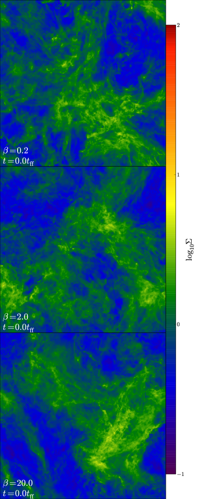
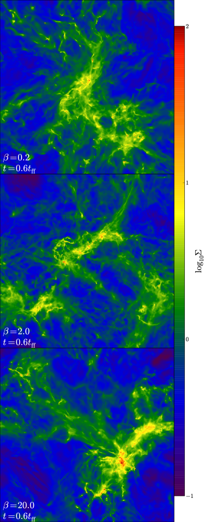
Figure 1.— Column density ($\Sigma$) for the two primary snapshots ($t=0.0t_{\rm{ff}}$, left column, and $t=0.6t_{\rm{ff}}$, right column), for all three simulations (from top to bottom, $\beta_{0}=0.2$, 2, 20, respectively). Both figures show the filamentary structure expected from both turbulence models and observations. The right column shows the addition of high density collapsing gas, and somewhat enhanced filamentary nature.

3. Density PDF

Figure 2 shows the density PDF, $V(\rho)$, for each simulation ($\beta_{0}=0.2$ in red, $\beta_{0}=2$ in green, and $\beta_{0}=20$ in blue) at $t=0.1t_{\rm{ff}}$ (solid lines) and $t=0.6t_{\rm{ff}}$ (dotted lines). This color scheme will be used throughout the paper. The figure additionally shows two grey lines that divide the gas into three sections; low density turbulent gas (left section), high density self-gravitating gas (center section), and very high density gas that is numerically unresolved (right section). The first two states are of the greatest interest to us here. The last state is interesting qualitatively, but we cannot make any quantitative measurements of the gas here. The transition density between turbulent and collapsing states, $\rho_{\rm{t}}$, is taken where the power-law begins to transition from lognormal, at $\rho_{\rm{t}}=10$. As there is likely shock-compressed gas above $\rho_{\rm{t}}$ that is not self-gravitating, $\rho_{\rm{t}}$ is not meant to be used as a phase boundary between the two states. A more complete set of criteria for the transition between turbulent and collapsing gas is currently under investigation. The second division is taken at the highest density that is still considered resolved by our refinement criterion on the finest level, as discussed in Section 2. This gives $\rho_{\rm{r}}=6347$. At this density there is also a change in the power-law slope. At very high density, corresponding to very small scale, inaccuracies in the angular momentum transport become dominant and the gas cannot collapse fully, leading to excess mass and decreased fragmentation. This can be somewhat addressed by incorporating sink particles, but as of this writing no satisfactory prescription of sink particles with magnetic fields has been developed.

In the following, we will identify the turbulent state as those features that belong to either low density gas (below $\rho_{\rm{t}}$) or gas that whose statistical properties are relatively unchanged over the course of our simulation. Collapsing gas is identified by high density (between $\rho_{\rm{t}}$ and $\rho_{\rm{r}}$) and short time variation.

3.1. Density PDF in the Turbulent State

One of the most robust properties of isothermal supersonic turbulence is the lognormal distribution of densities (Blaisdell et al. 1993; Vazquez-Semadeni 1994; Padoan et al. 1997a, b; Scalo et al. 1998; Passot & Vázquez-Semadeni 1998; Nordlund & Padoan 1999; Kritsuk et al. 2007; Federrath et al. 2008b; Price 2012). Several properties of star formation have been predicted using the lognormal distribution function, including the initial mass function (IMF) of stars (Padoan & Nordlund 2002; Padoan et al. 2007), brown dwarf frequency (Padoan & Nordlund 2004) and the star formation rate (Krumholz & McKee 2005; Padoan & Nordlund 2011).

For compressible turbulence without gravity or magnetic fields, the density PDF, $V(\rho)$, can be shown to be a lognormal of the form

$$V(\rho)d\ln\rho=\frac{1}{\sqrt{2\pi\sigma^{2}}}~{}\rm{exp}\left(\frac{(\ln\rho-\mu)^{2}}{2\sigma^{2}}\right)d\ln\rho,$$ (11)

where $\mu=-\sigma^{2}/2$ is the mean of $\ln\rho$ (Blaisdell et al. 1993; Vazquez-Semadeni 1994). The variance and Mach number, $\mathcal{M}$, are related by

$$\sigma=\sqrt{\ln(1+b^{2}\mathcal{M}^{2})}.$$ (12)

The parameter $b$ has been determined numerically to lie between 0.3 and 0.4 (Padoan et al. 1997b; Federrath et al. 2008b; Kritsuk et al. 2007; Beetz et al. 2008; Kritsuk et al. 2010a; Federrath et al. 2010). The value $b$ has been shown to approach unity in simulations with compressive forcing (Federrath et al. 2008b, 2010).

The presence of the Lorentz terms in the momentum equation breaks the invariance of the equations relative to the mean density. Thus the sequence of shocks that determine the density of a parcel of gas are no longer independent multiplicative events, as they are in hydrodynamic turbulence. For this reason there is no a priori expectation of a lognormal density distribution in a magnetized system. However, Ostriker et al. (2001) and Lemaster & Stone (2008) have shown that $V(\rho)$ is approximately lognormal, with properties weakly depending on mean field strength. For driven MHD turbulence, Lemaster & Stone (2008) find that, for densities within $10\%$ of the peak density,

$$\sigma_{\rm{LS08}}=\sqrt{|-0.72\ln\left(1+0.5\mathcal{M}^{2}\right)+0.20|},$$ (13)

and weakly decreases with field strength. Kritsuk et al. (2012, in preparation) performed high resolution simulations of statistically stationary magnetized turbulence and showed that the presence of a magnetic field alters the low density gas, making a lognormal description less appropriate. They did find that the high density wing of the PDF is still well approximated by a lognormal for the two weak field runs, $\beta_{0}=2$ and $\beta_{0}=20$.

Figure 2 shows the resemblance to a lognormal present in our simulations. In Table 1, we show $\mu$ and $\sigma$ found from fits to the average PDF for three snapshots from each of our simulations. Fits were performed for $\rho\in[5\times{10^{-3}},10]$, a range chosen to exclude material above $\rho_{\rm{t}}$. We find a weak sensitivity of $\mu$ and $\sigma$ with both time and $\beta_{0}$, with $\mu$ decreasing with time and increasing with $\beta_{0}$. Our short averaging time, relative to a dynamical time, means that these can be viewed only as snapshots in time, not as robust statistical averages.

3.2. $V(\rho)$ Collapsing State

The PDF of the collapsing material forms a power-law, $V(\rho)\propto\rho^{m}$, for densities above $\rho_{\rm{t}}$. This was first presented in hydrodynamic simulations by Klessen (2000), though the resolution of those simulations was too low to measure a significant power-law. The first measurement of the slope was done by Slyz et al. (2005), who found $m=-1.5$. This slope was also seen by Federrath et al. (2008a) and Vázquez-Semadeni et al. (2008). Kritsuk et al. (2011a) used a very high resolution AMR simulation to measure a slope of $-1.67$ at intermediate to high densities, and $-1.5$ at high density. They also provided and explanation of this power-law by comparing $V(\rho)$ to that of self-similar collapse, wherein $\rho\propto r^{n}$. The three solutions they discussed are the pressure free collapse (Penston 1969, PF), Larson-Penston supersonic infall (Larson 1969; Penston 1969, LP), and expansion wave from inside out collapse (Shu 1977, EW). Values of $n$ for various models, and the implied value of $m$, are shown in Table LABEL:table.self_similar_exponents. This table summarizes all semi-analytic and numerical results in this paper. Collins et al. (2011) measured this exponent for super-Alfvénic MHD turbulence, and found a value of $m$=$-1.64$ for $\rho\in[10,1000]$. For the simulations in this work, we find $m=-1.80,\ -1.78,$ and $-1.65$ for $\beta_{0}=0.2,\ 2$, and $20$. The $\beta_{0}=20$ case presented here is similar in both physical parameters and measured slope to that in Collins et al. (2011) and in the gas dynamic simulations of Kritsuk et al. (2011a), while the stronger field simulations show steeper values. The values found here are most consistent with the pressure-free value of $m=-1.75$.

It is clear from Figure 2 that the slope is a function of time in these clouds. This was also discussed by Kritsuk et al. (2011a). Figure 3 shows the time evolution of the power-law exponent $m$ for the last few snapshots, those that contributed to the average shown by the dashed curve in Figure 2. The two low field cases, $\beta_{0}=2$ and $20$, seem to have converged, with power-law index $m$ in the $\beta_{0}=2$ case slightly lower than the $\beta_{0}=20$ simulation. The $\beta_{0}=0.2$ simulation has clearly not converged, and is still increasing at the end of the simulation. Given the agreement of $m\approx-1.64$ between our $\beta_{0}=20$ simulation and previous simulations (Collins et al. 2011; Kritsuk et al. 2011a) and observations, we feel confident that this is a robust result in the hydrodynamic limit.

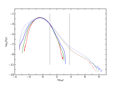
Figure 2.— Density PDF, $V(\rho)$, for each of our three-simulations, $\beta_{0}=0.2,\ 2$, and $20$ (red, green, and blue respectively), at two snapshots, $t=0.1,0.6t_{\rm{ff}}$ (solid and dotted lines, respectively). The vertical grey lines separate the low density turbulent state (left section), high density collapsing state (center section) and very high density unresolved gas (right section).

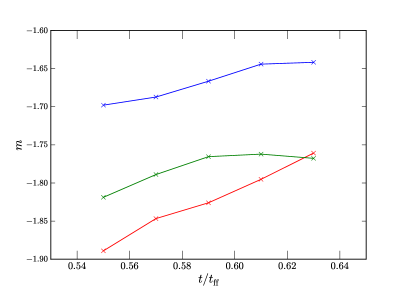
Figure 3.— The evolution of the density PDF power-law exponent, $m$, for the $\beta_{0}=0.2,\ 2,$ and $20$ simulations (red, green, and blue respectively). The value of this exponent seems to be increasing for the $\beta_{0}=0.2$ simulation, but possibly reaching a constant value for the other two.

As we will discuss in Sections 8 and 9, three dimensional compressions are suppressed with increasing magnetic field strength, as the flow is forced along magnetic field lines. This reduction in compressibility is likely the reason for the reduced value of $m$ in $\beta_{0}=2$, and delayed convergence in the $\beta_{0}=0.2$ run.

The cumulative mass fraction above some critical density $\rho_{\rm{cr}}$, defined as

$$M(\rho_{\rm{cr}})=\int_{\rho_{\rm{cr}}}^{\infty}\rho V(\rho)d\rho,$$

has been used in a number of theories of star formation, as we will discuss in Section 9.1. In order to quantify the effects of mean field, Figure 4 shows $M(\rho_{\rm{t}})$ for each run relative to the $\beta_{0}=0.2$ simulation. This shows an increase in the collapsed mass as a function of field strength. The behavior of this mass fraction with time, $M(\rho,t)$, can be used to explain the slower convergence of $m$ with the more magnetized simulations. Figure 5 shows $M(\rho_{\rm{cr}}=10,t)$, which shows that the rate at which material enters the high density state is a decreasing function of $\beta_{0}$. This can be used as a proxy for star formation, as we will discuss in Section 9.1, and while the exact rate is a function of the critical density $\rho_{\rm{c}}$, the increase of rate with $\beta_{0}$ is not.

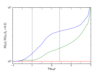
Figure 4.— Cumulative mass relative to $\beta_{0}=0.2$ case for the last snapshot, $t=0.6t_{\rm{ff}}$. Vertical lines separate turbulent (left) collapsing (center) and unresolved (right) gas.

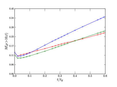
Figure 5.— Cumulative mass for $\rho>10$ vs. time for $\beta_{0}=0.2,2$, and $20$ (red, green, and blue, resepctively). This shows the rate at which gas enters the collapsing state, and is a decreasing function of $\beta_{0}$.

Table 1Lognormal Fit Parameters

	$\sigma$			$\mu$
	0.2	2.0	20	0.2	2.0	20
0.1	1.2	1.3	1.3	$-0.86$	$-0.84$	$-0.80$
0.3	1.2	1.4	1.4	$-0.97$	$-1.00$	$-1.1$
0.6	1.2	1.5	1.5	$-1.1$	$-1.2$	$-1.4$

[ sideways, star, caption = Power-law relationships, predictions, and measurements.,label=table.self_similar_exponents]l c c c c c c c c c [a]Measured values of $n$ computed from measured $m$. [b]Semi-analytic prediction of $p$ uses q=1/2. [c]Values for early and late times, respectively. Late times contain information from both turbulent and collapsing states. [d]Values for turbulent state only. [e]Values for low and high densities, respectively $\rho\propto r^{n}$ $v\propto r^{\epsilon}$ $V(\rho)\propto\rho^{m}$ $V(B)\propto B^{p}$ $P(\rho,k)\propto k^{\zeta}$ $P(\Sigma,k)\propto k^{\lambda}$ $P(v,k)\propto k^{\nu}$ $B\propto\rho^{q}$ $\beta\propto\rho^{s}$
latex rrex = $n$ urex=$\epsilon$ vrex=$m$ vbex=$p$ prex=$\zeta$ psigmaex = $\lambda$ pvex = $\nu$ brex = $q$ betarex = $s$
Index $n$ $\epsilon$ $m$= 3/$n$ $p$= $m$/$q$ $\zeta=-2(n+1)$ $-2(n+2)$ $\nu=-2(\epsilon+1)$ $q$ $s=1-2q$
LP $-2$ $0$ $-1.5$ $-3$[b] $2$ $0$ $\delta(k)$ … …
PF $-12/7$ $1/7$ $-1.75$ $-3.5$[b] $10/7$ $-4/7$ $9/7$ … …
EW $-3/2$ $-1/2$ $-2$ $-4$[b] $1$ $-1$ $0$ … …
Isotropic … … … … … … … $2/3$ $-1/3$
${\bf v}\parallel{\bf B}$ … … … … … … … $0$ $1$
${\bf v}\perp{\bf B}$ … … … … … … … $1$ $-1$
$\beta=0.2$ $-1.67$[a] … $-1.80$ $-5.4$ $-0.42,\ 0.86$[c] $-1.39,-0.11$[c] $-1.46$[d] $0.02,\ 0.43$[e] $0.96,\ 0.15$[e]
$\beta=2$ $-1.69$[a] … $-1.78$ $-4.0$ $-0.58,\ 1.12$[c] $-1.61,0.15$[c] $-1.58$[d] $0.12,\ 0.40$[e] $0.77,\ 0.19$[e]
$\beta=20$ $-1.82$[a] … $-1.65$ $-3.2$ $-0.62,\ 1.2$ [c] $-1.53,0.25$[c] $-1.80$[d] $0.23,\ 0.39$[e] $0.54,\ 0.23$[e]

4. Density Power Spectra

One of the more striking results from this study is the behavior of the density power spectrum, $P(\rho,k)$, under the effects of self-gravity. Here we have defined $P(\rho,k)$ as

$$P(\rho,k)=\sum_{|k^{\prime}|=k}\tilde{\rho}_{k^{\prime}}^{*}\tilde{\rho}_{k^{\prime}},$$ (14)

where $\tilde{\rho}$ is the Fourier transform of $\rho$, and the star denotes its conjugate. Figure 6 shows the density power spectra, $P(\rho,k)$, for all three simulations ($\beta_{0}=0.2,\ 2,$ and $20$ in red, green, and blue, respectively) at two snapshots, $t=0.1t_{\rm{ff}}$ and $t=0.6t_{\rm{ff}}$ (solid, dotted). In Figure 7 we show the power spectra for $\ln\rho$, for three snapshots of the $\beta_{0}=0.2$ simulation. Figure 8 shows the column density power spectra, $P(\Sigma,k)$. In Figures 6 and 8, the birth of the high density collapsing state can be seen in a dramatic change in the behavior of of $P(\rho,k)$, transitioning to a positive slope. This behavior is conspicuously absent in the power spectrum of the logarithm of density, as we will discuss in the following sections.

4.1. Density Power Spectra in the Turbulent State

The turbulent initial conditions can be seen in the early snapshot (solid line) in Figure 6. For weakly subsonic (but still compressible) isothermal turbulence, one expects the density to follow the pressure fluctuations, and the density power spectrum, $P(\rho,k)\propto k^{\zeta}$, should scale as $\zeta=-7/3$ (Bayly et al. 1992; Kritsuk et al. 2007). It has been seen that this power spectrum flattens with increasing Mach number. For trans-sonic turbulence, Kim & Ryu (2005) measured $\zeta=-1.7$ at a Mach number $\mathcal{M}=1.2$. For supersonic turbulence, with $\mathcal{M}=6$, Kritsuk et al. (2007) measure $\zeta=-0.9$ for a simulation with $512^{3}$ zones, and a somewhat steeper spectrum of $\zeta=-1.07$ for $1024^{3}$. For the early snapshot, we measure significantly more shallow spectra, $\zeta=-0.42,-0.58,$ and $-0.62$ for our $\beta_{0}=0.2$, 2, and 20 simulations, respectively. This fit was done for $k/k_{\rm{min}}\in[2,30]$. The flatter nature of these spectra, relative to the Kritsuk et al. (2007) work, is likely due to the higher Mach number employed in our simulations. For Burger’s equation with vanishing pressure term, which could be analogous to increasingly supersonic turbulence, Saichev & Woyczynski (1996) predict that $\zeta=0$, a trend that is consistent with $\zeta$ here being shallower than that found in Kritsuk et al. (2007). It should be noted that this comparison to Burger’s turbulence is not meant to imply that supersonic turbulence is similar to turbulence in Burger’s equation; the lack of vorticity and strong intermittency in Burger’s equation makes the two systems only superficially similar. A second potential cause of the change in slope is due to the fact that the solver employed here is more diffusive that PPM used in Kritsuk et al. (2007, 2011c), which may contribute to the change in slope. The decrease in slope with increasing magnetic field strength is consistent with the decrease in slope in the velocity power spectrum, as will be discussed in Section 7.

As discussed in Beresnyak et al. (2005), $P(\rho,k)$ is strongly influenced by the rare, high density peaks. In that work, the authors noticed that the power-spectrum of the logarithm of density was significantly steeper than $P(\rho,k)$, as the logarithm effectively filters out high density, rare peaks. This is seen in our simulations as well. The behavior of $P(\ln\rho,k)$ shows very little evolution with time, as the collapsing state is effectively filtered out, which allows us to recover the turbulent state through the entire simulation. This can be seen in Figure 7 for the $\beta_{0}=0.2$ simulation. Slopes get somewhat steeper with increasing mean field, with $\beta_{0}=0.2$ having a slope of $-1.0$, and $\beta_{0}=2$ and $20$ having slopes of $-1.4$ and $-1.53$, respectively (neither shown here).

In order to make contact with observable quantities, we show the power spectra for column density $\Sigma$, $P(\Sigma,k)\propto k^{\lambda}$, in Figure 8. For the range $k/k_{\rm{min}}\in[2,30]$ at early times, we find $\lambda=-1.39,-1.61,$ and $-1.53$ for $\beta_{0}=0.2,2$, and $20$, respectively, roughly consistent with the addition of $-1$ to $\zeta$ from the integration. Padoan et al. (2004) measured $P(\Sigma,k)$, for three star-forming clouds, Perseus, Taurus, and the Rosetta nebula. They found significantly steeper spectra than we do here, $\approx-2.8$ for all three clouds. They also performed synthetic observations through two simulations with $\mathcal{M}=10$, a super-Alfvénic simulation and an equipartition model, and find $\lambda=-2.25$ for the equipartition model and $-2.7$ for the super-Alfvénic model. The difference in slope between the slopes they found and the slopes in our simulation is most likely due to the observations and radiative transfer models missing the high density material due to the limited dynamic range, as ${}^{13}\rm{CO}$ freezes onto dust grains at densities above $10^{4}\rm{cm}^{-3}$ (Bacmann et al. 2002). As discussed in Beresnyak et al. (2005) and shown in Figure 7, the slope of the density power spectra are quite sensitive to the rare high density material, so even a slight decrease in the dynamic range of the observations will cause a steepening in the spectra. To properly compare, we will need to perform similar synthetic observations of our simulations.

4.2. Density Power Spectra in the Collapsing State

The most prominent effect of gravity is the increase in slope of $P(\rho,k)$ with time, as seen in Figure 6. For self-similar spheres with $\rho\propto r^{n}$, one finds $\zeta=-2(n+1)$. Thus, positive slopes will be seen in $P(\rho,k)$ for any $n<-1$. Expected values from different self-similar models are shown in Table LABEL:table.self_similar_exponents. Our measured values of $\zeta$ for $k/k_{\rm{min}}\in[10,200]$ are $0.86,1.12,1.2$ for $\beta_{0}$=0.2, 2, 20, respectively, at $t=0.6t_{\rm{ff}}$. Direct comparison between the measured value of $\zeta$ and those predicted from the self-similar collapse models should be handled carefully for two reasons, both stemming from to the volume weighted nature of power spectra: first, he measured value contains contributions from both the collapsing state and the turbulent state, which will tend to decrease $\zeta$ from the values expected from pure self-similar spheres; second, the power spectrum contains contributions from unresolved gas at very high densities.

The effect of increasing mean magnetic field on $P(\rho,k)$ in the collapsing state is to decrease the amount of power at all scales, increase the wavenumber at which the slope becomes positive, and slightly decreasing the slope. This is consistent with the increased compressibility and increased rate of collapse found in the more weakly magnetized simulations.

The column density power spectral slope, $\lambda$, becomes nearly flat for the collapsing case, with $\lambda=-0.11,0.15,$ and $0.25$ for $\beta_{0}=0.2,\ 2$, and $20$, respectively. This differs greatly from what is observed, owing to the fact that the material causing the flat spectra is extremely high density, with $\rho>(10^{4}-10^{8})\rho_{0}\approx(10^{6}-10^{10})\rm{cm}^{-3}$, wherein typical observational tracers such as CO are frozen onto grains, and an extremely small volume filling fraction, requiring high resolution observations. High density tracers, such as $\rm{NH}_{3}$ or deuterated species such as $\rm{H}_{2}D^{+}$, will be necessary to observe this signal (Walmsley et al. 2004; di Francesco et al. 2007). Synthetic observations of our data, as well as high resolution observations in a broad range of chemical tracers, will be required to further reconcile this discrepancy. Again, increased power with increased $\beta_{0}$ is consistent with increased compressibility of the gas.

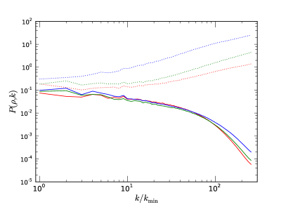
Figure 6.— Density power spectra $P(\rho,k)$ for all three simulations ($\beta_{0}$=0.2, 2, 20 colored red, green, blue) and two snapshots, $t=0.1,0.6t_{\rm{ff}}$ (solid, dotted). The increasing nature in the later snapshot is expected from self-similar spheres.

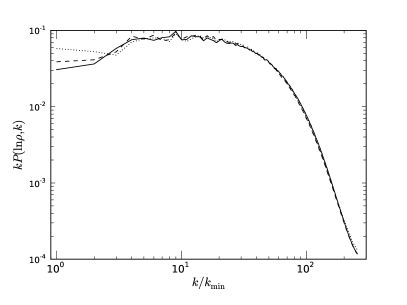
Figure 7.— Power spectra for the logarithm of density, $P(\ln\rho,k)$, for $t=0.1t_{\rm{ff}}$, $t=0.3t_{\rm{ff}}$, and $t=0.6t_{\rm{ff}}$(solid, dashed, and dotted lines) for the $\beta_{0}=0.2$ simulation. Taking the spectrum of the logarithm of density allows us to recover the turbulent state even at late times, as the collapsing state is filtered out by the logarithm. Slopes get somewhat flatter with increasing mean field; the $\beta_{0}=0.2$ simulation has a slope of $-1.0$, and the $\beta_{0}=2$ and $20$ simulations having slopes of $-1.4$ and $-1.53$, respectively (neither shown here)

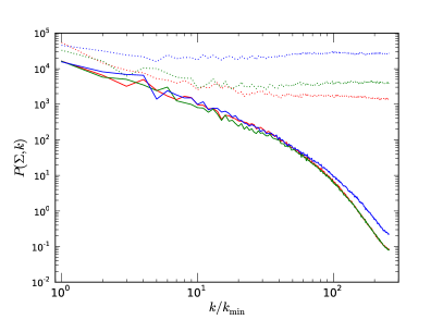
Figure 8.— Column density power spectra, $P(\Sigma,k)$. Plot style is the same as in Figure 2

5. Energy Ratios

The balance of energies sheds important light on the physical processes at play in these clouds. Figure 9 shows thermal-to-magnetic pressure ratio, $\beta_{\rm{th}}=8\pi c_{\rm{s}}^{2}\rho/B^{2}$, versus density $\rho$; and Figure 10 shows dynamic-to-magnetic pressure ratio, $\beta_{\rm{dyn}}=8\pi\rho v^{2}/B^{2}$. In both figures, the left column is taken at $t=0.1t_{\rm{ff}}$, the right from $t=0.6t_{\rm{ff}}$, and top to bottom show $\beta_{0}=0.2,\ 2$, and 20, respectively. Both figures are colored by mass fraction $F_{\rm{M}}$.

5.1. Energy Ratios in the Turbulent State

In the turbulent state, $\beta_{\rm{th}}$ shows some interesting variation with mean field. The scatter in $\beta_{\rm{th}}$ increases with increasing $\beta_{0}$, and the mean slopes in the $\beta_{\rm{th}}\propto\rho^{s}$ decreasing with increasing $\beta_{0}$; $s=0.96,\ 0.77,$ and $0.54$ for $\beta_{0}=0.2,\ 2,$ and $20$, respectively, for $\rho\in[10^{-2},10]$. The average of $\beta_{\rm{th}}$ versus $\rho$ can be seen in Figure 11. For perfectly spherical contractions, $B\propto\rho^{2/3}$, since $B\propto R^{-2}$ due to flux conservation, and $\rho\propto R^{-3}$ due to mass conservation. For flow perfectly aligned with the field, $B\propto\rho^{0}$, since no amplification of the field can take place, and for flow completely perpendicular to the field, $B\propto\rho^{1}$ (eg. Kulsrud 2004). Since $\beta_{\rm{th}}=c_{\rm{s}}^{2}\rho/B^{2}$, and for an isothermal equation of state $c_{\rm{s}}$ is constant, one finds $s=-1,\ -1/3,$ and $1$ for perpendicular, isotropic, and parallel flow, respectively. This indicates that flow is preferentially aligned in all states, even in the weakest field simulation, but the alignment increases with mean field strength

The degree to which the velocity and field are aligned is shown in Figure 12, which shows the mass weighted average of the magnitude of the cosine of the angle between ${\bf B}$ and ${\bf v}$,

$$\langle|\cos\theta|\rangle_{\rho_{\rm{i}}}=\left\langle\frac{|{\bf B}\cdot{\bf v}|}{Bv}\right\rangle_{\rho_{\rm{i}}},$$ (15)

where the average is done over only material with density in bin $\rho_{\rm{i}}$ and normalized to the total mass in that bin, and $512$ bins were used. The grey line shows the expectation value of $|\cos\theta|$ for uncorrelated vectors, $3/\pi\approx 0.64$. The solid red, green, and blue lines show $\beta_{0}=0.2,2$, and $20$, respectively, averaged for several snapshots around $t=0.6t_{\rm{ff}}.$ Light dotted lines show the constituent snapshots, which demonstrates the extremely short timescale on which $\theta$ varies at high density. The $\beta_{0}=0.2$ simulation has ${\bf B}$ and ${\bf v}$ nearly aligned at low density, which is consistent with $s=0.96\approx 1$, while the other weaker field simulations show less alignment, even a slight tendency for ${\bf B}$ and ${\bf v}$ to be perpendicular, and correspondingly lower values and larger variance in $s$.

The left column of Figure 10 shows the ratio of dynamic-to-magnetic pressure for the early snapshot. It can be seen from this figure that the typical gas element in the low-density turbulent state in the $\beta_{0}=0.2$ run is trans-Alfvén, as $\beta_{\rm{dyn}}=v^{2}/v_{\rm{A}}^{2}$ and the gas is evenly distributed around $\beta_{\rm{dyn}}=1$, with a peak of the PDF at $\beta_{\rm{dyn}}=0.54$. The other two simulations are more super-Alfvénic, with peak $\beta_{\rm{dyn}}$ at 1.2 and 5.6.

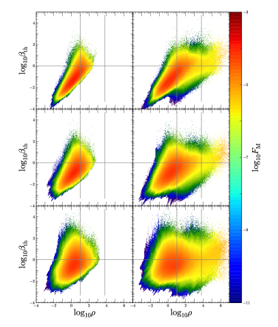
Figure 9.— Thermal-to-magnetic pressure ratio, $\beta_{\rm{th}}$, vs. $\rho$, colored by mass fraction, $F_{\rm{M}}$, at $t=t=0.1t_{\rm{ff}}$ (left column) and $t=0.6t_{\rm{ff}}$ (right columnd). Top to bottom, $\beta_{0}=0.2$,$0.2$ and $20$. Increased mean field increases the correlation between $\beta$ and $\rho$ and increasing the slope. High density gas has largely $\beta_{\rm{th}}\approx 1$, showing a tendency towards pressure balance in collapsing gas.

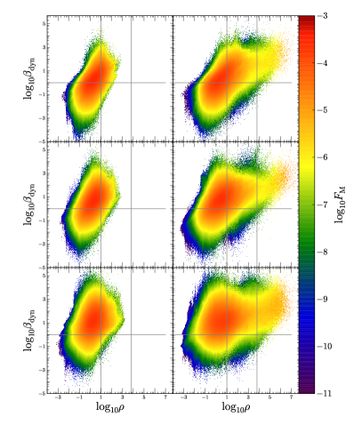
Figure 10.— Dynamic pressure ratio $\beta_{\rm{dyn}}$ for $t=0.1t_{\rm{ff}}$(left column) and $t=0.6t_{\rm{ff}}$(right column). Top to bottom, $\beta_{0}=0.2$,$0.2$ and $20$. High density gas density gas is dominated by dynamic pressure regardless of mean field strength.

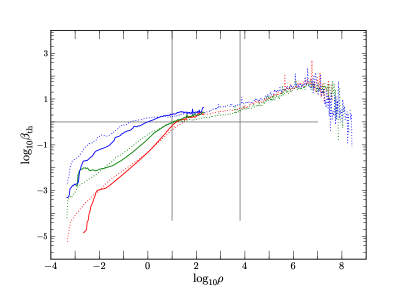
Figure 11.— Average thermal-to-magnetic pressure ratio $\beta_{\rm{th}}$ vs. $\rho$ for all three simulations, $\beta_{0}$=0.2, 2, and 20 shown in red, green, and blue respectively, at two snapshots, $t=0.1t_{\rm{ff}}$ (solid) and $t=0.6t_{\rm{ff}}$ (dotted.) The change in behavior, from turbulent to collapsing, is apparent at $\beta_{\rm{th}}\approx 1$. The horizontal line shows $\beta_{\rm{th}}=1$, and vertical lines show the three density regimes, as in Figure 2. This highlights the fact that density alone is not enough to describe the transition from turbulent to collapsing gas.

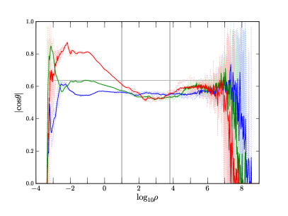
Figure 12.— Angle between ${\bf B}$ and ${\bf v}$ ($|\cos\theta|$) for a number of late-time snapshots ($t=0.57,0.59,0.61,0.63,0.65t_{\rm{ff}}$, light dotted lines) and the average (red, green, and blue for $\beta_{0}=0.2$, $\beta_{0}=2$, $\beta_{0}=20$, respectively). The horizontal line shows the expectation for random $\theta$, while the two vertical lines separate turbulent (left), collapsing (center) and unresolved (right) states.

5.2. Energy Ratios in the Collapsing State

For the high density collapsing gas, $\beta_{\rm{th}}$ and $\beta_{\rm{dyn}}$ can be seen in the right columns of Figures 9 and 10. The transition between turbulent and collapsing states is seen quite clearly in Figure 11, which shows average $\beta_{\rm{th}}$ vs. $\rho$. In this figure, at $\beta_{\rm{th}}\approx 1$ the slope in mean $\beta_{\rm{th}}$ flattens to almost zero, showing that on average, collapsing gas is in thermal-to-magnetic pressure balance. For $\rho\in[100,\rho_{\rm{r}}]$, $s=0.15,0.19,$ and $0.23$ for $\beta_{0}=0.2,2$, and $20$, respectively. A lower limit of $\rho=100$ was used for these fits as this is approximately where the slope in the $\beta_{0}=0.2$ simulation flattens dramatically. However, the density at which this transition in slope happens is found to decrease with increasing magnetic field, with $\rho\approx 10$ and $0.1$ for $\beta_{0}=2$ and $20$, respectively. This indicates that density alone is not a sufficient variable to mark the transition from turbulent to collapsing gas.

As shown in the right column of Figure 10, the collapsing gas is dominated by dynamic pressure for all three values of $\beta_{0}$. This is also true for the unresolved gas, which while one cannot quantitatively trust these results as they are contaminated by numerical resolution problems, the likelihood that increased resolution would decrease this ratio by two orders of magnitude is low. This suggests that collapsing state is formed from gas that is initially super-Alfvénic, where magnetic energy support is insufficient to resist ram pressure from the gas, causing density peaks that can become gravitationally bound. As the mass fraction of gas that is super-Alfvénic decreases with $\beta_{0}$  this also has the effect of decreasing the amount of gas that can collapse to high densities, in turn decreasing the rate and efficiency of star formation. In non-self-gravitating turbulence results, the existence of super-Alfvénic high-density gas is seen even in sub-sonic, sub-Alfvén simulations (Burkhart et al. 2009), as well as in thermally unstable trans-Alfvén simulations (Kritsuk et al. 2011b). Gravity, however, has the effect of highly concentrating the high density gas in the super-Alfvénic regime. This will be compared with observations in Section 9.

6. Magnetic Field PDF

Figure 13 shows PDF of the magnetic field for $t=0.1t_{\rm{ff}}$ (left panel) and both $t=0.1t_{\rm{ff}}$ and $t=0.6t_{\rm{ff}}$ (right panel). The left plot is linear, and shows $V(b)$, where $b$ is the fluctuating field, $b=|{\bf B}-B_{0}|$. The right plot is logarithmic, and shows the PDF for the full magnetic field $V(B)$.

6.1. Magnetic Field PDF in the Turbulent State

Kritsuk et al. (2012, in preparation) have found that the high field wing of the PDF of magnetic field in an isothermal turbulent gas can be well described by a stretched exponential, of the form

$$V(b)db=c(b^{c-1}/b_{0}^{c})\exp\left[-(b/b_{0})^{c}\right]db,$$ (16)

with a stretching exponent $c\approx 1/3$. A stretched exponential describes a sequence of multiplicative events, where $1/c$ is the depth of the hierarchy of events (Frisch & Sornette 1997; Laherrère & Sornette 1998). This is not unlike the sequence of multiplicative shocks that generates the density PDF $V(\rho)$. For $\beta_{0}=0.2$ we find $b_{0}=3.1\times{10^{-3}}$ and $c=0.33$ for $b\in[50,80]$; for $\beta_{0}=2$ we find $b_{0}=6.1\times{10^{-3}}$ and $c=0.32$, for $b\in[50,100]$; and for $\beta_{0}=20$, we find $b_{0}=9.0\times{10^{-3}}$ and $c=0.33$ for $b\in[50,120]$. Fits to these lines can be seen in black along each curve in the left panel of Figure 13 To better demonstrate the fit, Figure 14 shows $V(b)$ against $b^{1/3}$, restricted to the interval of the fit. Thus we find that the number of multiplicative events is the same for all three simulations, $1/c\approx 3$, but the characteristic scale, $b_{0}$, increases with $\beta_{0}$ due to the greater ease of inducing fluctuations in a weaker mean field.

6.2. Magnetic Field PDF in the Collapsing State

The collapsing state exhibits a power-law $V(B)\propto B^{p}$. As an example, for the mid-strength field, $\beta_{0}=2$  we find $p=-4$ for $B\in[52,530]$. This fit range was determined by the average magnetic field spanned by densities in the range $\rho\in[\rho_{\rm{t}},\rho_{\rm{r}}]$. We compute the exponent $q$ in $B\propto\rho^{q}$, and find $q=0.43$ for this simulation. Combining this with $m=-1.7$ found in Figure 3, we predict $p=-3.9$, in reasonable agreement with the measured value.

The slope of $V(B)$ increases with increasing mean field strength. For the $\beta_{0}=20$ case, we find a fit exponent $p=-3.22$ for $B\in[27,670]$, while for $\beta_{0}=0.2$ we find $p=-5.42$ for $B\in[36,451]$. Using measured values of $q$ and $m$, we predict slopes for $V(B)=-4.5,-4.0,$ and $-3.3$ for $\beta_{0}=0.2$, 2, and 20, respectively. The predicted value of $p$ for the $\beta_{0}=0.2$ run is somewhat lower than the measured value. This is likely due to the fact that the run had not yet fully developed the collapsing state.

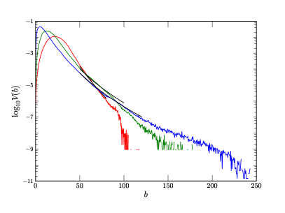
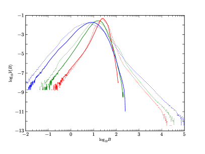
Figure 13.— PDF of magnetic field strength. (Left) PDF of fluctuating $b=|{\bf B}-B_{0}|$, $V(b)$, for $t=0.1t_{\rm{ff}}$. Fits to a stretched exponential are shown in black for each line. Note that this figure is linear in $b$. The smaller volume fractions achieved by the $\beta_{0}=20$ simulation are due to the more rapid collapse, thus earlier refinement, of that simulation. (Right) PDF of the full magnetic field strength, $B$, with lines colored the same as in Figure 2. Here we see a power-law developed at late times due to the collapsing gas. This figure illustrates how turbulence and gravity leave different signatures in the PDF of magnetic field strength; at high field strength, a stretched-exponential tail is generated by turbulence, while a power-law tail is generated by gravity.

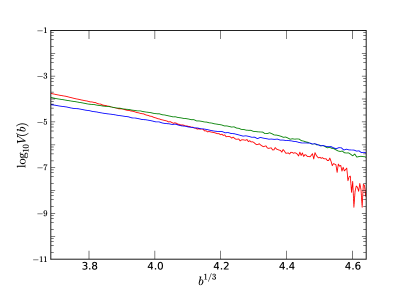
Figure 14.— The stretched exponential section of $V(b)$ at $t=0.1t_{\rm{ff}}$, restricted to the fit range $b\in[50,100]$, and plotted against $b^{1/3}$.

7. Velocity and Energy Power Spectra

The velocity power spectrum, $P(v,k)$, is historically one of the most studied quantities in turbulence modeling. Figures 15 and 16 show compensated velocity spectra. One curious feature is that the collapsing state doesn’t show up in the velocity spectra, and only shows a mild feature in the kinetic energy spectra, $P(\rho^{1/2}v,k)$, and magnetic energy spectra, $P(B,k)$, as seen in Figure 17.

7.1. Velocity and Energy Power Spectra in the Turbulent State

Only the turbulent state is visible in the velocity power spectrum, $P(v,k)$. Figure 15 shows the compensated velocity power spectra, $k^{5/3}P(v,k)$, for all snapshots for the $\beta_{0}=20$ simulation (grey lines) and the average of all snapshots (black line). The only variation comes from the first $0.1t_{\rm{ff}}$, where the variation is due entirely to the change in the effective spectral bandwidth between PPML, the solver used for the initial conditions, and the solver in Enzo, which was used for the self- gravitating AMR simulations. The rest of the snapshots, nearly indistinguishable from the mean, show almost no evolution at all. The other two simulations (not shown) show even less variation in the initial phase.

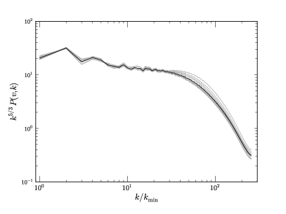
Figure 15.— Compensated velocity power spectrum $k^{5/3}P(v,k)$ for 15 snapshots between $t=0.0-0.65t_{\rm{ff}}$ for the $\beta_{0}=20$ simulation. All the evolution seen can be attributed to relaxation from the initial conditions, no evolution due to gravity is seen.

Figure 16 shows compensated power spectra for all three simulations, with red, green, and blue showing $\beta_{0}=0.2$, 2, and 20, respectively. Averages were taken over all snapshots, as the variation for $\beta_{0}=2$ and $\beta_{0}=20$ simulations were even smaller than that shown in Figure 15. Clearly, the mean field strength has a significant effect on the spectral slope. While the resolution of these simulations is too low to make precise measurements of the slope in the inertial range, measuring the slope is useful to compare scaling among the three simulations. Slopes for $k/k_{\rm{min}}\in[2,30]$ are $-1.46$, $-1.58$, and $-1.80$ for $\beta_{0}=0.2,\ 2,$ and $20$, respectively. Though there is presently no theory to predict the slope as a function of mean field in compressible MHD turbulence, the flattening of the slope with increasing mean field seen here is consistent with what one can infer from the existing theories for compressible hydro and incompressible MHD. The $\beta_{0}=20$ slope is consistent with other supersonic hydrodynamic simulation of Kritsuk et al. (2007), and is the upper end of the slope predicted by Boldyrev et al. (2002). The slope for the $\beta_{0}=0.2$ simulation is reminiscent of the $-3/2$ value of the Iroshnikov-Kraichnan model (Iroshnikov 1964; Kraichnan 1965). This reduction of slope with mean field strength was also seen by Kritsuk et al. (2009), who measure $-1.94,\ -1.62,$ and $-1.51$ for $\beta_{0}=0.2,\ 2,$ and $20$, respectively. This trend of increasing slope with mean field was continued by Lemaster & Stone (2009), who measured a slope of $-1.38$ for $\beta_{0}=0.02$, which is flatter and of lower $\beta_{0}$ than our strong field run. The $\beta_{0}=2$ run seems to be in transition between the two, with the slope increasing for wavenumbers above $k/k_{\rm{min}}=10$.

The flattening of the spectra is consistent with the magnetic energy coming into equipartition with the kinetic energy, as demonstrated by Figure 17. The magnetic energy is about ten times lower than the kinetic in the $\beta_{0}=20$ simulation for all wavenumbers, so the similarity between this run and other hydrodynamic runs is expected. The $\beta_{0}=2$ simulation displays equipartition only in a very small band around $k/k_{\rm{min}}=10$, and at higher wavenumbers, where the magnetic energy is still below equipartition, the slope of the velocity spectrum seems to increase. The $\beta_{0}=0.2$ simulation has near equipartition for the majority of the low to mid wavenumbers, and has the flattest spectrum overall.

Another illuminating feature of Figure 17 is the sub-equipartition nature of the magnetic field in these simulations at small scales at early times (solid curves). This lack of equipartition at small scales is somewhat surprising, as standard expectation of a small scale dynamo in incompressible MHD is to first grow exponentially at small scales until equipartition is reached, then linearly at larger scales, with the equipartition wavenumber decreasing with time (Brandenburg & Subramanian 2005). However, as the turbulence in this simulation is dominated by shocks, one cannot apply the same physical arguments, since the shock jump conditions do not imply simple equipartition between kinetic and magnetic energy in the shock-compressed layer. The increased fraction of kinetic energy in compressive motions (see Section 8) generates less vorticity per unit of energy than sub-sonic turbulence, which in turn generates less magnetic energy. This has been explored in Federrath et al. (2011a), who demonstrated that as Mach number increases, the ratio of magnetic to kinetic energy transitions from near unity for $\mathcal{M}<1$, to a few percent for $\mathcal{M}>1$. This is consistent with our findings here, though predominantly at small scales. In our $\beta_{0}=2$ and $\beta_{0}=0.2$ simulations, the imposed large scale field allows equipartition to be reached at intermediate scales.

7.2. Velocity and Energy Power Spectra in the Collapsing State

As seen through the time evolution of $P(v,k)$ in Figure 15, the collapse state does not leave a signature on the velocity power spectrum. This is due to the volume weighted nature of power spectra. The collapsing state occupies a very small volume fraction, as seen in Figure 2. Because of this, for a signal to appear in the power spectrum the values must be extremely large. The values of velocity reached by the gas do not vary by the many orders of magnitude that the density does in the collapsing gas, as seen in Figures 2 and 6.

If we relate the power spectra found here with the self-similar solutions discussed in Section 3.2, we find that the pressure-free collapse gives velocity scaling exponent $\nu=+5/7$; the expansion wave solution gives $\nu=0$, which gives no visible signal to the velocity scaling; finally the Larson-Penston solution, with constant velocity, gives no contribution to the velocity spectrum.

While the collapsing state leaves no signature in the velocity spectra, it does leave a signature at high $k/k_{\rm{min}}$ on the kinetic and magnetic energy spectra, $P(\rho^{1/2}v,k)$, and $P(B,k)$. In Figure 17 we show three snapshots for the energy spectrum, $P(\rho^{1/2}v,k)$ (upper set of curves) and $P(B,k)$ (lower set), for all three simulations (top to bottom, $\beta_{0}=0.2$, $\beta_{0}=2$, $\beta_{0}=20$). Solid, dashed, and dotted lines show $t=0.1,0.3,0.6t_{\rm{ff}}$, respectively. The kinetic spectrum shows an imprint of the collapse in the high $k/k_{\rm{min}}>100$ gas, due mostly to the density-weighted nature of this statistic, and the fact that, on small scales, the density increases by as much as 5 orders of magnitude. Strictly speaking, the magnetic spectrum is also a volume weighted quantity, so the increase in magnetic energy seen is a product of additional field amplification from the collapse itself. However, as discussed in Section 5, $B\propto\rho^{q}$, with $q\approx 0.4$, which is a similar to the density dependence of kinetic energy, so $P(B,k)$ can be considered to be implicitly density weighted. The initial (turbulent) field distribution is a product of the shock dominated turbulence, as discussed in the previous section. After gravity is introduced, the field sees additional amplification due to the collapse itself. This field amplification is again consistent with increased compressibility due to increased $\beta_{0}$, as the increase in $P(B)$ at high $k/k_{\rm{min}}$ is greater for the weaker field runs.

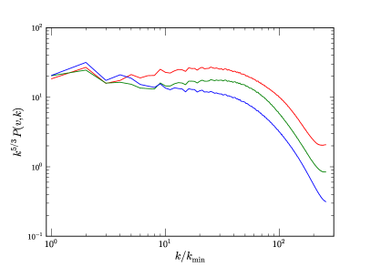
Figure 16.— Velocity power spectra $P(v,k)$ for all three simulations, averaged over all times. Slopes for $k/k_{\rm{min}}\in[2,30]$ are $-1.46$, $-1.58$, and $-1.80$ for $\beta_{0}=0.2,2,20$, respectively.

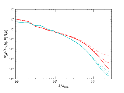
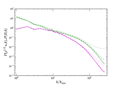
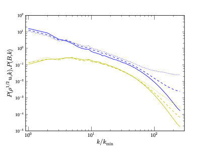
Figure 17.— Energy power spectra, $P(\rho^{1/2}v,k)$ (upper curves in each panel, red, green, and blue) and $P(B,k)$ (lower curves in each panel, cyan, magenta and yellow) for $\beta_{0}=0.2$ (top panel) $\beta_{0}=2$ (middle panel) and $\beta_{0}=20$ (bottom panel). Three different times are shown; $t=0.1t_{\rm{ff}}$ (solid line), $t=0.3t_{\rm{ff}}$ (dashed line), and $t=0.6t_{\rm{ff}}$ (dotted line)

If one examines the energy scaling in the context of self-similar spheres, one finds that $P(\rho^{1/2}u)$ scales as $k^{+1}$ for the Larson-Penston and pressure-free solutions, and $k^{+3/7}$ for the expansion wave solutions. These increasing solutions are not seen in Figure 17. Again this is likely due to the fact that the superposition of the turbulent and collapsing spectra makes distinguishing between the two difficult.

8. Helmholtz Decomposisition

The formation of high density material necessarily comes from compressive motions. A standard method of examining the compressional and solenoidal modes of the velocity field is the Helmholtz decomposition. We split the velocity field, ${\bf v}$, into two components

$${\bf v}={\bf v_{c}} +{\bf v_{s}},$$ (17)

$$\nabla\cdot{\bf v_{s}} =0,$$ (18)

$$\nabla\times{\bf v_{c}} =0,$$ (19)

where we find ${\bf v_{c}}$ and ${\bf v_{s}}$ in Fourier space,

$$\tilde{{\bf v}}_{\rm{c}} =(\hat{k}\cdot\tilde{{\bf v}})\hat{k},$$ (20)

$$\tilde{{\bf v}}_{\rm{s}} =\tilde{{\bf v}}-\tilde{{\bf v}}_{\rm{c}}$$ (21)

where $\tilde{{\bf v}}$ is the Fourier component of ${\bf v}$, and $\hat{k}$ is the unit wave vector. We then examine the ratio of the power spectra $\chi(k)=P({{\bf v_{c}}},k)/P({{\bf v_{s}}},k)$, which gives us a scale-wise measure of the importance of compressibility of the gas.

8.1. Helmholtz Decomposition in the Turbulent State

The ratio of compressible to solenoidal power, $\chi(k)$, is shown in Figure 18 for the same fiducial snapshots as in Figure 2. For $\beta_{0}=20$, we find $\chi(k)\approx 0.4$ in the range $k/k_{\rm{min}}\in[2,30]$, which is less than $0.5$ as expected from purely geometrical considerations: for a given wave vector $\bf{k}$ there is only one longitudinal (compressional) component, while there are two transverse (rotational) components. This is consistent with the findings of Kritsuk et al. (2010b), where the increase of the magnetic field strength decreases $\chi(k)$. Again we find the increased compressibility with increased $\beta_{0}$. At low $k/k_{\rm{min}}<50$ there is a monotonic increase in $\chi(k)$ with $\beta_{0}$. The $\beta_{0}=20$ simulation also shows a substantial low $k/k_{\rm{min}}<2$ compression at late times, seen to a lesser extent in the other two. The $\beta_{0}=2$ run shows a peak in $\chi(k)$ at $k/k_{\rm{min}}\approx 10$, probably with a similar origin as the $k/k_{\rm{min}}<2$ increases, namely a result of the large scale forcing pattern. In all cases, there is a general trend of increasing compressibility at higher $k/k_{\rm{min}}$. As discussed in Section 7, this increase in compressibility causes reduced amplification of the magnetic field at high $k/k_{\rm{min}}$.

8.2. Helmholtz Decomposition in the Collapsing State

There is no substantial increase in compressive motions at high $k/k_{\rm{min}}$ as time progresses, indicating, as for the velocity power spectrum, $P(v,k)$, that this statistic is not especially sensitive to gravity, due to its volume-weighted nature. It seems that the lower levels of magnetization in the $\beta_{0}=20$ simulation is enough for that run to have some increased compressional motion at high $k/k_{\rm{min}}$. The stronger field runs show almost no evolution. At low $k/k_{\rm{min}}$, all three simulations show an increase in power at $k/k_{\rm{min}}<2$. This is possibly due to the effects of gravity causing large scale contraction of the gas.

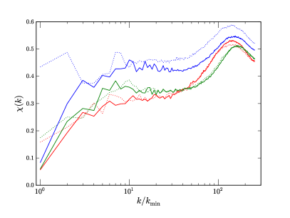
Figure 18.— The ratio of compressible to solenoidal motions, $\chi(k)=P({\bf v_{c}},k)/P({\bf v_{s}},k)$, for all three simulations (red, green and blue for $\beta_{0}=0.2$, $\beta_{0}=2$, $\beta_{0}=20$) and two snapshots ($t=0.1,0.6t_{\rm{ff}}$, solid and dotted lines, respectively)

9. Discussion

The combined effects of gravity, turbulence, and magnetic fields have yet to be incorporated in star formation theory with their proper respective weights. Here we discuss modifications to two recent star formation models (Section 9.1) and interpret several recent observations in this light (Section 9.2).

9.1. Implications on Theory

In the past decade, the lognormal density PDF of turbulence has been used to predict a number of properties of star formation, including the star formation rate. Here we will examine the implication on two works in particular, namely the star formation rate models of Krumholz & McKee (2005), hereafter KM05, and Padoan & Nordlund (2011), hereafter PN11. In both of these works, the star formation rate per free fall time, $\rm{SFR_{ff}}$, is predicted to be proportional to the mass fraction above some critical density, using a lognormal distribution. Thus

$$\rm{SFR_{ff}} =\epsilon\int_{\rho_{\rm{cr}}}^{\infty}\rho V(\rho)d\rho$$ (22)

$$=\epsilon\left(1+\rm{erf}\left[\frac{\sigma^{2}-2\ln\rho_{\rm{cr}}}{2^{3/2}\sigma}\right]\right),$$ (23)

where we have used Equation 11 in the derivation of the second of these. This model presumes that the effects of gravity do not alter the structure of the star-forming cloud. However if the effects of gravity are present during the formation of the cloud, it is not unreasonable to suppose that a power-law density PDF might be present before the onset of turbulence. Here we will explore what effects the distribution may have on the star formation rate.

KM05 and PN11 differ in two ways: the nature of $\epsilon$ and the nature of $\rho_{\rm{cr}}$. The parameter $\epsilon$ contains the timescale for collapse, as well as the fraction of collapsing gas reaching the proto-star. The other difference is the nature of $\rho_{\rm{cr}}$. In KM05, $\rho_{\rm{cr}}$ is the density at which velocity perturbations become subsonic and lose their turbulent support. In PN11, $\rho_{\rm{cr}}$ is the post shock density that yields clumps that are larger than the sum of the Bonnor-Ebert and magnetic critical masses.

As we have shown in Section 7, the scaling of the turbulence depends on the mean magnetic field. This in turn has consequences for the expected critical density. The KM05 result predicts that

$$\rho_{\rm{cr}}=\left(\phi\frac{\lambda_{\rm{J}}}{\lambda_{\rm{s}}}\right)^{2},$$ (24)

$$\lambda_{s}=L_{0}(c_{\rm{s}}/\sigma_{0})^{1/q},$$ (25)

thus

$$\rho_{\rm{cr}}=\left(\phi\frac{\lambda_{\rm{J}}}{L_{0}}\right)^{2}\mathcal{M}^{2/q}$$ (26)

where $\lambda_{\rm{s}}$ is the sonic length, at which velocity perturbations become subsonic, $L_{0}$ is the cloud size, $\sigma_{0}$ is the velocity fluctuation at the outer scale, and $\phi$ is a numerical factor of order unity. In their work they find $\phi=1.12$. We can relate $q$ to the velocity spectral index $\nu$ by $q=-(\nu+1)/2$. For $\nu=-2$, as expected for pressure free turbulence, $q=1/2$, while for $\nu=-1.5$ as seen in our $\beta_{0}=0.2$ run, $q=1/4$. If we take $\mathcal{M}=10$, we find an increase of several orders of magnitude in $\rho_{\rm{cr}}$ when using the spectral scaling of the $\beta_{0}=0.2$ simulation over the $\beta_{0}=20$ simulation, assuming everything else stays constant. In PN11, $\rho_{\rm{cr}}$ does not depend directly on $\nu$, but will likely impact the post-shock magnetic field distribution, similarly increasing $\rho_{\rm{cr}}$ for increasing mean field strength.

Another impact of our results here is the result of replacing the turbulent PDF, $V(\rho)$, with one that transitions to a power-law at some transition density $\rho_{t}$. Thus,

$$V_{\rm{p}}(\rho)d\ln\rho=\begin{cases}N\frac{1}{\sqrt{2\pi}\rho\sigma}\rm{exp}\left[\frac{(\ln\rho-\mu)^{2}}{2\sigma^{2}}\right]d\ln\rho,&\rho<\rho_{\rm{t}}\\ N\rho_{0}\rho^{m}d\ln\rho,&\rho>\rho_{\rm{t}},\end{cases}$$ (27)

rather than a plain lognormal. Here the normalization $N$ is determined by the normalization requirement, $\int_{-\infty}^{\infty}V_{\rm{p}}(\rho)d\ln\rho=1$, and is given by

$$N=2\left(1+\rm{erf}\left(\frac{2\ln\rho_{\rm{t}}+\sigma^{2}}{2^{3/2}\sigma}\right)-\frac{2\rho_{0}\rho_{\rm{t}}^{m}}{m}\right)^{-1}.$$ (28)

From here we are left to determine the critical density for star formation, $\rho_{\rm{cr}}$, and the density at which the PDF transitions from lognormal to power-law, $\rho_{\rm{t}}$. These are not necessarily equal; the forces of rotation and magnetic fields will suppress the collapse of material once the gas is within the potential well of the self-similar sphere, whereby $\rho_{\rm{cr}}$ may be larger than $\rho_{\rm{t}}$. If we assume that $V(\rho)$ is continuous and differentiable, we can piece together an analytic estimate for $\rho_{0}$ and $\rho_{\rm{t}}.$ Differentiability is not necessarily the correct condition to take, but in the absence of a better condition for the transition density $\rho_{\rm{t}}$, an assumption must be made. The PDF in Figure 2 as well as some observations do appear to be differentiable. Nevertheless, we can use this assumption to examine the sensitivity of $\rm{SFR_{ff}}$ to $\rho_{\rm{t}}$ and $\rho_{0}$. These two conditions give us

$$\rho_{\rm{t}} =\frac{1}{2}(2m-1)\sigma^{2}$$ (29)

$$\rho_{0} =e^{\sigma^{2}m(m-1)/2}.$$ (30)

Using the fit values from Table 1, we find values listed in Table LABEL:table.transition_fits. We also compute values for the Larson-Penston sphere, with $\rho\propto r^{-2}$ and $\sigma=1.5$ as found for the majority of our simulations, and a pressure-free collapse with $\sigma$ taken from Equation 12 for $b=0.4$ and $\mathcal{M}=9$.

The increase in predicted star formation rate is found by using this piecewise PDF instead of a lognormal in Equation 23. In Figure 19, we plot the piecewise cumulative mass fraction in Equation 27 relative to the purely lognormal mass fraction versus critical density $\rho_{\rm{cr}}$. We have used parameters from all three simulations, red, green, and blue lines for $\beta_{0}=0.2,\ 2$, and $20$, respectively, the Larson-Penston solution in black, and the pressure free solution in grey. We find that the increase in star formation rate can be quite large, and is quite sensitive to the details of $\rho_{\rm{t}}$ and $m$. This clearly predicts the incorrect behavior in rate relative to $\beta_{0}$, as the $\beta_{0}=0.2$ model has a measured collapse rate lower than the other two (see Figure 5) . This is due to the selection of $\rho_{\rm{t}}$, which is significantly lower for $\beta_{0}=0.2$ than the other two, caused by the lower value of $\sigma$. While this is an incorrect prediction, it demonstrates how sensitive this type of model is to the parameters of the fit. In reality, $\rho_{\rm{cr}}$ and $\rho_{\rm{t}}$ will be functions of a stability criterion that fully incorporates magnetic fields and turbulence.

This result is consistent with the findings of Cho & Kim (2011), who used $512^{3}$ unigrid simulations to examine the collapse rate for various values of critical density. For the largest critical values, $\rho_{\rm{cr}}=500\rho_{0}$, they find an increase of 2400 relative to the predicted value of KM05.

Future work will analyze bound clumps to determine a proper value for $\rho_{\rm{cr}}$ and $\rho_{\rm{t}}$, and further evaluate this prediction as well as KM05 and PN11.

[pos=h,caption=Parameters for extended density PDF,label=table.transition_fits]ccccc model $m$ $\sigma$ $\rho_{0}$ $\rho_{\rm{t}}$

0.2 1.2 1.75 2.4 6

2 1.5 1.75 3.2 17

20 1.5 1.64 2.4 13

PF 1.8 1.71 3.4 24

LP 1.5 1.5 1.9 10

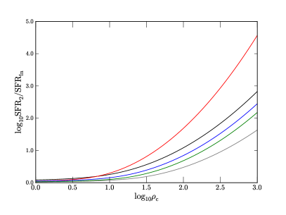
Figure 19.— Excess cumulative mass fraction of a power-law PDF relative to a lognormal PDF. This gives the amount by which the two primary star formation rate models are low. The black line uses $\sigma=1.5,m=-1.5,\rho_{0}=0.5$. Red, green, and blue lines use $\sigma$ taken from Table 1, $m$ from Figure 3, and $\rho_{0}$ from Equation 30. The grey line uses a pressure-free solution (PF)

One question that is not addressed by this work is when star formation begins in the lifetime of a cloud. That is, are the effects of self gravity already present before the lognormal PDF is established, in which case a power-law $V(\rho)$ is the best picture to take, or is a star-forming cloud turbulent first, and then transitions to self-gravitating through cooling? Kainulainen et al. (2009) two families of clouds, one with only lognormal PDFs and no star formation, and one family that includes power-law tails and high rates of star formation. However it is presently unknown if the star formation begins before or after the power-law tail, or if the tail impacts the star formation itself.

9.2. Interpretation of Observations

The role of magnetic fields has been vigorously debated over the last few decades. Initially magnetic fields were the dominant mechanism for regulating star formation (Mouschovias 1976; Shu et al. 1987), then relegated to an insignificant role as supersonic turbulence took hold (Mac Low & Klessen 2004; Krumholz & McKee 2005). Recent observations have given a mixed review of the role of magnetic fields, with some measurements indicating a strong field, and some indicating a weak field. Here we will discuss the implications of our present model on recent observations.

Li et al. (2009) measured starlight polarization in a number of molecular clouds, and averaged said polarization over large (30 pc) scales of the cloud and small (0.3 pc) scales centered on high density cloud cores. The resultant alignment of magnetic fields on large and small scales is interpreted to imply sub-Alfvénic  magnetic fields, by way of comparison to a set of super-Alfvénic ($\mathcal{M_{\rm{A}}}=2$) and sub-Alfvénic ($\mathcal{M_{\rm{A}}}=0.7$) simulations. In sub-Alfvénicturbulence, the kinetic energy of the gas is unable to alter the alignment of the magnetic field at all scales, leading to alignment with the mean field at all scales and a correlation between direction at both large and small scales. In contrast, super-Alfvénic turbulence can greatly alter the magnetic field direction, reducing the correlation between large and small scales. This is consistent with the increase in mean alignment between ${\bf v}$ and ${\bf B}$ with decreasing $\beta_{0}$ (Figure 12), as in our trans-Alfvénic simulation there is a trend towards alignment that is absent from the higher $\beta_{0}$ runs. In our trans-Alfvénic simulation, kinetic energy is insufficnent to alter the direction of the field relative to the mean, and in turn velocity and magnetic vectors are aligned. In the super-Alfvénic simulations, on the other hand, kinetic motions dominate and the field direction can be altered by the velocity. On the other hand, recent measurements of the directions of outflow from T-Tauri stars are uncorrelated with mean magnetic field (Ménard & Duchêne 2004; Targon et al. 2011), though there is a weak correlation for earlier Class 0 and Class 1 objects (Targon et al. 2011). Finally, two sets of observational papers show a transition in field strength with scale. Crutcher et al. (2010) find that density is uncorrelated with field strength for densities $n_{\rm{H}}<10^{3}$, and correlated as $B\propto n^{0.65}$ for higher densities, using Zeeman splitting. Heyer & Brunt (2012) use velocity anisotropy in the Taurus molecular cloud to show that the low column density gas, with more anisotropic flows, is likely trans-Alfvénic, while high column density gas, with more isotropic flow, is likely super-Alfvénic.

This suite of measurements is consistent with what we have seen in this study, and can be understood by the combination of Figures 10, 12, and 17, focusing on the $\beta_{0}=0.2$ simulation. Through the action of supersonic turbulence, the effect of magnetic fields is a function of scale. Low $k/k_{\rm{min}}$ gas, where the turbulence is generated in the presence of an appreciable mean field, comes into equipartition. This allows low density gas to exhibit alignment seen in observations. However in material at higher $k/k_{\rm{min}}$, where the structures are generated by shocks, the field is unable to come into equipartition. This high density gas is further selected to be super-Alfvénic in post-shock gas where the magnetic energy is too weak to resist compression.

We also find that our simulations are filled with filamentary structures, as seen by Men’shchikov et al. (2010) with Hershel in the Aquila and Polaris clouds, see Figures 1 and 20. Figure 20 shows a restricted region of the $t=0.6t_{\rm{ff}}$ snapshot of the $\beta_{0}=2$ simulation, overlaid with magnetic field vectors (right panel) and velocity vectors (left panel). High density material, with $\rho>10$, is nearly all concentrated in filamentary structures, as seen in Arzoumanian et al. (2011). Further analysis is necessary to quantify the filament width distribution, as in that work filaments cluster tightly around $0.1\rm{pc}$. Magnetic fields are weak and perpendicular to the structure with the cores, while in the lower density filamentary tail the field is parallel to the structure. This is expected by the fact that all high density material is super-Alfvénic: the filament aligned with the magnetic field will have maximally amplified the magnetic field, halting the collapse, while the material with ${\bf B}$ and ${\bf v}$ more closely aligned has lower supporting pressure due to the reduced field amplification, and can go on to form “stars”.

We can make further contact between the collapsing state and observations of prestellar cores seen in the Aquila star-forming cloud, as reported by André et al. (2010). We can estimate the mass-size relation from a self-similar sphere as

$$M(R)=4\pi\int_{0}^{R}\rho(r)r^{2}dr\propto R^{n+3}$$ (31)

which gives us $M(r)\propto r^{1}$ for the LP solution, $M(r)\propto r^{1.3}$ for the PF solution (see also Kritsuk & Norman (2011)). The value found in Aquila is 1.13 (Philippe André, private communication.), which is somewhat shallower than that of the LP solution. For completeness, the expansion wave solution predicts $M(r)\propto r^{1.5}$, though is less relevant due to the fact that the expansion wave solution presupposes a central singularity, while the André result focused on starless cores.

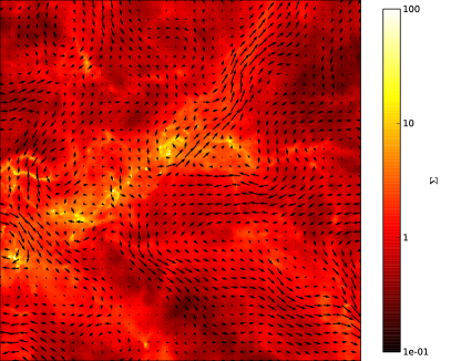
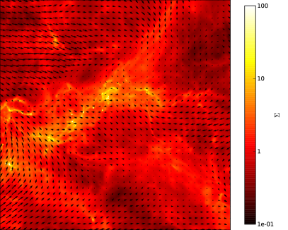
Figure 20.— Projections of a sub set of dense gas from the $\beta_{0}=2$ simulation at $t=0.6t_{\rm{ff}}$. Overlaid are magnetic vectors (left) and velocity vectors (right). The dense parts of this filament lie at the convergence of opposing velocity streams, where the magnetic field is roughly aligned to the velocity. Higher in the stream, where the field is perpendicular to the velocity, collapse is suppressed.

10. Conclusions

In this work, we use high resolution AMR MHD simulations to examine the combined effects of self-gravity and magnetic fields on supersonic turbulence. We find that self-gravity bifurcates the cloud into two phases: a low density, turbulent cloud; and high density, self-gravitating cores. The two phases have substantially different statistical properties. The magnetic field serves to effectively decrease compressibility of the gas as the mean magnetic field is increased.

The simulations were performed using the AMR Enzo code (Bryan et al. 1995; O’Shea et al. 2004), extended to MHD by Collins et al. (2010). The three simulations use an rms Mach number $\mathcal{M}=9$, virial parameter $\alpha=1$, and three values of the mean magnetic field, giving initial plasma beta $\beta_{0}=0.2,2,20$. The coarse level had $512^{3}$ zones, and 4 levels of refinement were used, refining to keep the Jeans length resolved by 16 zones. This gives an effective resolution of $8196^{3}$.

The low density turbulent state exhibits properties anticipated by earlier works in supersonic hydro and MHD turbulence The effects of increasing mean magnetic field strength are to decrease both the compressibility and the ability of the gas flow to bend field lines. The properties of the turbulent state can be summarized as follows:

• Density PDF, $V(\rho)$, can be roughly represented by a lognormal, given by Equation 11. The width of the lognormal increases somewhat with increasing mean thermal-to-magnetic pressure ratio, $\beta_{0}$.

• The density power spectrum, $P(\rho,k)\propto k^{\zeta}$, tends to flatten with increasing Mach number. We find slopes that are flatter than other measurements of $\zeta$ in supersonic turbulent simulations, in proportion to the higher Mach number relative to earlier work. We find that $\zeta$ weakly decreases with increasing $\beta_{0}$. For the early snapshot, $\zeta=-0.42,-0.58,$ and $-0.62$ for $\beta_{0}=0.2,\ 2$, and $20$, respectively;

• The column density power spectrum, $P(\Sigma,k)\propto k^{\lambda}$, is also flatter than observed. We find $\lambda=-1.39,-1.61,$ and $-1.53$ for $\beta_{0}=0.2,\ 2$, and $20$, respectively, while values of $\lambda<-2.25$ have been reported elsewhere. This discrepancy is likely due to the decreased density range in earlier measurements, in part due to the reduced dynamic range available to the single tracer molecules used for the observations.

• Thermal-to-magnetic pressure ratio, $\beta_{\rm{th}}$, shows a decreasing correlation between $\beta_{\rm{th}}$ and $\rho$ with increasing $\beta_{0}$. The average slope also decreases with decreasing field. For $\beta_{\rm{th}}\propto\rho^{s}$, $s=0.97,\ 0.77,$ and $0.54$ for $\beta_{0}=0.2,\ 2$, and $20$, respectively.

• Dynamic-to-magnetic pressure ratio, $\beta_{\rm{dyn}}$, shows only mild decrease in correlation between $\beta_{\rm{dyn}}$ and $\rho$, and the peak of the distribution decreases with increasing $\beta_{0}$.

• The magnetic field and velocity are nearly aligned for mid- to low-density gas in the strong field case, and decorrelated for the other two cases.

• the PDF of magnetic field, $V(b)\propto\exp[-(b/b_{0})^{c}]$, shows a stretched exponential with a stretching exponent of $c\approx 1/3$, as given in Equation 16, for the high field strength gas. The slope decreases with $\beta_{0}$, with $b_{0}=0.15,0.19$ and $0.23$ for $\beta_{0}=0.2,\ 2$, and $20$, respectively, and the peak decreases with increasing $\beta_{0}$.

• The velocity power spectra, $P(v,k)\propto k^{\nu}$, show an increasing slope as $\beta_{0}$ increases, with the weak field case resembling supersonic hydrodynamic turbulence; we find that $\nu=-1.46,\ -1.58$, and $-1.80$ for $\beta_{0}=0.2,\ 2$, and $20$, respectively.

• Equipartition between kinetic and magnetic energy is only seen at large scale for the strongest field case, $\beta_{0}=0.2$, and a small range of intermediate wavenumbers for $\beta_{0}=2$; the magnetic energy is an order of magnitude or more for all high wavenumbers in all simulations, and all wavenumbers in the weak-field case, $\beta_{0}=20$.

• The ratio of compressive-to-solenoidal motions, $\chi(k)$, increases with $\beta_{0}$, indicating increased compressibility with decreased magnetic field strength.

The high-density collapse phase exhibits properties consistent with spherically symmetric isothermal collapse solutions, with power-law density profiles $\rho\propto r^{n}$. Again the effect of the magnetic field is to decrease the compressibility of the gas. The properties of the collapsing state can be summarized as follows:

• The density PDF is well approximated by a power-law, $V(\rho)\propto\rho^{m}$, where $m=3/n$, and $m=-1.80,\ -1.78,$ and $-1.65$ for $\beta_{0}=0.2,\ 2$, and $20$, respectively. The mass flux rate, which can be seen as a proxy for star formation rate, is an increasing function of $\beta_{0}$. The slope in the strong field case is continuing to increase at the end of the simulation, due to the slower collapse in this case.

• The density power spectrum, $P(\rho,k)\propto k^{\zeta}$, shows a positive slope, consistent with the expected behavior of a self-similar solution, $\zeta=-2(m+1)$, though detailed comparison to theory is difficult due to the superposition of the turbulent state. We find that $\zeta=0.86,1.12$, and $1.2$ for $\beta_{0}=0.2,\ 2$, and $20$, respectively.

• The column density spectrum $P(\Sigma,k)\propto k^{\lambda}$, shows flat spectra, with $\lambda\approx 0$ for all simulations; this behavior is potentially observable, provided observational tracers with high enough dynamic range are used.

• The thermal-to-magnetic pressure ratio, $\beta_{\rm{th}}$, is near unity for all values of $\beta_{0}$.

• The dynamic-to-magnetic pressure ratio, $\beta_{\rm{dyn}}$, is larger than unity by at least two orders of magnitude for all values of $\beta_{\rm{dyn}}$.

• The high density gas shows a decrease in the mean alignment between ${\bf B}$ and ${\bf v}$ with increasing density.

• The magnetic field PDF shows a power-law behavior, $V(B)\propto B^{p}$, with $p=-5.42,-4,$ and $-3.22$ for $\beta_{0}=0.2,\ 2$, and $20$, respectively.

• The velocity power spectra show no evidence of the collapsing state, due to the small volume fraction of the collapsing gas and lack of severe increase in velocity, as seen in the density power spectrum.

• The kinetic energy spectra, $P(\rho^{1/2}u,k)$, and $P(B,k)$ show increases in power at high $k/k_{\rm{min}}$, consistent with the density weighted nature of these two statistics.

• The ratio of compressive-to-solenoidal power similarly shows almost no signature of the collapsing state.

We find that for certain values of the transition from lognormal to power-law density PDF, the feedback on the predicted star formation rate can be quite large. This has sensitive dependence on the transition density, $\rho_{\rm{t}}$ between lognormal to power-law, and the critical density, $\rho_{\rm{cr}}$, above which cores are considered to be gravitationally bound. Additionally the flattening of the velocity power spectrum in the trans-Alfvénic simulation will cause high density material to remain gravitationally bound to smaller scales, increasing $\rho_{\rm{cr}}$ from values expected from hydrodynamic scaling.

High density collapsing gas is created very super-Alfvénic, with $\mathcal{M_{\rm{A}}}\approx 100$, even in the trans-Alfvénic simulation. In the trans-Alfvénic simulation, we find large scale imprints of the magnetic field, and at small scale this imprint weakens. This is consistent with a number of recent observations of the properties of star-forming clouds. High density cores seem to be found primarily in filaments, in regions where the magnetic field is aligned perpendicular to the filament. Filaments with longitudinal magnetic fields do not show high density material, consistent with the super-Alfvénic nature of the collapsing state being a necessary condition for collapse.

This work was supported in part by the National Science Foundation under grants AST0808184 and AST0908740; D.C., H.L. and H.X. were supported in part by Los Alamos National Laboratory, LLC for the National Nuclear Security Administration of the U.S. Department of Energy under contract DE-AC52-06NA25396. A.K. was supported in part by the National Science Foundation grant AST-1109570. H.L. gratefully acknowledges the support of the U.S. Department of Energy through the LANL/LDRD program. Computer time was provided through NSF TRAC allocations TG-AST090110 and TG-MCA07S014. The computations were performed on Nautilus and Kraken at the National Institute for Computational Sciences (http://www.nics.tennessee.edu/).

References

- REV (????)
- 08 (1)
- André et al. (2010) André, P., Men’shchikov, A., Bontemps, S., et al. 2010, A&A, 518, L102
- Arzoumanian et al. (2011) Arzoumanian, D., André, P., Didelon, P., et al. 2011, A&A, 529, L6
- Bacmann et al. (2002) Bacmann, A., Lefloch, B., Ceccarelli, C., et al. 2002, A&A, 389, L6
- Balsara (2001) Balsara, D. S. 2001, J. Comput. Phys, 174, 614
- Bayly et al. (1992) Bayly, B. J., Levermore, C. D., & Passot, T. 1992, Phys. Fluids A, 4, 945
- Beetz et al. (2008) Beetz, C., Schwarz, C., Dreher, J., & Grauer, R. 2008, Phys. Lett. A, 372, 3037
- Beresnyak et al. (2005) Beresnyak, A., Lazarian, A., & Cho, J. 2005, ApJ, 624, L93
- Berger & Colella (1989) Berger, M. J., & Colella, P. 1989, J. Comput. Phys, 82, 64
- Blaisdell et al. (1993) Blaisdell, G. A., Mansour, N. N., & Reynolds, W. C. 1993, J. Fluid Mech., 256, 443
- Boldyrev et al. (2002) Boldyrev, S., Nordlund, Å., & Padoan, P. 2002, ApJ, 573, 678
- Brandenburg & Subramanian (2005) Brandenburg, A., & Subramanian, K. 2005, Phys. Rep., 417, 1
- Bryan et al. (1995) Bryan, G. L., Norman, M. L., Stone, J. M., Cen, R., & Ostriker, J. P. 1995, Comput. Phys. Commun., 89, 149
- Burkhart et al. (2009) Burkhart, B., Falceta-Gonçalves, D., Kowal, G., & Lazarian, A. 2009, ApJ, 693, 250
- Cho & Lazarian (2003) Cho, J., & Lazarian, A. 2003, MNRAS, 345, 325
- Cho & Kim (2011) Cho, W., & Kim, J. 2011, MNRAS, 410, L8
- Collins et al. (2011) Collins, D. C., Padoan, P., Norman, M. L., & Xu, H. 2011, ApJ, 731, 59
- Collins et al. (2010) Collins, D. C., Xu, H., Norman, M. L., Li, H., & Li, S. 2010, ApJS, 186, 308
- Crutcher et al. (2010) Crutcher, R. M., Wandelt, B., Heiles, C., Falgarone, E., & Troland, T. H. 2010, ApJ, 725, 466
- di Francesco et al. (2007) di Francesco, J., Evans, II, N. J., Caselli, P., et al. 2007, Protostars and Planets V, 17
- Dobbs et al. (2011) Dobbs, C. L., Burkert, A., & Pringle, J. E. 2011, MNRAS, 413, 2935
- Dolag & Stasyszyn (2009) Dolag, K., & Stasyszyn, F. 2009, MNRAS, 398, 1678
- Elmegreen (1993) Elmegreen, B. G. 1993, ApJ, 419, L29
- Federrath et al. (2011a) Federrath, C., Chabrier, G., Schober, J., et al. 2011a, Phys. Rev. Lett., 107, 114504
- Federrath et al. (2008a) Federrath, C., Glover, S. C. O., Klessen, R. S., & Schmidt, W. 2008a, Physica Scripta Volume T, 132, 014025
- Federrath et al. (2008b) Federrath, C., Klessen, R. S., & Schmidt, W. 2008b, ApJ, 688, L79
- Federrath et al. (2010) Federrath, C., Roman-Duval, J., Klessen, R. S., Schmidt, W., & Mac Low, M. 2010, A&A, 512, A81
- Federrath et al. (2011b) Federrath, C., Sur, S., Schleicher, D. R. G., Banerjee, R., & Klessen, R. S. 2011b, ApJ, 731, 62
- Frisch & Sornette (1997) Frisch, U., & Sornette, D. 1997, J. Phys., 7, 1155
- Fromang et al. (2006) Fromang, S., Hennebelle, P., & Teyssier, R. 2006, A&A, 457, 371, ramses
- Gaburov & Nitadori (2011) Gaburov, E., & Nitadori, K. 2011, MNRAS, 414, 129
- Galli & Shu (1993) Galli, D., & Shu, F. H. 1993, ApJ, 417, 220
- Gardiner & Stone (2005) Gardiner, T. A., & Stone, J. M. 2005, J. Comput. Phys, 205, 509
- Goldreich & Sridhar (1995) Goldreich, P., & Sridhar, S. 1995, ApJ, 438, 763
- Goodman et al. (2009) Goodman, A. A., Rosolowsky, E. W., Borkin, M. A., et al. 2009, Nature, 457, 63
- Heyer et al. (2009) Heyer, M., Krawczyk, C., Duval, J., & Jackson, J. M. 2009, ApJ, 699, 1092
- Heyer & Brunt (2012) Heyer, M. H., & Brunt, C. M. 2012, MNRAS, 420, 1562
- Heyer et al. (2001) Heyer, M. H., Carpenter, J. M., & Snell, R. L. 2001, ApJ, 551, 852
- Iroshnikov (1964) Iroshnikov, P. S. 1964, Soviet Astronomy, 7, 566
- Kainulainen et al. (2009) Kainulainen, J., Beuther, H., Henning, T., & Plume, R. 2009, A&A, 508, L35
- Kim & Ryu (2005) Kim, J., & Ryu, D. 2005, ApJ, 630, L45
- Klessen (2000) Klessen, R. S. 2000, ApJ, 535, 869
- Kraichnan (1965) Kraichnan, R. H. 1965, Phys. Fluids, 8, 1385
- Kritsuk & Norman (2011) Kritsuk, A. G., & Norman, M. L. 2011, arXiv:1111.2827
- Kritsuk et al. (2007) Kritsuk, A. G., Norman, M. L., Padoan, P., & Wagner, R. 2007, ApJ, 665, 416
- Kritsuk et al. (2011a) Kritsuk, A. G., Norman, M. L., & Wagner, R. 2011a, ApJ, 727, L20
- Kritsuk et al. (2011b) Kritsuk, A. G., Ustyugov, S. D., & Norman, M. L. 2011b, in IAU Symposium, Vol. 270, Computational Star Formation, ed. J. Alves, B. G. Elmegreen, J. M. Girart, & V. Trimble, 179–186
- Kritsuk et al. (2009) Kritsuk, A. G., Ustyugov, S. D., Norman, M. L., & Padoan, P. 2009, in ASP Conf. Ser., Vol. 406, Numerical Modeling of Space Plasma Flows: ASTRONUM-2008, ed. N. V. Pogorelov, E. Audit, P. Colella, & G. P. Zank (San Fransisco: ASP), 15
- Kritsuk et al. (2010a) Kritsuk, A. G., Ustyugov, S. D., Norman, M. L., & Padoan, P. 2010a, in ASP Conf. Ser., Vol. 429, Numerical Modeling of Space Plasma Flows: ASTRONUM-2009, ed. N. V. Pogorelov (San Fransisco: ASP), 15
- Kritsuk et al. (2010b) Kritsuk, A. G., Ustyugov, S. D., Norman, M. L., & Padoan, P. 2010b, in Astronomical Society of the Pacific Conference Series, Vol. 429, Numerical Modeling of Space Plasma Flows, Astronum-2009, ed. N. V. Pogorelov, E. Audit, & G. P. Zank, 15
- Kritsuk et al. (2011c) Kritsuk, A. G., Nordlund, Å., Collins, D., et al. 2011c, ApJ, 737, 13
- Krumholz & McKee (2005) Krumholz, M. R., & McKee, C. F. 2005, ApJ, 630, 250
- Kulsrud (2004) Kulsrud, R. 2004, Plasma Physics for Astrophysics (Princeton University Press)
- Laherrère & Sornette (1998) Laherrère, J., & Sornette, D. 1998, European Physical Journal B, 2, 525
- Larson (1969) Larson, R. B. 1969, MNRAS, 145, 271
- Larson (1981) —. 1981, MNRAS, 194, 809
- Lemaster & Stone (2008) Lemaster, M. N., & Stone, J. M. 2008, ApJ, 682, L97
- Lemaster & Stone (2009) —. 2009, ApJ, 691, 1092
- Li et al. (2009) Li, H.-b., Dowell, C. D., Goodman, A., Hildebrand, R., & Novak, G. 2009, ApJ, 704, 891
- Li et al. (2008) Li, S., Li, H., & Cen, R. 2008, ApJS, 174, 1
- Mac Low (1999) Mac Low, M.-M. 1999, ApJ, 524, 169
- Mac Low & Klessen (2004) Mac Low, M.-M., & Klessen, R. S. 2004, Rev. Mod. Phys. , 76, 125
- Ménard & Duchêne (2004) Ménard, F., & Duchêne, G. 2004, A&A, 425, 973
- Men’shchikov et al. (2010) Men’shchikov, A., André, P., Didelon, P., et al. 2010, A&A, 518, L103
- Mestel & Spitzer (1956) Mestel, L., & Spitzer, Jr., L. 1956, MNRAS, 116, 503
- Mignone (2007) Mignone, A. 2007, J. Comput. Phys, 225, 1427
- Mouschovias (1976) Mouschovias, T. C. 1976, ApJ, 207, 141
- Nordlund & Padoan (1999) Nordlund, Å. K., & Padoan, P. 1999, in Interstellar Turbulence, ed. J. Franco & A. Carraminana, 218
- O’Shea et al. (2004) O’Shea, B. W., Bryan, G., Bordner, J., et al. 2004, arXiv:astro-ph/0403044
- Ostriker et al. (2001) Ostriker, E. C., Stone, J. M., & Gammie, C. F. 2001, ApJ, 546, 980
- Padoan et al. (2004) Padoan, P., Jimenez, R., Juvela, M., & Nordlund, Å. 2004, ApJ, 604, L49
- Padoan et al. (1997a) Padoan, P., Jones, B. J. T., & Nordlund, A. P. 1997a, ApJ, 474, 730
- Padoan & Nordlund (2002) Padoan, P., & Nordlund, Å. 2002, ApJ, 576, 870
- Padoan & Nordlund (2004) —. 2004, ApJ, 617, 559
- Padoan & Nordlund (2011) —. 2011, ApJ, 730, 40
- Padoan et al. (1997b) Padoan, P., Nordlund, A., & Jones, B. J. T. 1997b, MNRAS, 288, 145
- Padoan et al. (2007) Padoan, P., Nordlund, Å., Kritsuk, A. G., Norman, M. L., & Li, P. S. 2007, ApJ, 661, 972
- Passot & Vázquez-Semadeni (1998) Passot, T., & Vázquez-Semadeni, E. 1998, Phys. Rev. E, 58, 4501
- Penston (1969) Penston, M. V. 1969, MNRAS, 144, 425
- Price (2012) Price, D. J. 2012, J. Comput. Phys, 231, 759
- Price & Bate (2008) Price, D. J., & Bate, M. R. 2008, MNRAS, 385, 1820
- Price & Monaghan (2004) Price, D. J., & Monaghan, J. J. 2004, MNRAS, 348, 123
- Saichev & Woyczynski (1996) Saichev, A. I., & Woyczynski, W. A. 1996, SIAM J. Appl. Math., 56, 1008
- Scalo et al. (1998) Scalo, J., Vazquez-Semadeni, E., Chappell, D., & Passot, T. 1998, ApJ, 504, 835
- Scott & Black (1980) Scott, E. H., & Black, D. C. 1980, ApJ, 239, 166
- Shu (1977) Shu, F. H. 1977, ApJ, 214, 488
- Shu et al. (1987) Shu, F. H., Adams, F. C., & Lizano, S. 1987, ARA&A, 25, 23
- Slyz et al. (2005) Slyz, A. D., Devriendt, J. E. G., Bryan, G., & Silk, J. 2005, MNRAS, 356, 737
- Targon et al. (2011) Targon, C. G., Rodrigues, C. V., Cerqueira, A. H., & Hickel, G. R. 2011, ApJ, 743, 54
- Turk et al. (2011) Turk, M. J., Smith, B. D., Oishi, J. S., et al. 2011, ApJS, 192, 9
- Ustyugov et al. (2009) Ustyugov, S. D., Popov, M. V., Kritsuk, A. G., & Norman, M. L. 2009, J. Comput. Phys, 228, 7614
- Vazquez-Semadeni (1994) Vazquez-Semadeni, E. 1994, ApJ, 423, 681
- Vázquez-Semadeni et al. (2008) Vázquez-Semadeni, E., González, R. F., Ballesteros-Paredes, J., Gazol, A., & Kim, J. 2008, MNRAS, 390, 769
- Walmsley et al. (2004) Walmsley, C. M., Flower, D. R., & Pineau des Forêts, G. 2004, A&A, 418, 1035