An additive version of Ramsey’s theorem

Abstract

We show that, for every $r,k$, there is an $n=n(r,k)$ so that any $r$-coloring of the edges of the complete graph on $[n]$ will yield a monochromatic complete subgraph on vertices $\left\{a+\sum_{i\in I}d_{i}\mid I\subseteq[k]\right\}$ for some choice of $a,d_{1},\ldots,d_{k}$. In particular, there is always a solution to $x_{1}+\ldots+x_{\ell}=y_{1}+\ldots+y_{\ell}$ whose induced subgraph is monochromatic.

1 Introduction

Given a set $X$ and a number $r$, an $r$-coloring of $X$ is any map $\chi:X\rightarrow[r]$, where $[r]=\{1,\ldots,r\}$ is the set of colors.

Ramsey’s celebrated theorem [8] states that, given $r,k$, there is an $R=R(r,k)$ so that any $r$-coloring of the edges of the complete graph on $R$ vertices contains a monochromatic complete graph on $k$ vertices. In addition to being an important result in itself, Ramsey is the namesake of a large field of research into Ramsey Theory, which more generally tells when a coloring of a large structure is guaranteed to have large monochromatic substructures. There are many great resources on Ramsey Theory, but the main source is due to Graham, Rothschild, and Spencer [3].

The first result in Ramsey theory was actually proved by Hilbert in 1892, predating Ramsey’s theorem (1930) by several decades. Given natural numbers $a,d_{1},\ldots,d_{k}$, define

$$H(a;d_{1},\ldots,d_{k})=\left\{a+\sum_{i\in I}d_{i}\mid I\subseteq[k]\right\}.$$

We call such a set $H(a;d_{1},\ldots,d_{k})$ a Hilbert cube of dimension $k$. Hilbert proved [5] that, given $r,k$ natural numbers, there is a number $H=H(r,k)$ so that any $r$-coloring of $[H]$ contains a monochromatic Hilbert cube of dimension $k$.

It was further shown that finite-colorings of natural numbers would always contain monochromatic solutions to $x+y=z$ (Schur [9]), as well as long monochromatic arithmetic progressions (van der Waerden [11]). The holy grail of results of this type is Rado’s theorem [7], which characterizes which systems of linear equations have monochromatic solutions under every finite-coloring of the naturals. Those which do are called partition-regular.

These results are philosophically related to Ramsey’s theorem, but the graph theoretic and additive sides of Ramsey theory are largely distinct fields. In recent years, however, Deuber, Gunderson, Hindman, and Strauss proved a connecting result [1] — for any $m$, any sufficiently large graph either contains a $K_{m,m}$, or else it has an independent set with a prescribed additive structure. Later, Gunderson, Leader, Prömel, and Rödl showed [4] that for any $m,k$, large graphs must either contain a $K_{m}$ or there must be an arithmetic progression of length $k$ which is an independent set. There have been further results in this area, but none give a purely additive result.

Our goal is to find some additive property $\mathcal{P}$ for which we can guarantee that every finite edge-coloring of the complete graph on $[n]$ will contain a set of vertices with property $\mathcal{P}$ whose induced subgraph is monochromatic. In this paper, we consider properties where $X$ has property $\mathcal{P}$ if $X$ satisfies a particular system of linear equations.

We always demand solutions by distinct values, so that the monochromatic subgraphs are non-trivial. For example, if we solve $x+y=z$ by $x=y=3,z=6$, the corresponding graph has only a single edge, $\{3,6\}$. The induced graph has no choice but to be monochromatic.

Formally, given a matrix $B$ and a number of colors $r$, we would like to know whether there is an $n=n(r,B)$ so that any $r$-edge-coloring of the complete graph on $[n]$ gives a vector $\vec{x}=(x_{1},\ldots,x_{k})$ of distinct entries so that the values $\{x_{1},\ldots,x_{k}\}$ are monochromatic, and $B\vec{x}=\vec{0}$.

We consider this problem for many systems of equations known to be partition-regular. In Section 2, we give several negative results. In Section 3 we give an initial positive result: there is an $n$ so that, any 2-coloring of the edges of the complete graph on $[n]$ gives a monochromatic 2-dimensional Hilbert cube. In Section 4, we prove a lemma about coloring $k$-ary trees which may be interesting on its own. In Section 5 we extend our initial result to any number of colors and to Hilbert cubes of any size. We believe these are the first explicit positive results in this direction.

2 Negative results

There are many families of equations for which monochromatic solutions can be easily avoided in this graph setting.

2.1 Arithmetic progressions

Van der Waerden’s theorem [11] tells us that any finite-coloring of the naturals have arbitrarily long monochromatic arithmetic progressions. What can we say when coloring pairs of naturals? An arithmetic progression of length 3 is given by $a,a+d,a+2d$. We notice that the triple contains two differences: $d$ and $2d$. This observation allows us to 2-color the complete graph on the naturals without a monochromatic 3-AP.

The coloring is simple. For a pair $\{x,y\}$, write $|x-y|=2^{p}q$ where $p,q$ are integers and $q$ is odd. If $p$ is even, color $\{x,y\}$ red. Otherwise, color it blue.

Now let $a,a+d,a+2d$ be a 3-AP. Write $d=2^{p}q$. Then we see $2d=2^{p+1}q$, so the edges $\{a,a+d\}$ and $\{a,a+2d\}$ have different colors.

This coloring avoids 3-APs, so we certainly cannot hope for anything longer.

2.2 Schur’s equation and generalizations

Schur’s theorem [9] states that any finite-coloring of the naturals has a mono-chromatic solution to $x+y=z$. Additionally, it follows from Folkman’s theorem that there is a monochromatic solution to $x_{1}+\ldots+x_{k}=z$ for arbitrary $k$.

More generally, we consider equations of the form

$$a_{1}x_{1}+\ldots+a_{k}x_{k}=bz$$ (1)

with $a_{1},\ldots,a_{k}\geq b>0$.

We note that any solution to Equation 1 has $x_{i}\leq z$ for $i=1,\ldots,k$. Using two colors, we can ensure that every graph induced by a solution to an equation of this form in the natural numbers contains both colors. We first show how to avoid $x+y=z$ as motivation for the approach, and then handle the general case.

If $x+y=z$ then either $x$ or $y$ is smaller than their average, $\frac{1}{2}z$, and the other must be larger than their average. Thus, given a pair $\{u,v\}$ with $u<v$, we color it red if $u\leq\frac{1}{2}v$, and blue if $u>\frac{1}{2}v$. Now we see that whenever $x+y=z$, the largest of the three numbers must be $z$. Either $x$ or $y$ is smaller than $\frac{1}{2}z$, and the other is larger, so the pairs $\{x,z\}$ and $\{y,z\}$ have different colors. (Recall that we are only interested in solutions by distinct numbers).

In Equation 1, a similar logic applies. We see that $a_{i}x_{i}\leq bz$. Since $a_{i}\geq b>0$, we get $x_{i}\leq z$ as before. Let $M=a_{1}+\ldots+a_{k}$. Divide both sides of the equation by $M$ to get

$$\frac{a_{1}}{M}x_{1}+\ldots+\frac{a_{k}}{M}x_{k}=\frac{b}{M}z.$$

This says that the weighted average of the $x_{i}$’s is $\frac{b}{M}z$. Again, one of the $x_{i}$’s must be smaller than their average, and another must be larger. Thus, when $u<v$, we should color $\{u,v\}$ red if $u\leq\frac{b}{M}v$, and blue otherwise. We immediately see that one of the pairs $\{x_{i},z\}$ must be red and another must be blue.

Remark:

The argument given above is really a greedy coloring. At step $t$, color the pairs $\{1,t\},\ldots,\{t-1,t\}$ in a way that handles those solutions to Equation 1 with largest element $t$. Since we can manage all these solutions at once, we avoid all monochromatic solutions. The incredible thing to notice here is that this coloring is much stronger than needed. If $x_{1},\ldots,x_{k},z$ satisfy Equation 1, then the star connecting $z$ to all of the $x_{i}$’s is not even monochromatic. Forget about the clique! The strength of this technique suggests that we may be able to handle a larger family of equations.

On the other hand, this technique relies heavily on the numbers being positive. If we change the underlying set to $\mathbb{Z}$ or $\mathbb{Z}_{p}$, the approach falls apart.

2.3 Three variables, six colors

As with many problems in Ramsey theory, we may consider our conjecture as a hypergraph coloring problem. The vertex set is all pairs we are considering (be they pairs in $[n],\mathbb{N},\mathbb{Z},\mathbb{Z}_{n}$, etc). For each solution $(x_{1},\ldots,x_{k})$ to $b_{1}x_{1}+\ldots+b_{k}x_{k}=0$, there is a hyperedge containing all pairs of the $x_{i}$’s. If we properly color this $\binom{k}{2}$-uniform hypergraph (avoiding monochromatic hyperedges), then there are no monochromatic solutions to the equation. Thus we may apply theorems about hypergraph coloring.

For an equation in three variables, this hypergraph is simple — any two pairs are either disjoint (and have no hyperedges in common), or have the form $\{x,y\},\{x,z\}$, leaving only $\{y,z\}$ to form a hyperedge.

Fix $a,b,c$, and consider the hypergraph formed as above by the equation

$$ax+by+cz=0.$$ (2)

Consider a pair $\{u,v\}$. How many hyperedges can it be contained in? Well, there are 6 different ways of assigning the values $u$ and $v$ to the variables in Equation 2:

$$\begin{array}[]{rcl}au+bv+cz=0&\implies&z=-\frac{au+bv}{c}\\ av+bu+cz=0&\implies&z=-\frac{av+bu}{c}\\ au+by+cv=0&\implies&y=-\frac{au+cv}{b}\\ av+by+cu=0&\implies&y=-\frac{av+cu}{b}\\ ax+bu+cv=0&\implies&x=-\frac{bu+cv}{a}\\ ax+bv+cu=0&\implies&x=-\frac{bv+cu}{a}\\ \end{array}$$

Thus we see that, so long as the numbers $a,b,c$ are all invertible, each pair $\{u,v\}$ is contained in at most 6 hyperedges. In particular, if we are in $\mathbb{Z},\mathbb{Q}$, or $\mathbb{Z}_{p}$ for a prime $p$, then the degree is at most 6. The hypergraph version of Brooks’ theorem [6] applies.

Theorem 2.1.

If $H$ is a hypergraph with maximum degree $\Delta$, then $\chi(H)\leq\Delta$ except in these cases:

1. $\Delta=1$,

2. $\Delta=2$ and $H$ contains an odd cycle (an ordinary graph),

3. $H$ contains a $K_{\Delta}$ (an ordinary graph).

Since all of these cases are irrelevant — ours is a 3-uniform hypergraph, and we don’t have any illusions that we can 1-color it — this tells us we can properly 6-color our hypergraph. By construction, this avoids monochromatic solutions to Equation 2.

Moreover, if for example $a=b$, then the six solutions reduce to three distinguishable ones, meaning 3 colors is enough.

Note 2.2.

We avoided considering solutions over $\mathbb{Z}_{n}$ with $n$ composite and $a,b,c$ not necessarily invertible. Taken to extremes, this case is quite degenerate. Consider, for example, $n=2^{r}$, and $a=b=2^{r-1}$. Any collection of even numbers then solves Equation 2. The problem of finding a solution which induces a monochromatic subgraph now reduces to the multicolor Ramsey’s theorem for triangles.

3 Two colors, two dimensions

We will eventually prove the following result:

Theorem 3.1.

For all $r,k$, there is a number $n=n(r,k)$ so that any $r$-coloring of the edges of the complete graph on $[n]$ gives a Hilbert cube $H=H(a;d_{1},\ldots,d_{k})$ so that all edges in $H$ are the same color, and the $2^{k}$ elements of $H$ are distinct.

We first prove the theorem for $r=k=2$. Note that a 2-dimensional Hilbert cube is four numbers of the form $a,a+b,a+c,a+b+c$. We will then extend those ideas to any number of colors, and then to Hilbert cubes of any dimension.

The proof will rely on the Gallai-Witt theorem [12], and a consequence of Rado’s theorem [7], both of which we state here.

Theorem 3.2 (Gallai-Witt).

For all $r,k$, there exists $GW=GW(r,k)$ so that any $r$-coloring of $[GW]\times[GW]$ gives numbers $x,y,d$ with the property that

$$\left\{(x+id,y+jd)\mid i,j=0,\ldots,k-1\right\}$$

are all the same color.

Theorem 3.3 (Corollary to Rado).

There is a number $T$ so that any 2-coloring of $[T]$ gives distinct numbers $i,j,i+j,j-i$, all the same color.

Note: Rado’s theorem gives conditions for a system of linear equations to have monochromatic solutions by distinct numbers. It is a simple exercise to check that the above satisfies them.

Proof of Theorem 3.1 when $r=k=2$.

Define $S=GW(T+1,2)$, where $T$ comes from Theorem 3.3. We will show that $n=2S$ suffices.

Fix an $2$-coloring $\chi:\binom{[n]}{2}\rightarrow[2]$. We would like to find a solution to $w+x=y+z$ which forms a monochromatic clique. We view $\chi$ as a coloring of the upper half of the lattice $[n]\times[n]$ — for $x<y$, the color of $(x,y)$ is $\chi(\{x,y\})$.

Consider the top left quadrant of our grid: $\{1,\ldots,S\}\times\{S+1,\ldots,2S\}$. Define $\chi^{\prime}:[S]\times[S]\rightarrow[2]$ by

$$\chi^{\prime}(a,b)=\chi(a,S+b).$$

Since $S=GW(T+1,2)$, and $\chi^{\prime}$ is a $2$-coloring of $[S]\times[S]$, we may apply Gallai-Witt to find $x,y,d$ so that all points of the form

$$\{(x+id,y+jd)\mid i,j=0,\ldots,T\}$$

are the same color, say red, under $\chi$. We will consider each subsquare of this large grid.

For now, consider a red square given by the points

$$(a,b)\quad(a+h,b)\quad(a,b+h)\quad(a+h,b+h).$$

We may rewrite the underlying numbers as $a,a+h,a+(b-a),a+h+(b-a)$ to see they form a Hilbert cube of dimension 2.

There are six edges in the graph on these four numbers, and we know that four of them are red. Thus, we only need to consider the edges $\{a,a+h\}$ and $\{b,b+h\}$. If these are both red (and the four values are distinct), then we have the desired monochromatic 4-clique. Thus, either we have our goal, or every red square gives us two edges which cannot both be red.

Well, we have a great many red squares. Each has corner $(x+id,y+jd)$ and side-length $\ell d$, for every choice of $i,j,\ell$ with $i,j,i+\ell,j+\ell$ all in $\{0,\ldots,S\}$. The four underlying numbers are all distinct by the choice of our initial grid $\{1,\ldots,S\}\times\{S+1,\ldots,2S\}$. The “final” edges of this square are $\{x+id,x+(i+\ell)d\}$ and $\{y+jd,y+(j+\ell)d\}$, so these two cannot both be red without reaching our goal.

All of our red squares will give us many interacting conditions, which we record in a graph. Let $G=(A\cup B,E)$ be a bipartite graph, where $A=B=\binom{\{0,\ldots,T\}}{2}$. We say $\{a,a^{\prime}\}\sim\{b,b^{\prime}\}$ if $\{x+ad,x+a^{\prime}d\}$ and $\{y+bd,y+b^{\prime}d\}$ are the final edges of some red square. There is an induced 2-coloring of both $A$ and $B$ — namely

$$\chi_{A}(\{i,j\})=\chi(x+id,x+jd),$$

$$\chi_{B}(\{i,j\})=\chi(y+id,y+jd)$$

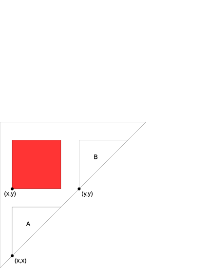
Figure 1: A large red grid, and the corresponding sets $A$ and $B$

We see immediately that $\{i,i+\ell\}\sim\{j,j+\ell\}$ so long as those numbers are all in $\{0,\ldots,T\}$. This means that each pair in $A$ with difference $\ell$ is connected to every pair in $B$ with that difference. This means that if one pair in $A$ is red, all pairs in $B$ with that difference must be blue (and vice versa). In fact, this is the entire structure of $G$.

Write $A=A_{1}\cup A_{2}\cup\ldots\cup A_{T}$, where $A_{\ell}$ contains all pairs in $A$ of the form $\{i,i+\ell\}$. We now 2-color $[T]$, the index set of the $A_{\ell}$’s. Say $\phi(\ell)=\hbox{red}$ if any pair in $A_{\ell}$ is red. Otherwise, $\phi(\ell)=\hbox{blue}$, meaning that $A_{\ell}$ is entirely blue. Since $\phi$ is a 2-coloring of $[T]$, Theorem 3.3 tells us there are distinct numbers $i,j,i+j,j-i$ which are monochromatic.

Case 1: The numbers are red. This means each set $A_{i},A_{j},A_{i+j},A_{j-i}$ contains a red pair. Therefore the corresponding sets in $B$, what we should call $B_{i},B_{j},B_{i+j},B_{j-i}$, are all entirely blue. The proof continues as in case 2 below, but with all $A$’s changed to $B$’s, and all $x$’s changed to $y$’s.

Case 2: The numbers are blue, so all pairs in $A_{i},A_{j},A_{i+j},A_{j-i}$ are blue. We list the relevant blue pairs:

$$\begin{array}[]{rl}\hbox{In }A_{i}:&\{0,i\},\{j,i+j\}\\ \hbox{In }A_{j}:&\{0,j\},\{i,i+j\}\\ \hbox{In }A_{i+j}:&\{0,i+j\}\\ \hbox{In }A_{j-i}:&\{i,i+(j-i)\}=\{i,j\}.\end{array}$$

Taken together, we see that $0,i,j,i+j$ form a blue $K_{4}$ under $\chi_{A}$. Recalling the relationship between $\chi$ and $\chi_{A}$, this gives us a blue $K_{4}$ under $\chi$ with vertices $x,x+id,x+jd,x+(i+j)d$. This is the desired 2-dimensional Hilbert cube. ∎

4 Coloring $k$-ary trees

In order to achieve Theorem 3.1 for any number of colors, we will first require a Ramsey-type theorem for $k$-ary trees.

Notation 4.1.

We use $[k]^{*}$ to denote all finite sequences (strings) of elements of $[k]=\{1,\ldots,k\}$. If $s,t\in[k]^{*}$, we use $s\cdot t$ to denote concatenation — all characters of $s$ followed by all characters of $t$.

Def 4.2.

A perfect $k$-ary tree $T_{n}^{(k)}$ of height $n$ is the collection of nodes

$$T_{n}^{(k)}=\{s\in\{1,\ldots,k\}^{j}\mid 0\leq j\leq n\}.$$

We say $\lambda$, the empty string, is the root of the tree. A node $s$ has $k$ children, $s\cdot 1,\ldots,s\cdot k$. The child $s\cdot i$ together with all of its descendants forms the $i^{\hbox{th}}$ subtree of $s$, rooted at $s\cdot i$. We see that $s$ has $k$ subtrees in all. The $j^{\hbox{th}}$ level of $T_{n}^{(k)}$ consists of all those strings of length exactly $j$. The substrings of $s$ are called the ancestors of $s$. The nodes at level $n$ are called leaves. If $s$ is a substring of $t$, we say that the path from $s$ to $t$ is the set of nodes $r$ which are both superstrings of $s$ and substrings of $t$ (including $s$ and $t$). The length of the path is the difference in lengths of $s$ and $t$.

Since we are only interested in perfect $k$-ary trees in this paper, we will usually refer to them simply as “$k$-ary trees”, or “trees” if $k$ is implied.

Next, we define what it means to embed one $k$-ary tree into another.

Def 4.3.

Let $T,R$ be two $k$-ary trees. An embedding of $T$ into $R$ is a map $\varphi$ from the nodes of $T$ into the nodes of $R$ with the following properties:

1. There is an increasing function $x$ from levels of $T$ to levels of $R$ so that, if $t$ is on the $i^{\hbox{th}}$ level of $T$, then $\varphi(t)$ is on the $x(i)^{\hbox{th}}$ level of $R$.

2. If $s,t$ are nodes in $T$ , and $s$ is contained in the $i^{\hbox{th}}$ subtree of $t$, then $\varphi(s)$ is contained in the $i^{\hbox{th}}$ subtree of $\varphi(t)$.

We now state the goal of this section:

Lemma 4.4.

For every $k,c,n$, there is a number $E=E(k,c,n)$ so that every $c$-coloring of the $k$-ary tree of height $E$ yields a monochromatic embedding of the $k$-ary tree of height $n$.

We say that a coloring is $n$-balanced if the conclusion holds.

Example 4.5.

A coloring $\chi$ of the a tree $T$ is 1-balanced if there is some node $r$, and strings $s_{1},\ldots,s_{k}\in[k]^{j}$ for some $j$, so that

$$r,r\cdot 1\cdot s_{1},\ldots,r\cdot k\cdot s_{k}$$

are all the same color. This corresponds to the embedding $\varphi$ of $T_{1}^{(k)}$ into $T$ given by $\varphi(\lambda)=r,\varphi(i)=r\cdot i\cdot s_{i}$.

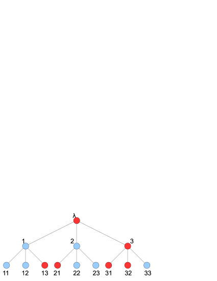
Figure 2: This 3-ary tree is 1-balanced. The nodes $\lambda$, 13, 21, and 31 are all red

We prove Lemma 4.4 by first finding $f(k,c)=E(k,c,1)$, and repeatedly applying that result.

Lemma 4.6.

There is a function $f(k,c)$ so that, if $n\geq f(k,c)$, then every $c$-coloring of the perfect $k$-ary tree of depth $n$ is 1-balanced.

We take the proof slowly to delicately handle each part.

Proof.

When $c=1$ the nodes $\lambda,1,2,\ldots,k$ must all be the same color, so they 1-balance the tree. Thus $f(k,1)=1$.

Consider the case $k=1$, so that each level has a unique node. By the pigeonhole principle, the $c+1$ nodes within levels $0,1,\ldots,c$ must contain two with the same color. Thus $f(1,c)=c$.

We begin the same way for $k=2$. Since we know $f(2,1)=1$, we work by induction on $c$. We will show $f(2,c+1)\leq(c+1)(1+f(2,c))$. Call this number $n$.

Let $\chi:T_{n}^{(2)}\rightarrow[c+1]$ be a $(c+1)$-coloring of the tree of height $n$. Consider the path from the root to the node $1^{n}$. The path contains $n+1$ nodes, so some color is represented at least

$$\left\lceil\frac{n+1}{c+1}\right\rceil=2+f(2,c)$$

times. Call the repeated color “red.” Call the levels of these red nodes $j(-1),j(0),j(1),\ldots,j(f(2,c))$. Since we looked down the path of all 1s, the corresponding nodes are

$$\begin{array}[]{rcl}r&=&1^{j(-1)}\\ s_{0}&=&1^{j(0)}\\ &\vdots&\\ s_{f(2,c)}&=&1^{j(f(2,c))}.\\ \end{array}$$

Consider $r$ along with any of the other red nodes, $s_{i}$. These may be part of a balancing triple — if any descendent $t$ of $r\cdot 2$ on level $j(i)$ is also red, then $r,s_{i},t$ balance the tree. Thus, if the tree is to be unbalanced, all of the levels $j(0),\ldots,j(f(2,c))$ within the second subtree of $r$ must be entirely non-red. We will now use the definition of $f(2,c)$ to show that this tree is in fact 1-balanced by these non-red nodes.

Consider the map from the nodes of $T=T_{f(2,c)}^{(2)}$ into our tree given by

$$\varphi(\lambda)=r\cdot 2^{j(0)-j(-1)}=1^{j(-1)}\cdot 2^{j(0)-j(-1)},$$

$$\varphi(a_{1}\ldots a_{\ell-1}a_{\ell})=\varphi(a_{1}\ldots a_{\ell-1})\cdot(a_{\ell})^{j(\ell)-j(\ell-1)}.$$

We make the following observations:

1. Nothing in the image of $\varphi$ is red (unless the coloring is 1-balanced).

2. All nodes on level $i$ of $T$ are mapped to level $j(i)$ of our tree.

3. If $t$ is contained in the $i^{\hbox{th}}$ subtree of $s$, then $\varphi(t)$ is contained in the $i^{\hbox{th}}$ subtree of $\varphi(s)$.

We color $T$ by $\chi^{*}(s)=\chi(\varphi(s))$, the coloring induced by $\varphi$. Observation 1 tells us that $\chi^{*}$ is actually a $c$-coloring. By the definition of $f(2,c)$, we know that there are some nodes $w,w\cdot 1\cdot s_{1},w\cdot 2\cdot s_{2}$ (with the latter two on the same level) which are all the same color under $\chi^{*}$. Thus we see that $\varphi(w),\varphi(w\cdot 1\cdot s_{1}),$ and $\varphi(w\cdot 2\cdot s_{2})$ must be the same color under $\chi$. By observations 2 and 3, these nodes 1-balance the original tree.

Finally, for $k\geq 3$, we follow a very similar idea. We will show

$$f(k,c+1)\leq(c+1)(1+(k-1)f(k,c))=n.$$

Let $\chi:T_{n}^{(k)}\rightarrow[c+1]$ be a $(c+1)$-coloring of the $k$-ary tree of height $n$. Consider the path from the root to the node $1^{n}$. The path contains $n+1$ nodes, so some color is represented at least

$$\left\lceil\frac{n+1}{c+1}\right\rceil=2+(k-1)f(k,c)$$

times. Call the repeated color “red.” Call the levels of these red nodes $j(-1),j(0),j(1),\ldots,j((k-1)f(k,c))$. Since we looked down the path of all 1s, the corresponding nodes are

$$\begin{array}[]{rcl}r&=&1^{j(-1)}\\ s_{0}&=&1^{j(0)}\\ &\vdots&\\ s_{(k-1)f(k,c)}&=&1^{j((k-1)f(k,c))}.\\ \end{array}$$

Consider $j(-1)$ along with any of the other red nodes, $s_{i}$. These may be part of a balancing set — if every subtree has a red node on the same level, then the coloring is 1-balanced. Thus, if the tree is to be unbalanced, each of the levels $j(0),\ldots,j((k-1)f(k,c))$ must be entirely non-red in at least one of the $k-1$ subtrees of $r$. By the pigeonhole principle, some subtree of $r$, say the $p^{\hbox{th}}$ subtree, must be colored such that at least $1+f(k,c)$ of the levels $j(0),\ldots,j((k-1)f(k,c))$ are entirely non-red. Label these levels $x(0),x(1),\ldots,x(f(k,c))$. We will now use the definition of $f(k,c)$ to show that this tree is in fact balanced by these non-red nodes.

Consider the map from $T=T_{f(k,c)}^{(k)}$ into our tree given by

$$\varphi(\lambda)=r\cdot p^{x(0)-x(-1)}=1^{x(-1)}\cdot p^{x(0)-x(-1)},$$

$$\varphi(a_{1}\ldots a_{\ell-1}a_{\ell})=\varphi(a_{1}\ldots a_{\ell-1})\cdot(a_{\ell})^{x(\ell)-x(\ell-1)}$$

We now make the same observations as before:

1. Nothing in the image of $\varphi$ is red (unless the coloring is 1-balanced).

2. All nodes on level $i$ of $T$ are mapped to level $x(i)$ of our tree.

3. If $t$ is contained in the $i^{\hbox{th}}$ subtree of $s$, then $\varphi(t)$ is contained in the $i^{\hbox{th}}$ subtree of $\varphi(s)$.

We color $T$ by $\chi^{*}(s)=\chi(\varphi(s))$, the coloring induced by $\varphi$. Observation 1 tells us that $\chi^{*}$ is actually a $c$-coloring. By the definition of $f(k,c)$, we know that there are some nodes $w,w\cdot 1\cdot s_{1},\ldots,w\cdot k\cdot s_{k}$ (with the last $k$ on the same level) which are all the same color under $\chi^{*}$. Thus we see that $\varphi(w),\varphi(w\cdot 1\cdot s_{1}),\ldots,\varphi(w\cdot k\cdot s_{k})$ must be the same color under $\chi$. By observations 2 and 3, these nodes 1-balance the original tree. ∎

The solution to the recurrence bounding $f(k,c)$ for $c,k\geq 2$ gives

$$f(k,c)=\lfloor e^{1/(k-1)}(k-1)^{c-1}c!\rfloor,$$

though the true value may be lower.

We may now prove the existence of $E(k,c,n)$.

Proof of Lemma 4.4.

We only show the result for $n=2^{\ell}-1$, since this implies all smaller values. The case $\ell=1$ is Lemma 4.6.

Suppose $E(k,c^{\prime},2^{\ell}-1)$ is known for all values $c^{\prime}$. We will find a bound for $E(k,c,2^{\ell+1}-1)$.

Let $\chi_{0}=\chi$ be a $c$-coloring of a large $k$-ary tree. We ignore the specific height for now, but will determine a bound at the end.

By induction, $\chi_{0}$ gives a monochromatic embedding $\varphi$ of a $k$-ary tree of height $2^{\ell}-1$ into our large tree, hitting only levels up to $E(k,c,2^{\ell}-1)$. Call the image $T_{\lambda}$, and its color $\psi(\lambda)$. $T_{\lambda}$ has $k^{2^{\ell}-1}$ leaves, and each has $k$ subtrees, so we have a total of $Y:=k^{2^{\ell}}$ subtrees coming off of $T_{\lambda}$. The roots of these subtrees are given by

$$\{v_{s}=\varphi(t)\cdot i\mid t\in[k]^{2^{\ell}-1},s=t\cdot i\}$$

To each $t\in[k]^{*}$ we associate a map $\chi_{1}(t)$ from $[k]^{2^{\ell}}$ to $[c]$, given by

$$\chi_{1}(t)(s)=\chi(v_{s}\cdot t).$$

Note that there are “only” $c^{Y}$ such maps $\chi_{1}(t)$. Since each $t$ is mapped to one of $c^{Y}$ elements, we treat $\chi_{1}$ as a $c^{Y}$-coloring of a $k$-ary tree. We think of the $Y$ subtrees of $T_{\lambda}$ as one tree, where each node is given a list of $Y$ colors, coming from the vertex in $t$’s position in each of these subtrees.

Because $\chi_{1}$ is a $c^{Y}$-coloring of a $k$-ary tree, we know that there is an embedded $k$-ary tree contained within levels $0,1,\ldots,E(k,c^{Y},2^{\ell}-1)$ which is monochromatic under $\chi_{1}$. Looking back to $\chi$, this means we really have $Y$ trees, each monochromatic. We label these trees by $T_{s}$ for $s\in[k]^{2^{\ell}}$, based on their connection to $T_{\lambda}$. Note that each $T_{s}$ is in the same position relative to $v_{s}$. In particular, all the nodes at level $i$ of some $T_{s}$ are on the same level in the original tree (regardless of the choice of $s$). This means that, if all these trees were red, taking them all together with $T_{\lambda}$ would give us our monochromatic embedded tree of height $2^{\ell+1}-1$. Would that we were so lucky.

Instead, all we know is that, for each $s$, the entire tree $T_{s}$ has some color; call it $\psi(s)$.

We now have $k^{2^{\ell}}$ trees, each with $k^{2^{\ell}-1}$ leaves, which in turn each have $k$ subtrees. Altogether, that gives us $Y^{2}=k^{2\cdot 2^{\ell}}$ subtrees. We repeat the above argument to get a $c^{Y^{2}}$-coloring, $\chi_{2}$, of the original $k$-ary tree, corresponding to the colors in the subtrees. We again find a large embedded tree which is monochromatic under $\chi_{2}$, and it again corresponds to many trees $T_{s}$, each with color $\psi(s)$ under $\chi$. But this time

$$s\in[k]^{2\cdot 2^{\ell}}=\left([k]^{2^{\ell}}\right)^{2}.$$

We repeat this process, reaching $\chi_{f(Y,c)}$. The monochromatic trees here are $T_{s}$ with color $\psi(s)$, where

$$s\in[k]^{f(Y,c)\cdot 2^{\ell}}=\left([k]^{2^{\ell}}\right)^{f(Y,c)}.$$

We consider the trees $\{T_{s}\}$ to be the nodes of a large $Y$-ary tree, colored by $\psi$. Since $\psi$ is a $c$-coloring, and this tree has height $f(Y,c)$, we get some monochromatic embedded subtree of height 1. Expanding the nodes as the full trees they are, and observing the relative structure, we find that these trees form a monochromatic embedding of a $k$-ary tree of height $2^{\ell+1}-1$, as desired.

In all, we needed to go a depth of

$$E(k,c,2^{\ell}-1)+E(k,c^{Y},2^{\ell}-1)+\ldots+E(k,c^{Y^{f(Y,c)}},2^{\ell}-1),$$

where again $Y=k^{2^{\ell}}$. This gives a bound on $E(k,c,2^{\ell+1}-1).$ ∎

5 The full result

In this section, we give the full proof of Theorem 3.1, first for any number of colors, but $k=2$, and then for any $k$ as well. As before, we view pairs of integers as ordered pairs $(x,y)$ with $x<y$. When we have a grid $\{(x+id,y+jd)\}$ for a range of values $i$ and $j$, we will say the grid is in position $(x,y)$ with scale $d$.

5.1 Any colors, two dimensions

Proof of Theorem 3.1 when $k=2$.

As in the proof of Lemma 4.4, we first give the arguments ignoring the numbers involved, and in the next section we determine a bound on $n(r,2)$.

Begin with an $r$-coloring $\chi_{0}=\chi$ of a large initial grid, $G_{\lambda}$. By Gallai-Witt, find a large monochromatic subgrid above the diagonal $x=y$, with color $c_{\lambda}$ in position $(x_{0},y_{0})$ with scale $d_{0}$.

As in the proof with two colors, this yields two grids, $G_{1}$ and $G_{2}$ of equal size, in positions $(x_{0},x_{0})$ and $(y_{0},y_{0})$ respectively, both with scale $d_{0}$. Note that these grids contain points on, above, and below the diagonal $x=y$ — we only consider those points above the diagonal. As in the proof in Section 3, if two points in these grids of the form $(x_{0}+id,x_{0}+jd)$ and $(y_{0}+id,y_{0}+jd)$ are both the same color as the grid $G_{\lambda}$, then we get our monochromatic Hilbert cube of dimension 2. The colorings of $G_{1}$ and $G_{2}$ correspond to $\chi_{A}$ and $\chi_{B}$ from the initial proof. We consider a $r^{2}$-coloring of a new grid, where the point $(i,j)$ is colored by the pair

$$\chi_{1}(i,j)=(\chi_{0}(x_{0}+id,x_{0}+jd),\chi_{0}(y_{0}+id,y_{0}+jd)).$$

We now use Gallai-Witt with $r^{2}$ colors, to find a large subgrid under $\chi_{1}$ with color $(c_{1},c_{2})$ in position $(x_{1},y_{1})$ with scale $d_{1}$. This grid really corresponds to two grids: one of color $c_{1}$ in position $(x_{0}+x_{1}d_{0},x_{0}+y_{1}d_{0})$, and the other of color $c_{2}$ in position $(y_{0}+x_{1}d_{0},y_{0}+y_{1}d_{0})$. Both grids have scale $d_{0}d_{1}$, and they are entirely contained in grids $G_{1}$ and $G_{2}$ respectively.

Again we pass to subgrids. The grid in $G_{1}$ yields two subgrids $G_{11}$ and $G_{12}$, in positions $(x_{0}+x_{1}d_{0},x_{0}+x_{1}d_{0})$ and $(x_{0}+y_{1}d_{0},x_{0}+y_{1}d_{0})$ respectively, both with scale $d_{0}d_{1}$. Likewise $G_{2}$ give us two subgrids, $G_{21}$, and $G_{22}$. Now we have more ways to win: the colorings of $G_{11}$ and $G_{12}$ restrict each other, as do $G_{21}$ and $G_{22}$, and both of $G_{11},G_{12}$ restrict both of $G_{21},G_{22}$. Note that, whether the position of the grid involves $x_{0}$ or $y_{0}$ is determined by the first part of the subscript, and whether it involves $x_{1}$ or $y_{1}$ is dependent on the next part.

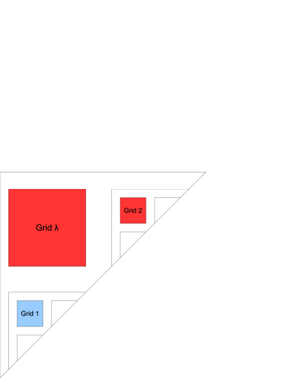
Figure 3: The sequence of subgrids

The next step, which we briefly state, is to define a grid-coloring $\chi_{2}$ with $r^{4}$ colors corresponding to each of the four grids $G_{11},G_{12},G_{21},G_{22}$. We find a subgrid of color $(c_{11},c_{12},c_{21},c_{22})$ under this coloring, which corresponds to four grids, which further restrict one another.

Continue this for $f(2,r)+1$ steps, so that the final grids are indexed by strings of length $f(2,r)$. The “large” monochromatic grid we find under $\chi_{f(2,r)-1}$ need only be a $2\times 2$ grid, giving $G_{s}$ a single off-diagonal point for all $s$ of length $f(2,r)$. The color of this point is $c_{s}$.

We now recognize the map $s\mapsto c_{s}$ as an $r$-coloring of the perfect binary tree of height $f(2,r)$. By the definition of $f$, this coloring must be 1-balanced, meaning there is a node $\sigma$ and two children $s=\sigma\cdot 1\cdot u$ and $t=\sigma\cdot 2\cdot v$, all the same color, where $u,v\in\{1,2\}^{\ell}$ for some $\ell$. Call this color red.

Write $\sigma=\sigma_{0}\sigma_{1}\ldots\sigma_{k-1}$. Since $\sigma$ is red, the monochromatic grid found in grid $G_{\sigma_{k}}$ is red. Let

$$z_{i}(\sigma)=\left\{\begin{array}[]{ll}x_{i}&\hbox{if }\sigma_{i}=1\\ y_{i}&\hbox{if }\sigma_{i}=2.\\ \end{array}\right.$$

Then the grid $G_{\sigma}$ is in position $(X(\sigma),Y(\sigma))$, where

$$\begin{array}[]{rcl}X(\sigma)&=&z_{0}(\sigma)+d_{0}(z_{1}(\sigma)+d_{1}(\ldots(z_{k-1}(\sigma)+d_{k-1}x_{k})\ldots)),\\ Y(\sigma)&=&z_{0}(\sigma)+d_{0}(z_{1}(\sigma)+d_{1}(\ldots(z_{k-1}(\sigma)+d_{k-1}y_{k})\ldots)).\\ \end{array}$$

and has scale $D=d_{0}d_{1}\cdots d_{k}$. Note that the only difference between $X$ and $Y$ is the $x_{k}$ and $y_{k}$ respectively in the inner-most term.

Now we look at the grids $G_{s}$ and $G_{t}$. We will only use a single point from these grids. Define $z_{i},X$, and $Y$ in the same way as above for $s$ and $t$. Noting that

$$s_{0}=\sigma_{0},s_{1}=\sigma_{1},\ldots,s_{k-1}=\sigma_{k-1},s_{k}=1\hbox{ and}$$

$$t_{0}=\sigma_{0},t_{1}=\sigma_{1},\ldots,t_{k-1}=\sigma_{k-1},t_{k}=2,$$

we see that $G_{s}$ is in position $(X(s),Y(s))$ with

$$\begin{array}[]{rcl}X(s)&=&X(\sigma)+D(x_{k}+d_{k}(\ldots(z_{k+\ell-1}(s)+d_{k+\ell-1}x_{k+\ell})\ldots),\\ Y(s)&=&X(\sigma)+D(x_{k}+d_{k}(\ldots(z_{k+\ell-1}(s)+d_{k+\ell-1}y_{k+\ell})\ldots),\\ \end{array}$$

and similarly $G_{t}$ is in position $(X(t),Y(t))$ with

$$\begin{array}[]{rcl}X(t)&=&Y(\sigma)+D(y_{k}+d_{k}(\ldots(z_{k+\ell-1}(t)+d_{k+\ell-1}x_{k+\ell})\ldots),\\ Y(t)&=&Y(\sigma)+D(y_{k}+d_{k}(\ldots(z_{k+\ell-1}(t)+d_{k+\ell-1}y_{k+\ell})\ldots).\\ \end{array}$$

We claim that $X(s),X(t),Y(s),Y(t)$ form our Hilbert cube. Indeed, writing $a=X(s)$, $b=X(t)-X(s)=Y(t)-Y(s)$, and

$$c=Dd_{k}\cdots d_{k+\ell}(y_{k+\ell+1}-x_{k+\ell+1}),$$

we see that they have the form $a,a+b,a+c,a+b+c$ respectively.

Now consider the colors of the six points among these values (still only looking at points above the line $x=y$). Since the points $(X(s),Y(s))$ and $(X(t),Y(t))$ are in $G_{s}$ and $G_{t}$ respectively, we know that both points are red.

Now we recognize that these values are given by

$$\begin{array}[]{rcl}X(s)&=&X(\sigma)+iD,\\ Y(s)&=&X(\sigma)+jD,\\ X(t)&=&Y(\sigma)+iD,\\ Y(t)&=&Y(\sigma)+jD,\\ \end{array}$$

so the four points we need look like

$$\begin{array}[]{rcl}(X(s),X(t))&=&(X(\sigma)+iD,Y(\sigma)+iD)\\ (X(s),Y(t))&=&(X(\sigma)+iD,Y(\sigma)+jD)\\ (Y(s),X(t))&=&(X(\sigma)+jD,Y(\sigma)+iD)\\ (Y(s),Y(t))&=&(X(\sigma)+jD,Y(\sigma)+jD).\\ \end{array}$$

By design, these fall into the grid $G_{\sigma}$, so these points are red as well. ∎

5.2 Upper bounds

The process repeats to a depth of $f(2,r)$, at which point we have $2^{f(2,r)}$ grids, meaning $r^{2^{f(2,r)}}$ colors. At this level, we are looking for a square, so these grids must have size

$$S_{f(2,r)}=2.$$

At the prior level, our $2^{f(2,r)-1}$ grids must have monochromatic subgrids of size $S_{f(2,r)}$, and the joint coloring has $r^{2^{f(2,r)-1}}$ colors. Thus

$$S_{f(2,r)-1}=2GW(S_{f(2,r)},r^{2^{f(2,r)-1}}),$$

where the factor of 2 allows us to take the top-left quadrant of the grid. As before, this ensures distinct values in the $x$ and $y$ components. Repeating this reasoning, we find that

$$S_{k}=2GW(S_{k+1},r^{2^{k}}),$$

which leaves us with this bound for the size of the initial grid:

$$n(r,2)\leq S_{0}=2GW(S_{1},r).$$

5.3 Any colors, any dimensions

We have now done all of the hard work. In order to prove the full result at this point, we only need to reconsider the proof for $k=2$.

Theorem 3.1  For all $r,k$, there is a number $n=n(r,k)$ so that for any $r$-coloring of the edges of the complete graph on $[n]$, there is a Hilbert cube $H=H(a;b_{1},\ldots,b_{k})$ so that all edges within $H$ are monochromatic.

Proof.

Let $\chi$ be an $r$-coloring of a large grid. Repeat the process from the proof in Section 5.1, now continuing until we have a tree of height $E(2,r,k-1)$.

By Lemma 4.4, there is an embedded tree of height $k-1$ which is entirely, say, red. Call the embedding $\varphi$, so the nodes are labeled $\varphi(s)$ for $s\in\{1,2\}^{j}$ for $0\leq j<k$.

Let $G_{s}$ denote the red grid corresponding to the node $\varphi(s)$. Say this grid is in position $(X(s),Y(s))$. If $i$ is the length of $s$, then the scale of $G_{s}$ is $d_{0}d_{1}\cdots d_{i}$.

For each $s\in\{1,2\}^{k-1}$, consider the red point $(X(s),Y(s))\in G_{s}$. We claim that the $2^{k}$ values

$$\{X(s)\mid s\in\{1,2\}^{k-1}\}\cup\{Y(s)\mid s\in\{1,2\}^{k-1}\}$$

have the form $a+\sum_{i\in I}b_{i}$ and comprise an entirely red clique.

As we saw in the previous proof, for $s$ on level $\ell-1$, and $s\cdot 1,s\cdot 2$ on level $\ell$,

$$X(s\cdot 2)-X(s\cdot 1)=Y(s)-X(s)=d_{0}d_{1}\cdots d_{\ell-1}(y_{\ell}-x_{\ell}).$$

Inspired by this, we define

$$b_{\ell}=Y(s)-X(s)$$

for $s$ on level $\ell-1$.

Now set $a=X(1^{k-1})$. Let $s=s_{1}\cdots s_{k-1}\in\{1,2\}^{k-1}$. Let $I=\{i\mid s_{i}=2\}\subseteq[k-1]$. This gives us $X(s)=a+\sum_{i\in I}b_{i}$ and $Y(s)=a+b_{k}+\sum_{i\in I}b_{i}$.

This tells us the numbers we are looking at really do have the desired form. We only need to check that all the edges among these values are red.

Let $s$ be any string on level $k-1$. By virtue of $(X(s),Y(s))$ being a point in the grid $G_{s}$, we know that edge is red. Now let $t$ be another string on level $k-1$, and assume $s<t$ lexicographically. Let $\sigma$ be the longest initial string that $s$ and $t$ agree on — their closest common ancestor. Since $s<t$, we must have that $s=\sigma\cdot 1\cdot u$ and $t=\sigma\cdot 2\cdot v$ for some $u$ and $v$ of the same length.

As we saw in the previous proof, since $G_{\sigma}$ is red, we immediately get that $(X(s),X(t)),(X(s),Y(t)),(Y(s),X(t)),(Y(s),Y(t))$ are all red.

By considering all possible $s,t$ on level $k-1$, this argument says that all edges among these values are red, so we have reached our goal. ∎

Along the same lines as Section 5.2, we may define the recurrence

$$T_{E(2,r,k)}=2,\hbox{ and}$$

$$T_{k}=2GW(T_{k+1},r^{2^{k}}),$$

to get an upper bound of

$$n(r,k)\leq T_{0}=2GW(T_{1},r).$$

5.4 Additional results

Theorem 3.1 immediately gives several nice consequences.

By considering subsets of Hilbert cubes, it is easy to see that, for large $n$, any edge-coloring of the complete graph on $[n]$ will always have solutions to equations of the form $x_{1}+\ldots+x_{\ell}=y_{1}+\ldots+y_{\ell}$ which induce monochromatic subgraphs.

Combining Theorem 3.1 with Szemerédi’s celebrated theorem on arithmetic progressions [10], we get the following nice corollary.

Corollary 5.1.

For any $\delta>0$, and naturals $r,k$, there is a number $n=n(r,\delta)$ so that for any set $A\subseteq\mathbb{N}$ of upper density $\delta$, and any $r$-coloring of the edges of the complete graph on $A$, there is a Hilbert cube $H=H(a;d_{1},\ldots,d_{k})$ contained in $A$ so that all edges within $H$ are monochromatic.

On the other hand, our theorem also inspires another negative result. A Hilbert cube of dimension 2 is simply a set satisfying $w-x=y-z$. We consider a similar equation, $a(w-x)=b(y-z)$, for $a\neq b$ fixed. To avoid this equation, color pairs based on their difference. Write $|w-x|=\left(\frac{b}{a}\right)^{k}p$ for $k$ as large as possible, and color $\{w,x\}$ by the parity of $k$. Since $(w-x)$ and $(y-z)$ will always be different by a factor of $\frac{b}{a}$, this will assure the edges $\{w,x\}$ and $\{y,z\}$ have different colors.

6 Acknowledgment

The author would like to thank Ron Graham for his guidance, which helped to strengthen the main theorem.

References

- [1] W. Deuber, D. S. Gunderson, N. Hindman, D. Strauss, Independent finite sums for -free graphs, J. Combin. Theory Ser. A 78 (1997), no. 2, 171-198.
- [2] R.L. Graham, B.L. Rothschild, Ramsey’s Theorem for -Parameter Sets, Trans. Amer. Math. Soc. 159 (1971), 257-292.
- [3] R.L. Graham, B.L. Rothschild, J. Spencer, Ramsey Theory, John Wiley & Sons Inc., New York, second edition 1990.
- [4] D. S. Gunderson, I. Leader, H. J. Prömel, and V. Rödl, Independent arithmetic progressions in clique-free graphs on the natural numbers, J. Combin. Th. Ser. A 93 (2001), 1-17.
- [5] D. Hilbert, Über die Irreduzibilität ganzer rationaler Funktionen mit Ganzzahligen Koeffizienten, J. Reine Angew. Math. 110 (1892), 104-129.
- [6] A. V. Kostochka, M. Stiebitz, B. Wirth, The colour theorems of Brooks and Gallai extended, Discrete Mathematics, Volume 162, Issues 1-3, 25 December 1996, 299-303.
- [7] R. Rado, Studien zur Kombinatorik, Math. Zeit. 36 (1933), 242-280.
- [8] F. P. Ramsey, On a problem in formal logic, Proc. London Math. Soc. (2), 30 (1930), 264-286.
- [9] I. Schur, Über die Kongruenz , Jber. Deutsch. Math. Verein 25 (1916), 114-116.
- [10] E. Szemerédi, On sets of integers containing no elements in arithmetic progression, Acta Arithmetica 27 (1975), 199-245.
- [11] B. L. van der Waerden, Beweis einer Baudetschen Vermutung, Nieuw Arch. Wiskunde 15 (1927), 212-216.
- [12] E. Witt, Ein kombinatorischer Satz der Elementargeometrie, Math. Nachrichten 6 (1952), 261-262.