Implementing quantum gates by optimal control with doubly exponential convergence

Abstract

We introduce a novel algorithm for the task of coherently controlling a quantum mechanical system to implement any chosen unitary dynamics. It performs faster than existing state of the art methods by one to three orders of magnitude (depending on which one we compare to), particularly for quantum information processing purposes. This substantially enhances the ability to both study the control capabilities of physical systems within their coherence times, and constrain solutions for control tasks to lie within experimentally feasible regions. Natural extensions of the algorithm are also discussed.

The coherent control of quantum mechanical systems wiseman_quantum_2009 ; shapiro_principles_2003 has been sucessfully applied to a growing number of tasks in recent years dowling_quantum_2003 ; mabuchi_principles_2005 . The early approaches such as two pathway quantum interference, pump-dump schemes, or stimulated Raman adiabatic passage are intrinsically understandable in terms of interference due to the coordinated activation of resonant transitions between few energy levels brif_control_2010 . In order to extend such strategies and tackle more challenging problems, the field has moved towards employing pulse shapers and optimization algorithms singer_colloquium:_2010 .

The field has also broadened its scope, from problems of state preparation, or more generally maximizing the value of an observable over an ensemble tannor_control_1985 , to, in particular, implementing unitary maps schulte-herbrueggen_optimal_2005 . This latter bridges the gap between physical dynamics and the gate formalism of quantum information processing, for which high accuracy solutions are sought, ultimately aiming to reach an error correction threshold around $10^{-3}$ to $10^{-4}$ per gate or below steane_overhead_2003 . In applying the same methods to both state, and map or gate problems, the additional structure inherent to gate problems has however been neglected – the aim of this letter is to describe how this structure can be exploited to better understand and substantially ease the solving of gate problems.

Formally, a closed $N$-level system undergoes controlled unitary dynamics given by $U_{\text{{{f}}}}$ satisfying

$$\frac{\partial}{\partial t}U_{\text{{{f}}}}(t)=-iH[\text{{{f}}}(t)]U_{\text{{{f}}}}(t),\quad U_{\text{{{f}}}}(0)=I$$

with $I$ the identity matrix, and a time dependent Hamiltonian

$$H[\text{{{f}}}(t)]=H_{0}+\sum_{r=1}^{R}\text{{{f}}}_{r}(t)H_{r}$$ (1)

where f is a set of $R$ controls pulses, altering the system potential within a semi-classical model under the bilinear approximation. The abstract control problem for a target unitary gate $V$ consists in finding a set of real valued functions f and an evolution time $T$ such that the dynamics satisfies $U_{\text{{{f}}}}(T)=V$. Since this entails transferring a full basis of states to another (with relative phases), the intuition applicable to state problems is no longer available, and in fact schemes to solve it explicitly are limited to two level systems, or special cases with few levels. For practical purposes, we would only require the actual $U_{\text{{{f}}}}(T)$ and target $V$ to match up to some prescribed error level $\varepsilon$, with respect to a notion of distance $d$. Optimisation, whereby a sequence of pulses $\text{{{f}}}^{(n)}$ is generated iteratively with the requisite distance $d(U_{\text{{{f}}}^{(n)}}(T),V)$ decreasing at each step, has emerged as the strategy of choice for achieving this. The definitions of distance $d(U,V)$ to measure the error have generally been based on the Hilbert-Schmidt norm, using either $\|U-V\|$ or, quotienting out the unphysical global phase of the dynamics and normalising,

$$d(U,V)=\frac{1}{2\sqrt{N}}\min_{\varphi}\|U-e^{i\varphi}V\|$$

which we will be using herein. In contrast to state control problems where intuitive understanding often plays a role in choosing the initial trail pulses $\text{{{f}}}^{(0)}$, the serious limitations of intuitive insight for gate problems lead to $\text{{{f}}}^{(0)}$ typically being chosen arbitrarily, eg. at random. Moreover, to get any measure of gate error based on experimental measurement would require exhaustive and arduous process tomography, so that there has been an overwhelming preference towards working with numerical simulation of a model for the system.

Running a numerical optimisation algorithm requires that the control pulses be discretised, and in order to incorporate experimental constraints we can choose a basis for discretisation corresponding to the capabilities of our pulse shaping equipment. Thus we let

$$\text{{{f}}}_{r}(t)=\sum_{k=1}^{K}\alpha_{rk}b_{k}(t)$$

and then optimise over the set of $RK$ coefficients $\alpha_{rk}$; ideally the basis elements $b_{k}$ would be precisely calibrated to the equipment, but for definiteness we will consider representatives of two important cases. A common choice in the literature, and the main one we will use, is that of piecewise constant functions, as can be produced by an arbitrary waveform generator motzoi_optimal_2011 . In the case of frequency domain pulse shaping, we are dealing with functions which, up to Gaussian tails, are both time and spectral bandwidth limited. To capture this property, under suitable scaling we can let $b_{k+1}$ be the Hermite function of index $k$, and restrict to the first $K$ of these. Such a choice has on the other hand not been used in the quantum control setting to our knowledge, although the benefits of Hermite functions have certainly been exploited in other applications, eg. higuchi_multiplex_1968 – while the smoother alternatives to piecewise constant functions used, such as truncated interpolating polynomials li_optimal_2011 , have much fatter tails in frequency domain. In addition to the basis constraint on the pulses f, there must clearly be some bound $B$ on the pulse fluences, equivalently their magnitude in the integrated power norm.

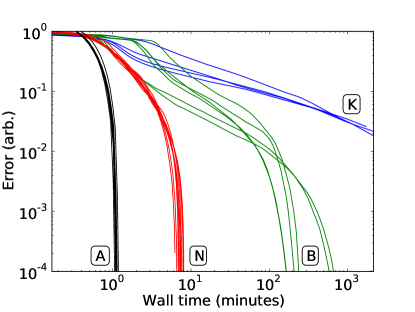
Figure 1: Performance comparison between several runs of the Newton-Raphson (red, labeled ‘N’), BFGS GRAPE (green, labeled ‘B’) and Krotov (blue, labeled ‘K’) algorithms with small initial pulses $\text{{{f}}}^{(0)}$. Also shown (in black, labeled ‘A’) are Newton-Raphson runs initialised at the norm with least ill-conditioning; the cost of finding this norm, on average 21 seconds, is included.

For generic intrinsic and control Hamiltonians $H_{0},\ldots,H_{R}$ of (1), as well as many specific cases of physical interest, full controllability is known to hold, meaning that any target gate can be achieved given sufficient evolution time $T$ and freedom in shaping the control pulses jurdjevic_control_1972a . While this is a strong result, it does not identify which gates are achievable for particular evolution times and constraints on the controls, in any given experimental context. Indeed, such specific results are currently lacking, and one must resort to numerical investigations in order to gain better understanding into the capabilities of each physical system caneva_optimal_2009 . This motivates the need for an optimisation algorithm to solve the gate problem in runtimes on a scale rendering the process interactive or faster. It is the purpose of this letter to introduce a Newton-Raphson root finding approach for this problem, which performs substantially faster than existing methods (see Fig. 1), thereby achieving this goal on non-trivial examples. Such an approach also sheds light on the strong influence of the pulse initialisation $\text{{{f}}}^{(0)}$, leading to a prescription for how to choose it.

For consistency, all numerical examples herein are for the canonical problem of implementing a quantum Fourier transform on a five qubit Ising coupled spin chain in a magnetic field gradient using two controls. But these are qualitatively representative of the results for different evolution times, target gates, and modes of control – a different problem scenario illustrates such similarity in the supplement. In terms of Pauli matrices $\sigma$, the Hamiltonian in question is

$$H\left[\text{{{f}}}\left(t\right)\right]=\sum_{n=1}^{4}\sigma_{z}^{\left(n\right)}\sigma_{z}^{\left(n+1\right)}-\sum_{n=1}^{5}\left(n+2\right)\sigma_{z}^{\left(n\right)}\\ +\text{{{f}}}_{1}\left(t\right)\sum_{n=1}^{5}\sigma_{x}^{\left(n\right)}+\text{{{f}}}_{2}\left(t\right)\sum_{n=1}^{5}\sigma_{y}^{\left(n\right)}$$ (2)

while we fix an evolution time $T$ of $125$ and use $K=1000$ basis functions, with piecewise constant controls unless stated otherwise.

Over the last fifteen years, most techniques successfully applied to model-based quantum control problems have either come from mainstream gradient-driven optimisation theory, eg. conjugate gradient and BFGS de_fouquieres_second_2011 based GRAPE khaneja_optimal_2005 algorithms, or can be understood in this context, as with the Krotov method maday_new_2003 . These state of the art techniques have led to advances such as towards implementing logic gates fault-tolerantly nigmatullin_implementation_2009 or with minimal errors given the decoherence time spoerl_optimal_2007 . They owe their performance to the use of gradient information, but a key realisation is that the full Jacobian matrix $\tilde{J}$ of $U_{\text{{{f}}}}(T)$ for the gate problem can be computed as efficiently as its single row constituting the gradient vector. Indeed the usual gradient computation kuprov_derivatives_2009 , for $\|U_{\text{{{f}}}}(T)-V\|^{2}$ say, effectively proceeds through $\tilde{J}$ by inner producting each row of $\tilde{J}$ with $V$, so that using the gradient alone means discarding a lot of valuable information.

Looking at the singular value decomposition of the Jacobian matrix leads to a clean geometric picture, whereby changes to the pulses below a certain norm $r$ (beyond which higher order terms cease being negligible) induce changes in the implemented gate within a prescribed ellipsoid. The basic Newton-Raphson iteration kelley_solving_2003 then consists in using this Jacobian model, with a heuristic choice of $r$, to compute new pulses bringing the implemented $U(T)$ closer to the target $V$, which reduces to a linear algebraic task. In order to have the modelling ellipsoid strictly track the unitary group, one can map its elements down via the matrix exponential, or conversely, group elements up via the matrix logarithm, as we describe later. The volume of this ellipsoid determines the ability of all algorithms mentioned herein to shift $U_{\text{{{f}}}}(T)$ in general directions, while for the specific target $V$ a more relevant quantity correlated to this volume is the distance to exact solution controls upon ignoring higher order terms, which we shall refer to as the level of ill-conditioning.

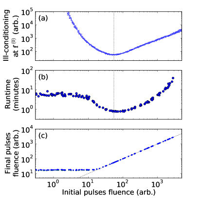
Figure 2: For Newton-Raphson runs with initial pulses $\text{{{f}}}^{(0)}$ of different norms, (b) the wall time needed to reach an error $\varepsilon$ of $10^{-4}$ and (c) the norm of the corresponding solution pulses, with a dashed ‘initial equals final’ line. In addition, (a) the ill-conditioning of the Jacobian at several randomly sampled pulses of each norm.

The situation for our test problem depicted in Fig. 2 is representative of the general structure, as described in detail in the supplemental material, which can be expected of all problems. We see that both the ill-conditioning and the Newton-Raphson runtime strongly depend on the integrated power of the pulses (specifically of $\text{{{f}}}^{(0)}$ in the latter case), but are well concentrated beyond this along a single curve, with the minimum of these two curves coinciding. When solution pulses are required to have a fluence below $B$, we can cheaply find the minimum of the ill-conditioning curve restricted to the interval $\left[0,4B/5\right]$ say, and use an arbitrary $\text{{{f}}}^{(0)}$ with this norm to initialise the algorithm. It is clear from Fig. 2(c) that this choice will yield a solution satisfying the fluence constraint unless no choice can, while the correspondance between ill-conditioning and runtime curves makes it the most efficient choice. The benefit of this prescription over less deliberate ones is evident from comparing the ‘A’ and ‘N’ series of runs in Fig. 1.

The original equation $U_{\text{{{f}}}}(T)=V$ should be thought of as over-determined when the dimension $N^{2}$ of the unitary group is greater than that of the control space $RK$, since then it is only solvable to arbitrarily high accuracy for an exceptional set of targets $V$. This makes it an unfavourable case in the context of low error control, because it is implausible for a target gate $V$ of interest to be special in this sense. On the other hand, whenever solvability is not so limited then almost every achievable target $V$ admits an $RK-N^{2}$ dimensional set of control pulses implementing it. Although the number of iterations for algorithms to reach a given error tolerance $\varepsilon$ is, as expected, reduced as this dimension of degeneracy increases, there is a counter-intuitive downside to under-determined problems.

In general when converging to an exact solution, the error of Krotov iterates decays exponentially, ie. eventually as $\gamma^{n}$ for some $\gamma<1$, while with conjugate gradient or BFGS, the error decay is faster than exponential, and Newton algorithms have error decaying doubly exponentially ben-israel_newton-raphson_1966 , as $O(\beta^{2^{n}})$ for some $\beta$. But in the under-determined context, one can only count on exponential convergence from all of these algorithms except for Newton-Raphson root finding which retains its double exponential convergence. Indeed, the directions of degeneracy about a solution form a null space to the Hessian there, rendering inapplicable the analysis dennis_characterization_1974 on which faster than exponential convergence results for BFGS are based powell_global_1976 ; li_global_2001 . The stark difference between these rates is illustrated in Fig. 3, where all Newton-Raphson runs surpass $10^{-4}$ in a single iteration once they reach $10^{-2}$ error.

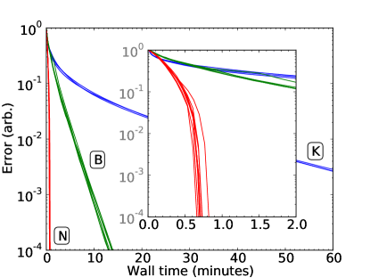
Figure 3: Illustration of the different convergence behaviours of Newton-Raphson (red, labeled ‘N’), BFGS GRAPE (green, labeled ‘B’) and Krotov (blue, labeled ‘K’) algorithms with initial norms having minimal ill-conditioning. Although several runs were carried out from very different initial pulses, the performance profile of each algorithm remains the same.

In order to make best use of Newton-Raphson root finding, we must re-formulate our problem over a linear space, and the most natural choice here is to seek for the functional

$$\mathfrak{L}(\text{{{f}}})=\log\left(V^{{\dagger}}U_{\text{{{f}}}}(T)\right)$$

to equal zero within the space $\mathfrak{u}$ of anti-Hermitian matrices. The resulting algorithm then has the elegant property of reducing the geodesic distance between the actual $U_{\text{{{f}}}}(T)$ and target gate $V$ on each iteration. It can usefully be made more general by restricting attention to a subspace of $\mathfrak{u}$, specified by an orthogonal projection $P$, ie. seeking a zero of $P\mathfrak{L}(\text{{{f}}})$. In particular, restricting to the space $\mathfrak{s}\mathfrak{u}$ of traceless anti-Hermitian matrices makes the root finding insensitive to the unphysical global phase.

A less obvious application is to implement a gate on a system interacting coherently with an environment rebentrost_optimal_2009 , which contrary to Markovian interaction with a bath is reversible so need not fundamentally limit the achievable error. The full Hilbert space then splits as $S\otimes E$, and for a given gate on the system $W$ our aim would be to implement any gate of the form $W\otimes A$ for an ancillary evolution $A$ – this corresponds to letting $V=W\otimes I$ in $\mathfrak{L}$ and projecting it out of the space $I\otimes\mathfrak{u}$ with $P$. Although the Newton-Raphson algorithm can certainly be applied to Lindblad dynamics, choosing a short evolution time $T$ to limit dissipation and finding a control for the system without bath should still be a first step, since computing the evolution super-operator is much more expensive. In both extensions, having $RK\geqslant N^{2}$ becomes far from sufficient to justify concluding the problem is exactly solvable.

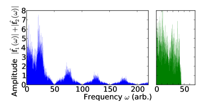
Figure 4: Spectrum of typical minimal norm solutions with error below $10^{-4}$, in the piecewise constant (left) and Hermite function (right) bases. These are symmetric about $\omega=0$, but the Hermite functions could just as easily be made bandlimited about any chosen carrier frequency.

Up until now, all numerical examples have been in the piecewise constant basis, but our algorithm applies to general bases, and of particular interest is the Hermite basis to find spectrally narrow solution pulses. Note that the same bandwidth as seen in the right panel of Fig. 4 could be obtained by a suitable basis of low frequency Fourier components, but implementing such a pulse in a finite time duration would lead to distortion, thereby deteriorating the achieved error. Interestingly, using the same number of basis functions $K$, the curve from Fig. 2(c) and the most efficient initial fluence remain unchanged across both bases – the average number of iterations to reach the same error tolerance $\varepsilon$ is also similar (10.1 vs. 12.5) for this initial fluence. The piecewise constant basis is however special in how operations are cheaper with it than in general bases, eg. for our test problem computing the propagator $U_{\text{{{f}}}}\left(T\right)$ takes 0.9 seconds, as opposed to around 50 seconds in the Hermite basis. This makes it all the more important to choose the initial $\text{{{f}}}^{(0)}$ in a general basis carefully, and to this end information from the more tractable piecewise constant case seems to suffice.

We have seen how viewing unitary map control problems from the root finding perspective motivates an algorithm offering vast performance improvements over existing methods, and reveals particularly clean structure within the space of controls. This formulation can moreover naturally be made in the full generality of pulses represented in arbitrary bases and accounting for an environment to the system. For state preparation problems, considering the Newton-Raphson algorithm analogue martinez_quasi-newton_1991 in that case promises to lead to further fruitful developments.

This work was funded by EPSRC, via CASE/CNA/07/47, and Hitachi. The author wishes to thank Sophie Schirmer and Peter Pemberton-Ross for valuable exchanges.

I Supplemental material

We will now describe the algorithm as implemented for producing numerical results in this work, aiming to include sufficient technical detail that it may be fully replicated based on this account. This specification focuses on the resulting performance more than ease of implementation, and most of its prescriptions can be legitimately simplified as needed. A source code release, to be made available as a Python SciKit under the code-name CUMIN, is also in preparation.

I.1 Numerical optimisation

A common thread in derivative-based optimisation nocedal_numerical_1999 , aiming to minimise an objective function $\mathfrak{E}:\mathbbm{R}^{M}\rightarrow\mathbbm{R}$, is the repeated update of a variable $\boldsymbol{a}$ storing what can be thought of as the current base point for the domain $\mathbbm{R}^{M}$. We will write $\boldsymbol{a}^{\left(0\right)},\boldsymbol{a}^{\left(1\right)},\ldots$ for the sequence of values taken by $\boldsymbol{a}$, but omit the superscript when referring to its value at some present state of the algorithm. On each iteration, say the $n^{\operatorname{th}}$, a model for $\mathfrak{E}$ valid locally about the outgoing base point $\boldsymbol{a}^{\left(n-1\right)}$ for this iteration is constructed based on the value of certain derivatives of function $\mathfrak{E}$ at the point $\boldsymbol{a}^{\left(n-1\right)}$. The idea is then to take for the next base point $\boldsymbol{a}^{\left(n\right)}$ the minimum $\boldsymbol{v}$ of this model for $\mathfrak{E}$, possibly restricted to some neighbourhood of $\boldsymbol{a}^{\left(n-1\right)}$. However, since the model is only valid locally, we cannot guarantee $\mathfrak{E}\left(\boldsymbol{v}\right)<\mathfrak{E}(\boldsymbol{a}^{\left(n-1\right)})$ ie. that using $\boldsymbol{v}$ as the next base point will lead to a reduction of the current objective value $\mathfrak{E}\left(\boldsymbol{a}\right)$. Two families of approaches exist for resolving this problem: line search methods look for a suitable point along the line starting at $\boldsymbol{a}^{\left(n-1\right)}$ in the direction of $\boldsymbol{v}$, while trust region methods consider rescaling the neighbourhood of $\boldsymbol{a}^{\left(n-1\right)}$ to which they constrain minimisation of the model for $\mathfrak{E}$.

The main performance characteristic which can be reliably affected in choosing between derivative-based optimisation algorithms is the run-time required to achieve convergence to a given accuracy. When methods have different asymptotic rates of convergence, one of them is determined in advance to eventually be closer to the limit than all others. Prior to this regime, there is a trade-off in the accuracy of models used on each iteration, where more derivative information can be acquired at higher computational cost to construct better models, which should in contrast enable greater progress per iteration. In this respect, the Hessian matrix of all $M\left(M+1\right)/2$ second derivatives is prohibitively expensive to compute except for special $\mathfrak{E}$, so that widely effective algorithms only require the gradient vector of $M$ first derivatives.

For example quasi-Newton optimisation methods, of which BFGS is an instance, use the model $\mathfrak{E}\left(\boldsymbol{a}+\boldsymbol{p}\right)\simeq\mathfrak{E}\left(\boldsymbol{a}\right)+\boldsymbol{g}^{\mathrm{T}}\boldsymbol{p}+\frac{1}{2}\boldsymbol{p}^{\mathrm{T}}B\boldsymbol{p}$ where $\boldsymbol{g}$ is the gradient vector of $\mathfrak{E}$ at $\boldsymbol{a}$, and $B$ is constructed iteratively to approximate the Hessian matrix of $\mathfrak{E}$ at $\boldsymbol{a}$. At least for BFGS, the model minimum $\boldsymbol{v}$, namely $-B^{-1}\boldsymbol{g}$ since $B$ is always positive definite, is used within a line search routine at each iteration. In this context, steepest descent would correspond to replacing $B$ by the identity matrix $I$, but we do not consider this method since it cannot be recommended in general, and performs particularly slowly on gate control problems machnes_comparing_2011 . For comparison, convergence of BFGS iterates to a local minimum $\boldsymbol{a}^{\ast}$ where the Hessian of $\mathfrak{E}$ is positive definite is understood to happen at a rate, measured either by $\|\boldsymbol{a}^{\left(n\right)}-\boldsymbol{a}^{\ast}\|$ or $\mathfrak{E}(\boldsymbol{a}^{\left(n\right)})-\mathfrak{E}\left(\boldsymbol{a}^{\ast}\right)$, between $O(\xi^{n\log n})$ griewank_global_1991 and $\Omega(\xi^{n^{2}})$ powell_rate_1983 for some problem specific $\xi$. While convergence for conjugate gradient powell_convergence_1976 and limited memory BFGS liu_limited_1989 , without being restarted every $M$ iterations only goes as $\xi^{n}$ asymptotically, which is also the rate for steepest descent albeit with $\xi$ deteriorating significantly akaike_successive_1959 on poorly conditioned problems.

I.2 Newton-Raphson method

This description can be adapted to cover Newton-Raphson root finding applied to the vector valued function $\mathfrak{L}:\mathbbm{R}^{M}\rightarrow\mathbbm{R}^{m}$ by introducing an objective function $\mathfrak{E}\left(\boldsymbol{x}\right)=\|\mathfrak{L}\left(\boldsymbol{x}\right)\|^{2}$ and specifying that the model, hence the derivatives used to construct it, should be of $\mathfrak{L}$ rather than $\mathfrak{E}$. The model in this case reads

$$\mathfrak{L}\left(\boldsymbol{a}+\boldsymbol{p}\right)\simeq\mathfrak{L}\left(\boldsymbol{a}\right)+J\boldsymbol{p}$$

where $J$ is the Jacobian matrix of $\mathfrak{L}$ at the point $\boldsymbol{a}$, with entry $i,j$ equal to the $j^{\operatorname{th}}$ partial derivative $\frac{\partial}{\partial x_{j}}$ of the $i^{\operatorname{th}}$ component of $\mathfrak{L}\left(\boldsymbol{x}\right)$ – in the notation of differential geometry, we can succinctly write $J$ as $\mathrm{d}\mathfrak{L}|_{\boldsymbol{a}}$.

If the model were exact, assuming the rank of $J$ equals $m$, a global minimum of $\mathfrak{E}$ could be found where $\mathfrak{L}$ is $\boldsymbol{0}$, namely at $\boldsymbol{a}+\boldsymbol{p}$ with $\boldsymbol{p}$ being any solution to $J\boldsymbol{p}=-\mathfrak{L}\left(\boldsymbol{a}\right)$. Indeed the classical Newton-Raphson algorithm, applicable for dimensions $M=m$, uses the update rule $\boldsymbol{a}^{\left(n+1\right)}=\boldsymbol{a}^{\left(n\right)}+\boldsymbol{p}$ for which $\mathfrak{E}(\boldsymbol{a}^{\left(n\right)})$ goes to zero doubly exponentially in $n$, specifically as $O(\beta^{2^{n}})$ for some $\beta$ (known as quadratic convergence), for suitable initial conditions $\boldsymbol{a}^{\left(0\right)}$. Generalising this to the under-determined regime $M>m$, the value of $\boldsymbol{p}$ is no longer explicitly determined as $-J^{-1}\mathfrak{L}\left(\boldsymbol{a}\right)$, and a suitable choice for $\boldsymbol{p}$ which preserves the quadratic convergence property is the minimum norm solution of $J\boldsymbol{p}=-\mathfrak{L}\left(\boldsymbol{a}\right)$ ben-israel_newton-raphson_1966_sup , computable as $-J^{\mathrm{T}}(JJ^{\mathrm{T}})^{-1}\mathfrak{L}\left(\boldsymbol{a}\right)$. In either case, a suitable initial $\boldsymbol{a}^{\left(0\right)}$ would be any point sufficiently close to some solution $\boldsymbol{a}^{\ast}$ of $\mathfrak{L}\left(\boldsymbol{a}^{\ast}\right)=\boldsymbol{0}$ where the Jacobian $\mathrm{d}\mathfrak{L}|_{\boldsymbol{a}^{\ast}}$ has full rank $m$, in such a way that $\mathrm{d}\mathfrak{L}|_{\boldsymbol{a}^{\left(n\right)}}$ is always full rank so that all iterates $\boldsymbol{a}^{\left(n\right)}$ are well-defined.

Finding such an initial point is itself difficult, and for general points $\boldsymbol{a}$ the neighbourhood in which the model at $\boldsymbol{a}$ is accurate contains neither a root $\boldsymbol{a}^{\ast}$ of $\mathfrak{L}$, nor a root $\boldsymbol{a}+\boldsymbol{p}$ of the model. The rationale behind the update rule $\boldsymbol{a}^{\left(n+1\right)}=\boldsymbol{a}^{\left(n\right)}+\boldsymbol{p}$, that $\boldsymbol{a}^{\left(n+1\right)}$ should be close to a root of $\mathfrak{L}$ since $\mathfrak{L}(\boldsymbol{a}^{\left(n\right)}+\boldsymbol{p})\approx\boldsymbol{0}$, therefore no longer applies for general $\boldsymbol{a}^{\left(n\right)}$ and we are compelled to invoke a line search or trust region method to find a usable $\boldsymbol{a}^{\left(n+1\right)}$. But before we delve further into this, let us deal more specifically with the function $\mathfrak{L}$ which we use for the unitary map control problem. Note in passing that for a general objective $\mathfrak{E}$ which is strictly convex at some minimiser $\boldsymbol{a}^{\ast}$, applying Newton-Raphson to its gradient vector $\boldsymbol{g}\left(\boldsymbol{x}\right)=\mathrm{d}\mathfrak{E}|_{\boldsymbol{x}}$ will seek a critical point of $\mathfrak{E}$ so must converge to $\boldsymbol{a}^{\ast}$ when starting sufficiently close to it. The direction of line searches would then be $-J^{-1}\boldsymbol{g}$ where $J$ is the Hessian matrix of $\mathfrak{E}$, justifying the approximating $-B^{-1}\boldsymbol{g}$ used in BFGS.

I.3 Unitary map problem

Consider the dynamical Lie algebra $\mathfrak{l}$ of our control system, ie. the linear space spanned by all iterated commutator expressions starting with the matrices $iH_{0},iH_{1},\ldots,iH_{R}$. By the Frobenius theorem, the propagators $U_{\text{{{f}}}}\left(t\right)$ must remain within the associated group $e^{\mathfrak{l}}$, consisting of matrix exponentials of matrices in $\mathfrak{l}$, for all time and over all possible control vectors $\left(f_{1},\ldots,f_{R}\right)$. Conversely, the controllability theory of bi-linear systems shows that for compact $e^{\mathfrak{l}}$ there is a critical time $T_{c}$ depending only on the system such that every point of $e^{\mathfrak{l}}$ is accessible in some time $T<T_{c}$ using some control vector f. This result also holds if the class of admissible controls is restricted to both smooth or piecewise constant functions. At least when in addition $\mathfrak{l}$ is semi-simple helgason_differential_1981 , the set of unitary matrices $U_{\text{{{f}}}}\left(T\right)$ which are accessible at a fixed time $T$ using some control vector f has non-empty interior within $e^{\mathfrak{l}}$ jurdjevic_control_1972b , for each $T>0$, and in fact equals $e^{\mathfrak{l}}$ for $T$ sufficiently large. The conditions of $e^{\mathfrak{l}}$ being compact and $\mathfrak{l}$ semi-simple will be assumed in what follows – they hold in particular for the Lie algebra of traceless $N\times N$ anti-Hermitian matrices $\mathfrak{s}\mathfrak{u}\left(N\right)$, which is of special interest as it corresponds to full controllability up to global phase.

Once we have introduced a desired parametrisation of the controls, the discretised propagator $U_{\boldsymbol{a}}\left(T\right)$ is a function mapping $\mathbbm{R}^{RK}\rightarrow\text{U}\left(N\right)$, taking a vector $\boldsymbol{a}$ composed of all parameters $\alpha_{rk}$ to the unitary matrix describing the evolution under the corresponding controls. Explicitly, $U_{\boldsymbol{a}}\left(T\right)$ equals the functional $U_{\text{{{f}}}}\left(T\right)$ composed with the synthesis operator taking $\boldsymbol{a}$ to the vector f of functions such that $\text{{{f}}}_{r}(t)=\sum_{k=1}^{K}\alpha_{rk}b_{k}(t)$. Solving $U_{\boldsymbol{a}}\left(T\right)=V$ can naturally be phrased as finding the root of either $U_{\boldsymbol{a}}\left(T\right)-V$ or $V^{{\dagger}}U_{\boldsymbol{a}}\left(T\right)-I$, but both of these functions range over a non-linear space, making them unsuitable for use in the Newton-Raphson algorithm.

Now let $\mathfrak{u}\left(N\right)$ denote the real linear space of all $N\times N$ anti-Hermitian matrices with inner product $\langle A,B\rangle=\operatorname{Tr}\left(A^{{\dagger}}B\right)$. Amongst maps taking the unitary group to a linear space, the inverse $\log:\text{U}\left(N\right)\rightarrow\mathfrak{u}\left(N\right)$ of the well-studied exponential map is a complex analytic function whose value at $I$ is $0$ and derivative there is the identity on $\mathfrak{u}\left(N\right)$ – for $N>2$, it is crucially the only such function taking the global phase neglecting subgroup $\operatorname{SU}\left(N\right)$ to a linear space kang_volume-preserving_1995 . The most natural way to linearise our problem is therefore to look for a root of

$$\mathfrak{L}\left(\boldsymbol{a}\right)=P\log\left(V^{{\dagger}}U_{\boldsymbol{a}}\left(T\right)\right)$$

where the branches of the logarithm are chosen to give a result in $\mathfrak{l}+i\mathbbm{R}I$ of minimal norm and $P$ then expresses this in an orthonormal basis of $\mathfrak{l}$, dropping any $iI$ component. Note that when $\mathfrak{l}$ is $\mathfrak{s}\mathfrak{u}\left(N\right)$, the choice of branches for each eigenvalue is the standard one with imaginary part in $\left(-\pi,\pi\right]$, while the implementation of $P$ can just keep each strictly upper triangular entry of the input matrix and expresses the imaginary part of its diagonal in any orthonormal basis containing the vector of all $1/\sqrt{N}$. This choice for $\mathfrak{L}$ also has the advantage, when $e^{\mathfrak{l}}$ is compact, of making the corresponding error $\sqrt{\mathfrak{E}\left(\boldsymbol{a}\right)}=\|\mathfrak{L}\left(\boldsymbol{a}\right)\|$ equal the geodesic distance between $U_{\boldsymbol{a}}\left(T\right)$ and $V$ over the group $e^{\mathfrak{l}}/\text{U}\left(1\right)$, ie. $e^{\mathfrak{l}}$ quotiented out by global phase (see arvanitogeorgos_introduction_2003 Sect. 3.2).

In its strong form federer_geometric_1996 , Sard’s theorem gives that the set of target gates $V$ in $e^{\mathfrak{l}}/\text{U}\left(1\right)$ for which a solution $\boldsymbol{a}^{\ast}$ to $U_{\boldsymbol{a}^{\ast}}\left(T\right)\equiv V$ exists with rank deficient Jacobian $\mathrm{d}\mathfrak{L}|_{\boldsymbol{a}^{\ast}}$ is of Hausdorff dimension at most $m-1$. Here $m$ is still the dimension of the co-domain of $\mathfrak{L}$, namely $\mathfrak{l}$, which makes $m=N^{2}-1$ in the most prominent case when $\mathfrak{l}$ is $\mathfrak{s}\mathfrak{u}\left(N\right)$. Suppose the $K$, with $M=RK>m$, linearly independent basis functions $b_{k}$ are not so degenerate that the image of $\mathfrak{L}$ is a measure zero set. With respect to choosing a target $V$ from the accessible set, of all $U_{\boldsymbol{a}}\left(T\right)$ for fixed $T$, the full rank condition implying quadratic convergence of the Newton-Raphson algorithm therefore occurs with probability one.

I.4 Computing the Jacobian

The chain rule gives a decomposition for each column

$$\frac{\partial}{\partial\alpha_{rk}}\mathfrak{L}\left(\boldsymbol{a}\right)=P\mathrm{d}\log|_{V^{{\dagger}}U_{\boldsymbol{a}}\left(T\right)}\left(V^{{\dagger}}\frac{\partial}{\partial\alpha_{rk}}U_{\boldsymbol{a}}\left(T\right)\right)$$ (3)

of the Jacobian of $\mathfrak{L}$, with the derivative of the discretised propagator known to be

$$\frac{\partial}{\partial\alpha_{rk}}U_{\boldsymbol{a}}\left(T\right)=-\int_{0}^{T}U_{\boldsymbol{a}}\left(T\right)U_{\boldsymbol{a}}\left(t\right)^{{\dagger}}iH_{r}b_{k}\left(t\right)U_{\boldsymbol{a}}\left(t\right)\mathrm{d}t$$ (4)

Writing $W=V^{{\dagger}}U_{\boldsymbol{a}}\left(T\right)$, given that the composition $\exp\circ\log$ is the identity on $\text{U}\left(N\right)$, the $\mathrm{d}\log|_{W}$ part of (3) is simply $\left(\mathrm{d}\exp|_{\log\left(W\right)}\right)^{-1}$, which admits a closed form expression. Indeed, for a general anti-Hermitian matrix $A$, if $\lambda_{r}$ are the eigenvalues of $A$ and $\Lambda$ a corresponding matrix of eigenvectors (one per column), $\mathrm{d}\exp|_{A}\left(D\right)$ can be computed as $e^{A}\Lambda\left(\Gamma\cdot\left(\Lambda^{{\dagger}}D\Lambda\right)\right)\Lambda^{{\dagger}}$. Here the dot denotes elementwise multiplication and $\Gamma$ is the matrix with entries $\Gamma_{rs}=\gamma\left(\lambda_{s}-\lambda_{r}\right)$ where $\gamma$ is the function $z\mapsto\frac{e^{z}-1}{z}$ continuously extended, so that $\gamma\left(0\right)=1$. So $\mathrm{d}\log|_{W}\left(B\right)$ is $\Lambda\left(\left(\Lambda^{{\dagger}}W^{{\dagger}}B\Lambda\right)/\Gamma\right)\Lambda^{{\dagger}}$ where division is carried out elementwise and the $\lambda_{r}$ and $\Lambda$ are those from the eigen-decomposition of $\log\left(W\right)$.

For computing the propagator $U_{\boldsymbol{a}}\left(T\right)$, we use a fixed time stepping scheme which for $s=1,\ldots,S$ successively evaluates the two point propagator $U_{\boldsymbol{a}}\left(t_{s},t_{s-1}\right)$, defined as $U_{\boldsymbol{a}}\left(t_{s}\right)U_{\boldsymbol{a}}\left(t_{s-1}\right)^{{\dagger}}$, numerically where $t_{0}=0$, $t_{S}=T$, and $t_{s}-t_{s-1}$ is the same for each $s$. In the piecewise constant control parametrisation case, we let $S=K$ so that all the $U_{\boldsymbol{a}}\left(t_{s},t_{s-1}\right)$ are matrix exponentials – computing the eigen-decomposition of the constant Hamiltonian over each time interval $\left(t_{s},t_{s-1}\right)$ then renders the computation of both the propagators and their derivatives relatively inexpensive. In other cases, such as our Hermite function parametrisation, any general ODE solver could be used, but we found the Magnus-4 method iserles_time_2001 which is specialised for linear ODEs to be accurate for a smaller number of steps $S$ than in particular the standard Runge-Kutta method, also of fourth order. To evaluate the integral from (4), given that we know $U_{\boldsymbol{a}}$ at the endpoints of each interval $\left(t_{s-1},t_{s}\right)$ a Lobatto quadrature rule is most appropriate, particularly the fourth order rule in order to match the accuracy of the propagator $U_{\boldsymbol{a}}\left(t\right)$. This rule would approximate an integral $\int_{t_{s-1}}^{t_{s}}g\left(\tau\right)\mathrm{d}\tau$ by the weighted sum

$$\frac{1}{t_{s}-t_{s-1}}\left[\frac{1}{6}\,g(t_{s-1})+\frac{2}{3}\,g(\left(t_{s-1}+t_{s}\right)/2)+\frac{1}{6}\,g(t_{s})\right]$$

so that for the whole $\int_{0}^{T}g\left(\tau\right)\mathrm{d}\tau$ each value $g\left(t_{1}\right),\ldots,g\left(t_{S-1}\right)$ enters twice. We also used polynomial interpolation, based on the value and first derivative at $t_{s-1}$ and $t_{s}$, to evaluate $U_{\boldsymbol{a}}$ at the midpoint of each interval $\left(t_{s-1},t_{s}\right)$, together with precomputed values for each $b_{k}$ at the full set of quadrature nodes $t_{s}$ and $\left(t_{s-1}+t_{s}\right)/2$.

I.5 Trust-region approach

As described earlier, as soon as $\boldsymbol{a}$ is sufficiently close to a solution we should update $\boldsymbol{a}$ to $\boldsymbol{a}+\boldsymbol{p}$, where $\boldsymbol{p}$ is a solution to $J\boldsymbol{p}=-\mathfrak{L}\left(\boldsymbol{a}\right)$, on all subsequent iterations for which the Jacobian $J=\mathrm{d}\mathfrak{L}|_{\boldsymbol{a}}$ is full rank. However, we need an update rule which is effective in general, and for this purpose we have found in practise that far from a solution the trust region method readily delivers larger decreases in square error $\mathfrak{E}$ than doing a line search could, so for this reason we focus on the former.

The trust region approach to the Newton-Raphson method consists in finding

$$\boldsymbol{p}=\underset{\boldsymbol{x}:\|\boldsymbol{x}\|\leqslant r}{\operatorname{argmin}}\|J\boldsymbol{x}+\mathfrak{L}\left(\boldsymbol{a}\right)\|^{2}$$ (5)

for some trust region radius $r$, with the situation when the unconstrained minimum can be achieved requiring that we find the solution to $J\boldsymbol{x}=-\mathfrak{L}\left(\boldsymbol{a}\right)$ having smallest norm. In the over-determined case $m>RK$, independently of whether the original root finding problem is solvable, the equation $J\boldsymbol{x}=-\mathfrak{L}\left(\boldsymbol{a}\right)$ generically admits no solution so that minimising the norm of the residual $J\boldsymbol{x}+\mathfrak{L}\left(\boldsymbol{a}\right)$ is the best we can aim for. In this case one would solve the optimisation problem (5) directly as an instance

$$\underset{\boldsymbol{x}:\|\boldsymbol{x}\|\leqslant r}{\operatorname{argmin}}\;\boldsymbol{x}^{\mathrm{T}}J^{\mathrm{T}}J\boldsymbol{x}+2\mathfrak{L}\left(\boldsymbol{a}\right)^{\mathrm{T}}J\boldsymbol{x}$$

of the so called trust region sub-problem, which consists in minimising a quadratic function $\boldsymbol{x}^{\mathrm{T}}A\boldsymbol{x}+2\boldsymbol{g}^{\mathrm{T}}\boldsymbol{x}$ over a ball of radius $r$. Without loss of generality $A$ can be taken symmetric and the ball centred at the origin, then for $A$ semi-definite as in our situation a solution to the sub-problem can always be found of the form $\boldsymbol{x}_{\lambda}=-\left(A-\lambda I\right)^{-1}\boldsymbol{g}$ for some $\lambda\leqslant 0$. To find the appropriate $\lambda$, we use the higher order analogue of the method from more_computing_1983 , although for ease of implementation a general convex optimisation package such as CVXOPT could be invoked to solve the sub-problem itself.

Otherwise when $m<RK$, we can restrict attention to $\boldsymbol{x}$ orthogonal to the null space of $J$ by expressing it as $\boldsymbol{x}=J^{\mathrm{T}}\boldsymbol{y}$, reducing the problem to

$$\underset{\boldsymbol{y}:\|J^{\mathrm{T}}\boldsymbol{y}\|\leqslant r}{\operatorname{argmin}}\|JJ^{\mathrm{T}}\boldsymbol{y}+\mathfrak{L}\left(\boldsymbol{a}\right)\|^{2}=\\ \underset{\boldsymbol{y}:\boldsymbol{y}^{\mathrm{T}}M\boldsymbol{y}\leqslant r^{2}}{\operatorname{argmin}}\boldsymbol{y}^{\mathrm{T}}M^{2}\boldsymbol{y}+2\mathfrak{L}\left(\boldsymbol{a}\right)^{\mathrm{T}}M\boldsymbol{y}$$ (6)

where the matrix $M=JJ^{\mathrm{T}}$ is defined on the co-domain of $\mathfrak{L}$. This last problem can be solved through the trust region sub-problem instance

$$\underset{\boldsymbol{z}:\|\boldsymbol{z}\|\leqslant r}{\operatorname{argmin}}\;\boldsymbol{z}^{\mathrm{T}}M\boldsymbol{z}+2\mathfrak{L}\left(\boldsymbol{a}\right)^{\mathrm{T}}\sqrt{M}\boldsymbol{z}$$

then using any solution of $\sqrt{M}\boldsymbol{y}=\boldsymbol{z}$, all of them being equivalent in that they yield the same final $\boldsymbol{x}$. Such a reformulation is advantageous since it makes the corresponding matrix $A$ lower dimensional, and importantly for performance, instances of $\sqrt{M}$ in the algorithm we use appear in such a way that it never needs to be computed.

In adapting the choice of trust region radius $r$, we strive on each iteration to use the value $r_{0}$ of $r$ for which $\mathfrak{E}\left(\boldsymbol{a}+\boldsymbol{p}_{r}\right)$ attains its minimum, where $\boldsymbol{p}_{r}$ is the solution from (5) with radius $r$. Note that by definition any choice of radius $r$ above the norm $r^{\ast}$ of the least square solution to $J\boldsymbol{x}=-\mathfrak{L}\left(\boldsymbol{a}\right)$ is equivalent, moreover along $\boldsymbol{a}+\boldsymbol{p}_{r}$ the model for $\mathfrak{E}$, namely $\|\mathfrak{L}\left(\boldsymbol{a}\right)+J\boldsymbol{p}_{r}\|^{2}$, is strictly decreasing as $r$ ranges over $\left[0,r^{\ast}\right]$. As long as the model for $\mathfrak{L}\left(\boldsymbol{a}+\boldsymbol{p}_{r}\right)$ is accurate, the true value of $\mathfrak{E}$ along $\boldsymbol{a}+\boldsymbol{p}_{r}$ must track its model value and therefore be decreasing – but once $r$ is large enough that the model for $\mathfrak{L}$ starts to break down in the vicinity of $\boldsymbol{a}+\boldsymbol{p}_{r}$, the increments $\boldsymbol{p}_{r+\delta}-\boldsymbol{p}_{r}$ quickly become meaningless, making them overwhelmingly likely to lead the true $\mathfrak{E}\left(\boldsymbol{a}+\boldsymbol{p}_{r}\right)$ to increase. This causes the relative error of the model for $\mathfrak{E}\left(\boldsymbol{a}+\boldsymbol{p}_{r}\right)-\mathfrak{E}\left(\boldsymbol{a}\right)$ to undergo a swift transition from small, in fact vanishing as $r\rightarrow 0$, to large magnitudes as $r$ grows past the minimiser $r_{0}$. In our implementation, we adjusted $r$ to make this relative error satisfy

$$0.2\leqslant-\frac{\|\mathfrak{L}\left(\boldsymbol{a}\right)+J\boldsymbol{p}_{r}\|^{2}-\mathfrak{E}\left(\boldsymbol{a}\right)}{|\mathfrak{E}\left(\boldsymbol{a}+\boldsymbol{p}_{r}\right)-\mathfrak{E}\left(\boldsymbol{a}\right)|}\leqslant 0.3$$

which typically places $r$ close to $r_{0}$, although the choice is a valid one irrespectively (see nocedal_numerical_1999 Sect. 4.0).

I.6 Norm dependent structure

At the null control vector ie. $\boldsymbol{a}=\boldsymbol{0}$, the propagator $U_{\boldsymbol{a}}\left(t\right)$ reduces to the matrix exponential $e^{-iH_{0}t}$, so that working in an eigenbasis of $H_{0}$ it is easy to see that within any $U_{\boldsymbol{a}}\left(t\right)^{{\dagger}}H_{r}U_{\boldsymbol{a}}\left(t\right)$ expression from (4), each diagonal entry will be a constant function. Therefore over $\mathfrak{s}\mathfrak{u}\left(N\right)$, only $R$ out of $N-1$ possible linear combinations of diagonal entries can be generated by any integral $\int_{0}^{T}U_{\boldsymbol{a}}\left(t\right)^{{\dagger}}H_{r}b\left(t\right)U_{\boldsymbol{a}}\left(t\right)\mathrm{d}t$ where $b$ is a scalar valued function. Hence the Jacobian at null controls of $U_{\boldsymbol{a}}\left(t\right)$, thus also of $\mathfrak{L}$, will be rank deficient for non-trivial systems, since it would be unrealistic for a system to have $R\geqslant N-1$ controls unless it were of very low dimension $N$. Then the model for $\mathfrak{L}$ at $\boldsymbol{a}=\boldsymbol{0}$ almost surely admits no exact solution, so that the ill-conditioning defined as $\|J^{\mathrm{T}}(JJ^{\mathrm{T}})^{-1}\mathfrak{L}\left(\boldsymbol{a}\right)\|$ is effectively infinite there, and by continuity tends to infinity as $\|\boldsymbol{a}\|\rightarrow 0$.

At the other extreme, f being large introduces high frequency oscillation in $U_{\text{{{f}}}}\left(t\right)$ and $U_{\text{{{f}}}}\left(t\right)^{{\dagger}}H_{r}U_{\text{{{f}}}}\left(t\right)$, which cancels out when integrating $U_{\text{{{f}}}}\left(t\right)^{{\dagger}}H_{r}b_{k}\left(t\right)U_{\text{{{f}}}}\left(t\right)$ for any fixed basis elements $b_{k}$. In other words, eigenfunctions of the infinite dimensional Jacobian $\mathrm{d}U_{\text{{{f}}}}\left(T\right)$ have a lot of their spectrum in high Fourier components, and this is lost when restricting to the lower frequency subspace spanned by the $b_{k}$ to obtain the finite dimensional $J$. As a consequence the singular values of the discretised Jacobian $J$ shrink as $\|\boldsymbol{a}\|$ grows, with the corresponding ill-conditioning almost surely going to infinity. This explains why the ill-conditioning curve from Fig. 2(a) grows towards both small and large norms, thereby attaining its minimum at some finite norm value.

For any given target gate $V$, there is a minimal norm $\mu$ below which no solution in the chosen basis can be found to the control problem, up to the tolerated error. Due to the high dimensionality $RK$ of the discretised control space, the volume of parameter vectors $\boldsymbol{a}$ below some norm $x$ increases extremely quickly with $x$, eg. for our test problem increasing $x$ by $10\%$ will make the volume grow by a factor of over $10^{82}$. While it is tautological that any successful algorithm run must terminate with $\|\boldsymbol{a}\|$ above $\mu$, there should be no shortage of solutions with norms slightly above $\mu$, so we can expect the final norm to be close to $\mu$ when starting with $\|\boldsymbol{a}^{\left(0\right)}\|<\mu$. When the norm of any iterate $\boldsymbol{a}^{\left(n\right)}$ is above $\mu$, it is reasonable to assume the update $\boldsymbol{a}^{\left(n+1\right)}-\boldsymbol{a}^{\left(n\right)}$ has no preferred direction, which by the high dimensionality would imply it is near orthogonal to $\boldsymbol{a}^{\left(n\right)}$ with high probability. Since the trust region radius $r$, hence the update, should be noticeably smaller than the current iterate $\boldsymbol{a}^{\left(n\right)}$ by a factor $1/\rho\gg 1$ say, we would conclude that $\|\boldsymbol{a}^{\left(n+1\right)}\|$ is only a factor of $1+\rho^{2}/2$ greater than $\|\boldsymbol{a}^{\left(n\right)}\|$. Therefore when starting with $\|\boldsymbol{a}^{\left(0\right)}\|>\mu$, none of the algorithm iterations change the norm of $\boldsymbol{a}$ substantially, making the final norm close to the initial norm. These considerations account for the characteristic shape of the curve in Fig. 2(c), which matches the identity function down to some floor level, presumably equal to $\mu$, below which it hovers just above the floor level.

Given that the ill-conditioning measures how difficult it is to decrease the error on a given iteration, when $\|\boldsymbol{a}^{\left(0\right)}\|>\mu$ and all iterates $\boldsymbol{a}$ have the same norm, runs of the algorithm are faster if and only if the ill-conditioning is lower for this norm. Otherwise the norm of iterates $\boldsymbol{a}$ increases up to some value above $\mu$, but since the ill-conditioning curve is increasing below $\mu$, lower initial norms lead to runs being slower. The runtime does not however blow up as $\|\boldsymbol{a}^{\left(0\right)}\|\rightarrow 0$ because even starting from $\boldsymbol{0}$, although the first iteration may only reduce the error by a negligible amount, the resulting $\|\boldsymbol{a}^{\left(1\right)}\|$ equal to the trust region radius will be substantial. Finally, this explains the correspondence in Fig. 2 between the runtime curve and ill-conditioning curve.

I.7 Test problem

The system used for numerical illustrations in this letter was a chain of five qubits with nearest neighbour Ising coupling, with a linear gradient inhomogeneity in the magnetic field to enable some degree of frequency selective addressing. Explicitly, the intrinsic Hamiltonian is

$$H_{0}=\sum_{n=1}^{4}\sigma_{z}^{\left(n\right)}\sigma_{z}^{\left(n+1\right)}-\sum_{n=1}^{5}\omega_{n}\sigma_{z}^{\left(n\right)}$$

with frequencies $\omega_{n}=n+2$, and where $\sigma_{z}^{\left(n\right)}$ is the Pauli $z$ matrix acting on the $n^{\operatorname{th}}$ spin, eg. $\sigma_{z}^{\left(2\right)}=I\otimes\sigma_{z}\otimes I\otimes I\otimes I$. The control Hamiltonians are

$$H_{1}=\sum_{n=1}^{5}\sigma_{x}^{\left(n\right)},\quad H_{2}=\sum_{n=1}^{5}\sigma_{y}^{\left(n\right)}$$

corresponding to the $x$-coordinate and $y$-coordinate components $\text{{{f}}}_{1}$ and $\text{{{f}}}_{2}$ of an electric pulse applied simultaneously to all qubits. For this problem, the total evolution time is fixed at $T=125$, and the number of basis functions (per control) is chosen to be $K=1000$, with all data in the first three figures coming from using piecewise constant controls. By piecewise constant, we formally mean that $b_{1}(t)$ is vanishing for $t$ outside the interval $(0,T/K)$ and constant equal to one inside, with each $b_{k}$ equal to the previous $b_{k-1}$ translated forward in time by $T/K$. The Hermite functions refer to the eigenfunctions of the quantum harmonic oscillator, shifted to be centred at $T/2$, and jointly scaled about $T/2$ so that the maximum any of the first $K$ attain outside $\left(0,T\right)$ is $10^{-8}$. Moreover, the definition of integrated power norm for the control vector f we use satisfies

$$\|\text{{{f}}}\|^{2}=\sum_{r=1}^{R}\int_{0}^{T}|\text{{{f}}}_{r}\left(t\right)|^{2}\mathrm{d}t$$

which equals the standard Euclidian norm of the parameter vector $\boldsymbol{a}$ when the basis functions $b_{1},\ldots,b_{K}$ are orthonormal.

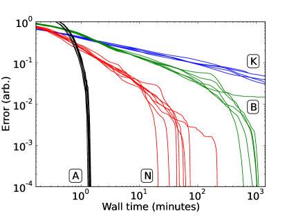
Figure 5: Corresponding to Fig. 1 from the main text, here for our second test problem. Performance comparison between several runs of the Newton-Raphson (red, labeled ‘N’), BFGS GRAPE (green, labeled ‘B’) and Krotov (blue, labeled ‘K’) algorithms with moderately sized initial pulses $\|\text{{{f}}}^{\left(0\right)}\|=20$. Also shown (in black, labeled ‘A’) are Newton-Raphson runs preceded by a routine to find the norm with least ill-conditioning.

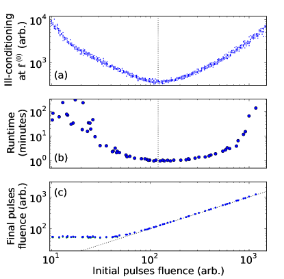
Figure 6: Direct analogue for our second test problem of Fig. 2 from the main text. For Newton-Raphson runs with initial pulses $\text{{{f}}}^{\left(0\right)}$ of different norms, (b) the wall time needed to reach an error $\varepsilon$ of $10^{-4}$ and (c) the norm of the corresponding solution pulses, with a dashed ‘initial equals final’ line. In addition, (a) the ill-conditioning of the Jacobian at several randomly sampled pulses of each norm.

As a second test problem, we can consider implementing a logical T-gate encoded with the five physical qubit stabilizer code as described in nigmatullin_implementation_2009_sup . The underlying system is a Heisenberg spin chain of length five, with a fixed external coupling field at a Rabi frequency of $10$, so that $H_{0}$ reads

$$\sum_{n=1}^{4}\sigma_{x}^{\left(n\right)}\sigma_{x}^{\left(n+1\right)}+\sigma_{y}^{\left(n\right)}\sigma_{y}^{\left(n+1\right)}+\sigma_{z}^{\left(n\right)}\sigma_{z}^{\left(n+1\right)}+10\sum_{n=1}^{5}\sigma_{x}^{\left(n\right)}$$

with an evolution time $T=90$. This has a single control corresponding to $H_{1}=\sigma_{z}^{\left(1\right)}$ enabling the first spin to be detuned, through a local voltage which is piecewise constant over $K=1500$ intervals.

References

- (1) H. M. Wiseman and G. J. Milburn. Quantum measurement and control. (Cambridge University Press, 2009)
- (2) M. Shapiro and P. Brumer. Principles of the quantum control of molecular processes. (Wiley-Interscience, 2003)
- (3) J. P. Dowling and G. J. Milburn. Phil. Trans. R. Soc. London A, 361, 1655 (2003)
- (4) H. Mabuchi and N. Khaneja. Int. J. Robust & Nonlin. Cont., 15, 647 (2005)
- (5) C. Brif, R. Chakrabarti, and H. Rabitz. New J. Phys., 12, 075008 (2010)
- (6) K. Singer, U. Poschinger, M. Murphy, P. Ivanov, F. Ziesel, T. Calarco, and F. Schmidt-Kaler. Rev. Mod. Phys., 82, 2609 (2010)
- (7) D. J. Tannor and S. A. Rice. J. Chem. Phys., 83, 5013 (1985)
- (8) T. Schulte-Herbrüggen, A. Spörl, N. Khaneja, and S. J. Glaser. Phys. Rev. A, 72, 042331 (2005)
- (9) A. M. Steane. Phys. Rev. A, 68, 042322 (2003)
- (10) F. Motzoi, J. M Gambetta, S. T Merkel, and F. K Wilhelm. arXiv:1102.0584, (2011)
- (11) P. K. Higuchi and S. Karp. U.S. Patent 3384715 (1968)
- (12) J.-S. Li, J. Ruths, T.-Y. Yu, H. Arthanari, and G. Wagner. P. Nat. Acad. Sci., 108, 1879 (2011)
- (13) V. Jurdjevic and H. J. Sussmann. J. Diff. Eq., 12, 313 (1972)
- (14) T. Caneva, M. Murphy, T. Calarco, R. Fazio, S. Montangero, V. Giovannetti, and G. E. Santoro. Phys. Rev. Lett., 103, 240501 (2009)
- (15) P. de Fouquieres, S. G. Schirmer, S. J. Glaser, and I. Kuprov. J. Mag. Res., 212, 412 (2011)
- (16) N. Khaneja, T. Reiss, C. Kehlet, T. Schulte-Herbrüggen, and S.J. Glaser. J. Mag. Res., 172, 296 (2005)
- (17) Y. Maday and G. Turinici. J. Chem. Phys., 118, 8191 (2003)
- (18) R Nigmatullin and S G Schirmer. New J. Phys., 11, 105032 (2009)
- (19) A. Spörl, T. Schulte-Herbrüggen, S. J. Glaser, V. Bergholm, M. J. Storcz, J. Ferber, and F. K. Wilhelm. Phys. Rev. A, 75, 012302 (2007)
- (20) I. Kuprov and C. T. Rodgers. J. Chem. Phys., 131, 234108 (2009)
- (21) C. T. Kelley. Solving nonlinear equations with Newton’s method. (SIAM, 2003)
- (22) A. Ben-Israel. J. Math. Anal. & Appl., 15, 243 (1966)
- (23) J. E Dennis and J. J Moré. Math. of Comp., 28, 549 (1974)
- (24) M.J.D. Powell. SIAM-AMS P. Nonlin. Prog., 9, 53 (1976)
- (25) D. H Li and M. Fukushima. SIAM J. Optim., 11, 1054 (2001)
- (26) P. Rebentrost, I. Serban, T. Schulte-Herbrüggen, and F. K. Wilhelm. Phys. Rev. Lett., 102, 090401 (2009)
- (27) J. Martínez. J. Comp. & Appl. Math., 34, 171 (1991)

References

- (1) J. Nocedal and S. J. Wright. Numerical Optimization. (Springer, New York, 1999)
- (2) S. Machnes, U. Sander, S. J. Glaser, P. de Fouquieres, A. Gruslys, S. G. Schirmer, and T. Schulte-Herbrüggen. Phys. Rev. A, 84, 022305 (2011)
- (3) A. Griewank. Math. Prog., 50, 141 (1991)
- (4) M. J. D. Powell. P. Int. Congr. Math., 1525 (1983)
- (5) M. J. D. Powell. Math. Prog., 11, 42 (1976)
- (6) D. C. Liu and J. Nocedal. Math. Prog., 45, 503 (1989)
- (7) H. Akaike. Ann. Inst. Stat. Math., 11, 1 (1959)
- (8) A. Ben-Israel. J. Math. Anal. & Appl., 15, 243 (1966)
- (9) S. Helgason. Differential geometry, Lie groups, and symmetric spaces. (Academic Press, New York, 1981)
- (10) V. Jurdjevic and H. J. Sussmann. J. Diff. Eq., 12, 313 (1972)
- (11) F. Kang and S. Zai-jiu. Numerische Mathematik, 71, 451 (1995)
- (12) A. Arvanitogeórgos. An introduction to Lie groups and the geometry of homogeneous spaces. (AMS Bookstore, 2003)
- (13) H. Federer. Geometric measure theory. (Springer, 1996)
- (14) A. Iserles, S. P. Nørsett, and A. F. Rasmussen. Appl. Numer. Math. 39, 379 (2001)
- (15) J. J. Moré and D. C. Sorensen. SIAM J. Sci. & Stat. Comp., 4, 553 (1983)
- (16) R Nigmatullin and S G Schirmer. New J. Phys., 11, 105032 (2009)