UK/12-02

Non-equilibrium Dynamics of $O(N)$ Nonlinear Sigma models: a Large-$N$ approach
Sumit R. Das^a and Krishnendu Sengupta^b

^aDepartment of Physics and Astronomy,
University of Kentucky, Lexington, KY 40506, USA
^b Theoretical Physics Department,
Indian Association for the Cultivation of Science, Jadavpur, Kolkata-700032, India.

We study the time evolution of the mass gap of the $O(N)$ non-linear sigma model in $2+1$ dimensions due to a time-dependent coupling in the large-$N$ limit. Using the Schwinger-Keldysh approach, we derive a set of equations at large $N$ which determine the time dependent gap in terms of the coupling. These equations lead to a criterion for the breakdown of adiabaticity for slow variation of the coupling leading to a Kibble-Zurek scaling law. We describe a self-consistent numerical procedure to solve these large-$N$ equations and provide explicit numerical solutions for a coupling which starts deep in the gapped phase at early times and approaches the zero temperature equilibrium critical point $g_{c}$ in a linear fashion. We demonstrate that for such a protocol there is a value of the coupling $g=g_{c}^{\rm dyn}>g_{c}$ where the gap function vanishes, possibly indicating a dynamical instability. We study the dependence of $g_{c}^{\rm dyn}$ on both the rate of change of the coupling and the initial temperature. We also verify, by studying the evolution of the mass gap subsequent to a sudden change in $g$, that the model does not display thermalization within a finite time interval $t_{0}$ and discuss the implications of this observation for its conjectured gravitational dual as a higher spin theory in $AdS_{4}$.

1 Introduction and Summary

The study of non-equilibrium dynamics of quantum field theories due to a time dependent mass or coupling has applications to many areas of physics. This has played a key role in our understanding of quantum field theory in cosmological backgrounds [1] and has, in recent years, been used as holographic descriptions of cosmological solutions in asymtptotically anti-de-Sitter spacetimes [2]. In condensed matter physics, the problem has received a lot of attention in recent times due to its experimental relevance to cold atom systems [3, 4, 5, 6, 7, 8, 9, 11]. There are several theoretical motivations to study this problem. One question relates to the issue of thermalization. Suppose we start with a field theory in its ground state. Now consider changing the coupling in time at some rate, eventually reaching some other constant value at late times. The question is : does the system reach a steady state at late times, and if so, does the steady state resemble a thermal state in any sense ?

Another issue involves the dynamics of a field theory when the time dependent coupling approaches or crosses an equilibrium critical point. This problem is of relevance to, and was initially studied in the context of, phase transitions in an expanding universe [10]. In this case, adiabaticity will be inevitably lost close to criticality and the subsequent dynamics will carry universal signatures of the critical point. For slow dynamics, a simple scaling hypothesis can indeed be used to show that several quantities such as density of excitations and excess energy scales with the rate of quench according some universal power-law which is determined solely by the universality class of the critical point [3]. Unlike equilibrium critical phenomena, there is no established theoretical framework to understand such universal behavior, and for strongly coupled field theories there are few theoretical tools to study this problem. Remarkable exceptions in this regard are systems in $1+1$ dimensions, where methods of boundary conformal field theory can be used to obtain results for correlation functions for an abrupt quench from a massive theory to a critical point[4, 5, 6, 7, 8]. It is thus important to accumulate as many “data points” as possible by examining individual models.

In this paper, we use large-N methods to study the non-equilibrium dynamics of the $O(N)$ Nonlinear Sigma Model in $2+1$ dimensions. We consider a time dependent coupling $g(t)=g_{i}+(g_{f}-g_{i})\tanh^{2}(vt)$ (where $v$ is the ramp rate and $g_{f}$ and $g_{i}$ are initial and final values of $g$) such that the system is initially, at $t=0$, in thermal equilibrium at a temperature $T$ in the disordered (paramagnetic) phase, and study the behavior of the mass gap of the model during and/or subsequent to this dynamics.

Using the Keldysh formalism, we show that at leading order in large $N$ the gap function is determined in terms of the time dependent coupling by a coupled set of differential and integral equations. For an initially slow variation of the coupling, a derivative expansion can be used to reduce these equations to a single inhomogeneous differential equation for the gap function, where the departure of the coupling from its equilibrium critical value acts as a source term. Near the critical point, adiabaticity breaks down. We determine the condition for breakdown of adiabaticity and show that it leads to a Kibble-Zurek type scaling relationship. We then describe a self-consistent numerical procedure to solve the coupled set of equations for arbitrary rates of change of coupling, and use this procedure to study the time dependence of the gap function as we approach close to the equilibrium critical point in the gapped phase. We find that the gap function always vanishes at a time $t_{0}$ where the instantaneous value of the coupling, $g(t_{0})=g_{c}^{\rm dyn}$ is larger than the equilibrium critical point at $T=0$, $g_{c}^{\rm eq}$. (We use the normalization of [12] where $g_{c}^{\rm eq}=1$.) We chart out the dependence of $g_{c}^{\rm dyn}$ on the ramp rate $v$ and the initial temperature $T$. We then study the evolution of the mass gap of the model subsequent to a sudden change in $g$ and verify that the system does not exhibit thermalization up to a time $t_{0}$ till which we can numerically track such an evolution. This result is consistent with known results about the lack of thermalization of vector models in the large-N limit [14] We comment on the consequence of such an absence of ”fast” thermalization (for $t\leq t_{0}$) of the gravity dual of this model. Finally, motivated by the derivative expansion, we study the problem for a Landau-Ginsburg dynamics and compare the time evolution with the $O(N)$ problem.

Large-$N$ quantum quench has been indirectly studied by using the AdS/CFT correspondence [15] to map large-$N$ limits of strongly coupled field theories to classical gravity. In these examples [16, 17, 18] (which involve $N\times N$ matrices, rather than $N$ component vectors), it is almost impossible to solve the field theory itself, but its dual gravity description is tractable. In contrast, the dual formulation of the 2+1 dimensional $O(N)$ vector model has been conjectured in [19] to be a higher spin gauge theory in $AdS_{4}$ [20] which contains an infinite number of massless higher spin fields. This conjecture has been explored in may papers, see in particular [21, 22] . In this case the field theory is tractable, and it will be interesting to see if this teaches us anything about quench and in particular thermalization time of the higher spin theory, specifically because there is an explicit dual map [21].

Quantum quench in the large-$N$ expansion has been studied earlier for the linear sigma model in [9] for infinitely fast quenches. This work does not deal with the issue of scaling behavior near the critical point. A similar work deals with BCS theory with an abruptly changing coupling [24]. In contrast, our work in the nonlinear model concentrates on the dependence of quench dynamics on the rate of quench. The fact that $g_{dyn}$ is larger than $g_{c}$ is similar in spirit to the phenomeon of stimulated superconductivity found in [25] and studied in the AdS/CFT context in [26].

The plan of the rest of the paper is as follows. In Sec. 2, we use the Keldysh formalism to derive a set of equations which determine the time-dependent gap (which we call the gap function) in terms of the time dependent coupling. This is followed by Sec. 3 where we derive the condition for breakdown of adiabaticity for the model as we approach the equilibrium critical point. Next, we discuss the determination of $g_{dyn}$ of this model in Sec. 4. In Sec. 5 we discuss the time evolution of the mass gap subsequent to a sudden change of coupling. Sec. 6 contains concluding remarks. In the Appendix we study a Landau-Ginzburg dynamics related to the $O(N)$ problem.

2 The model and the gap equation

The action of the model is given by

$$S=\int d^{2}xdt\left[\frac{N}{2g(t)}(\partial_{\mu}{\vec{\phi}}({\vec{x}},t))\cdot(\partial^{\mu}{\vec{\phi}}({\vec{x}},t))+\lambda({\vec{x}},t)[{\vec{\phi}}\cdot{\vec{\phi}}-1]\right]$$ (1)

where ${\vec{\phi}}({\vec{x}},t)$ is a $N$ dimensional vector with real components. In the large $N$ limit, $N\rightarrow\infty$ with $g(t)$ remaining $O(1)$.

The field $\lambda({\vec{x}},t)$ is a Lagrange multiplier which imposes the constraint ${\vec{\phi}}({\vec{x}},t)\cdot{\vec{\phi}}({\vec{x}},t)=1$. Redefining fields

$${\vec{\phi}}\rightarrow{\vec{\psi}}=\sqrt{\frac{N}{g(t)}}{\vec{\phi}}$$ (2)

the lagrangian density becomes, up to a total derivative

$${\mathcal{L}}=\frac{1}{2}(\partial{\vec{\psi}})^{2}-\frac{1}{2}\Sigma({\vec{x}},t)\left({\vec{\psi}}^{2}-\frac{N}{g(t)}\right)+N\frac{\alpha(t)}{g(t)}$$ (3)

where

$$\alpha(t)=\frac{1}{4}\left[\frac{3}{2}\left(\frac{\dot{g}}{g}\right)^{2}-\left(\frac{\ddot{g}}{g}\right)\right],~{}~{}~{}~{}~{}~{}~{}~{}\frac{1}{2}\Sigma({\vec{x}},t)=\frac{g(t)}{N}\lambda({\vec{x}},t)+\alpha(t)$$ (4)

The last term in (3) is field independent and can be therefore ignored.

The partition function can be expressed in the Schwinger-Keldysh formalism as

$${\mathcal{Z}}=\int{\mathcal{D}}{\vec{\psi}}_{\pm}{\mathcal{D}}\Sigma_{\pm}~{}e^{i\left[S({\vec{\psi}}_{+},\Sigma_{+})-S({\vec{\psi}}_{-},\Sigma_{-})\right]}$$ (5)

where we have doubled all the fields as usual, and $S$ is the action for the lagrangian in (3). As is well known, the representation (5) is schematic [13]- one has to pay attention to the end point of the time contour. However these ”boundary” terms do not affect the saddle point equation, though these are important for evaluation of the partition function by the saddle point solution.

One can now integrate out the fields ${\vec{\psi}}_{\pm}$ leading to the effective action for $\Sigma_{\pm}$,

$$S_{eff}=N{\rm Tr}~{}\log(D^{-1})-N\int d^{2}xdt\frac{1}{g(t)}[\Sigma_{+}-\Sigma_{-}]$$ (6)

where $D$ is the propagator matrix whose inverse is

$$D^{-1}=\left(\begin{array}[]{cc}\partial^{2}-\Sigma_{+}&0\\ \vskip 6.0pt plus 2.0pt minus 2.0pt\cr 0&-\partial^{2}+\Sigma_{-}\end{array}\right)$$ (7)

The large-N saddle point equations therefore become

$$\frac{1}{g(t)}={\rm Tr}~{}D_{++},~{}~{}~{}~{}~{}~{}~{}\frac{1}{g(t)}={\rm Tr}~{}(-D_{--})$$ (8)

Therefore, the saddle has $\Sigma_{+}=\Sigma_{-}\equiv\Sigma(t)$ and the equation becomes

$$\frac{1}{g(t)}=\int d^{2}x~{}<{\vec{x}},t|D|{\vec{x}},t>_{\beta}$$ (9)

where we are considering the problem at a temperature $T=1/\beta$. Note that the equality of $\Sigma_{+}$ and $\Sigma_{-}$ is a feature of the strict $N=\infty$ limit. Fluctuations around the saddle point will destroy this equality.

The coincident Green’s function in (9) may be obtained by considering a Heisenberg picture field which satisfies the homogeneous equation

$$[-\partial_{t}^{2}+\partial_{i}^{2}-\Sigma(t)]\chi({\vec{x}},t)=0.$$ (10)

Using a mode decomposition

$$\chi({\vec{x}},t)=\int\frac{d^{2}k}{(2\pi)^{2}}[a_{k}\chi_{k}(t)+a^{\dagger}_{k}\chi_{k}^{\star}(t)]$$ (11)

the equal time Green’s function $<\chi({\vec{x}},t)\chi({\vec{x}}^{\prime},t)>_{\beta}$ is the two point function in the thermal state, i.e. in the state

$$<a_{k}^{\dagger}a_{k}>_{\beta}=\frac{1}{e^{\beta\omega_{0}}-1}~{}~{}~{}~{}~{}~{}<a_{k}a^{\dagger}_{k}>_{\beta}=1+\frac{1}{e^{\beta\omega_{0}}-1}$$ (12)

where

$$\omega_{0}\equiv\sqrt{{\vec{k}}^{2}+\Sigma(0)}$$ (13)

The solution $\chi_{k}(t)$ may be written in the form

$$\chi_{k}(t)=\frac{1}{\sqrt{2\Omega_{k}(t)}}e^{-i\int^{t}\Omega_{k}(t^{\prime})dt^{\prime}}$$ (14)

where $\Omega_{k}(t)$ satisfies the equation

$$\frac{1}{2}\frac{\ddot{\Omega}_{k}}{\Omega_{k}}-\frac{3}{4}\left(\frac{\dot{\Omega}_{k}}{\Omega_{k}}\right)^{2}+\Omega_{k}^{2}=k^{2}+\Sigma(t)$$ (15)

Then the gap equation (9) becomes

$$\frac{1}{g(t)}=\int\frac{d^{2}k}{(2\pi)^{2}}\frac{1}{2\Omega_{k}(t)}\coth(\frac{\beta\omega_{0}}{2})$$ (16)

Note that the exponential factor in (14) canceled in the expression for the coincident time Green’s function.

The equation (16) has to be solved for $\Omega_{k}(t)$ for a given $g(t)$ and substitution of the solution in (15) gives the gap function $\Sigma(t)$.

Before ending this section, we note that for a time independent coupling $g_{0}$, our formalism reproduces the well-known equilibrium solution [12]. In this case, equation (15) shows that $\Omega_{k}=k^{2}+\Sigma$ i.e. the gap is now independent of time. The integral over $k$ on the right hand side yields the result

$$h_{0}(\beta)\equiv 2\pi\left(\frac{1}{g_{c}(\beta)}-\frac{1}{g_{0}}\right)=\frac{2}{\beta}\log\left[2\sinh(\frac{\beta}{2}\sqrt{\Sigma_{0}})\right]$$ (17)

Here $g_{c}(\beta)$ is given by

$$\frac{2\pi}{g_{c}(\beta)}=\frac{2}{\beta}\log\left[2\sinh(\frac{\beta\Lambda}{2})\right]$$ (18)

and $\Lambda$ is the momentum space UV cutoff. The equation (17) can be solved for $\Sigma_{0}$

$$\sqrt{\Sigma_{0}}=\frac{2}{\beta}\log\left[\frac{1}{2}e^{\beta h_{0}/2}+\frac{1}{2}\sqrt{e^{\beta h_{0}}+4}\right]$$ (19)

For any non-zero temperature this equation has a solution. At exactly zero temperature the gap equation becomes

$$h_{0}=\sqrt{\Sigma_{0}}$$ (20)

so that a real solution exists only for $g_{0}>g_{c}$. For $g_{0}<g_{c}$ the $O(N)$ symmetry is spontaneously broken and the theory is massless. The large-N solution presented above is not valid in this phase, though a valid solution in this phase is well known [12]. The point $g_{0}=g_{c}$ is then a critical point which separates the ordered and the massive phase. At non-zero temperatures, the critical point becomes a cross-over which separates regions of the phase diagram which are qualitatively similar to the ordered and the disordered phases. The location of the cross-over point is given by $\beta\sqrt{\Sigma_{0}}\sim 1$ which implies $h_{0}\sim T$ for small $T$.

3 Quantum Quench : Breakdown of Adiabaticity

When the coupling $g(t)$ varies slowly compared to the mass scale set by the coupling itself, one expects that the gap function $\Sigma(t)$ evolves adiabatically. Adiabaticity should break down when the gap function becomes small, e.g. near the zero temperature critical point. Let us define

$$h(t)\equiv 2\pi(\frac{1}{g_{c}(\beta)}-\frac{1}{g(t)})$$ (21)

To investigate adiabaticity, we first need to find an expansion for $\Omega_{k}(t)$ in terms of a $\Sigma(t)$ by solving (15) in a derivative expansion. This is easily done, and the lowest order result is

$$\frac{1}{\Omega_{k}(t)}=\frac{1}{\sqrt{k^{2}+\Sigma(t)}}+\frac{\ddot{\Sigma}}{8(k^{2}+\Sigma(t))^{5/2}}-\frac{5\dot{\Sigma}^{2}}{32(k^{2}+\Sigma(t))^{7/2}}+\cdots$$ (22)

We then need to substitute this in (16).

For zero temperature, it is possible to perform the necessary integrals and the lowest order result is

$$h(t)=\sqrt{\Sigma(t)}-\frac{1}{24}\frac{\ddot{\Sigma}}{\Sigma^{3/2}}+\frac{1}{32}\frac{\dot{\Sigma}^{2}}{\Sigma^{5/2}}+\cdots$$ (23)

Inverting this (again in a derivative expansion) we get

$$\sqrt{\Sigma(t)}=h(t)+\frac{1}{12h(t)}\left(\frac{\ddot{h}}{h}-\frac{1}{2}[\frac{\dot{h}}{h}]^{2}\right)+\cdots$$ (24)

Therefore adiabaticity breaks down when

$$|\frac{\ddot{h}}{h}-\frac{1}{2}[\frac{\dot{h}}{h}]^{2}|\sim h^{2}$$ (25)

We will be interested in generic profiles of $g(t)$ for which $h(t)\sim vt$ near $t=0$, e.g. $h(t)=-a\tanh(vt)$ for some dimensional parameter $a$. For such a profile adiabaticity breaks at a time

$$t_{\star}\sim v^{-1/2}$$ (26)

which is the usual Kibble-Zurek scaling for linear quenches.

These result trivially extends to nonlinear quenches. We note that the breakdown of adiabaticity can be also investigated analytically for low temperatures and the results are qualitatively similar up to exponentially small corrections.

4 Numerical Results for a Dynamical Instability

In this section, we determine the value of the coupling where the gap function first becomes zero. This possibly signals a dynamical instability. The protocol for $h(t)$ that we follow for studying this phenomenon is the following: we start with a fixed $g=g_{i}$ inside the disordered phase and with an equilibrium temperature $T$ and decrease $g$ to $g_{f}<g_{i}$ at the end of the evolution with a speed $v$. In the following we will take $g_{i}=4$ in all the calculations. This protocol is realized using

$$g(t)=g_{i}+(g_{f}-g_{i})\tanh^{2}(vt)$$ (27)

In what follows, we track the time evolution of the gap $\Sigma(t)$ and focus on finding the largest value of $g_{f}$ for which the minimum value of the mass gap, $\Sigma_{\rm min}$, reaches zero at some point during the evolution. This value yields $g_{c}^{\rm dyn}$. Since the numerical solution of the gap equation becomes difficult when $\Sigma_{\rm min}\to 0$, we extract the position of the dynamical critical point by extrapolation of $\Sigma_{\rm min}$ as a function of $g_{f}$. To elaborate, for each $v$, we let the system evolve from $g_{i}$ to $g_{f}$. We vary $g_{f}$ and approach the static critical point till it becomes difficult to obtain numerical convergence. We plot $\Sigma_{min}$ as a function of $g_{f}$ for a given $v$ and extrapolate this data to find $g_{dyn}$, i.e., value of $g_{f}$ for which $\Sigma_{min}$ reaches zero. We note at the outset that we have checked that the curve fitting based on such extrapolation typically generated correlation coefficient $R\geq 0.99$ and standard deviation $\sigma\leq 0.007$ which shows that errors from such a procedure are minimal.

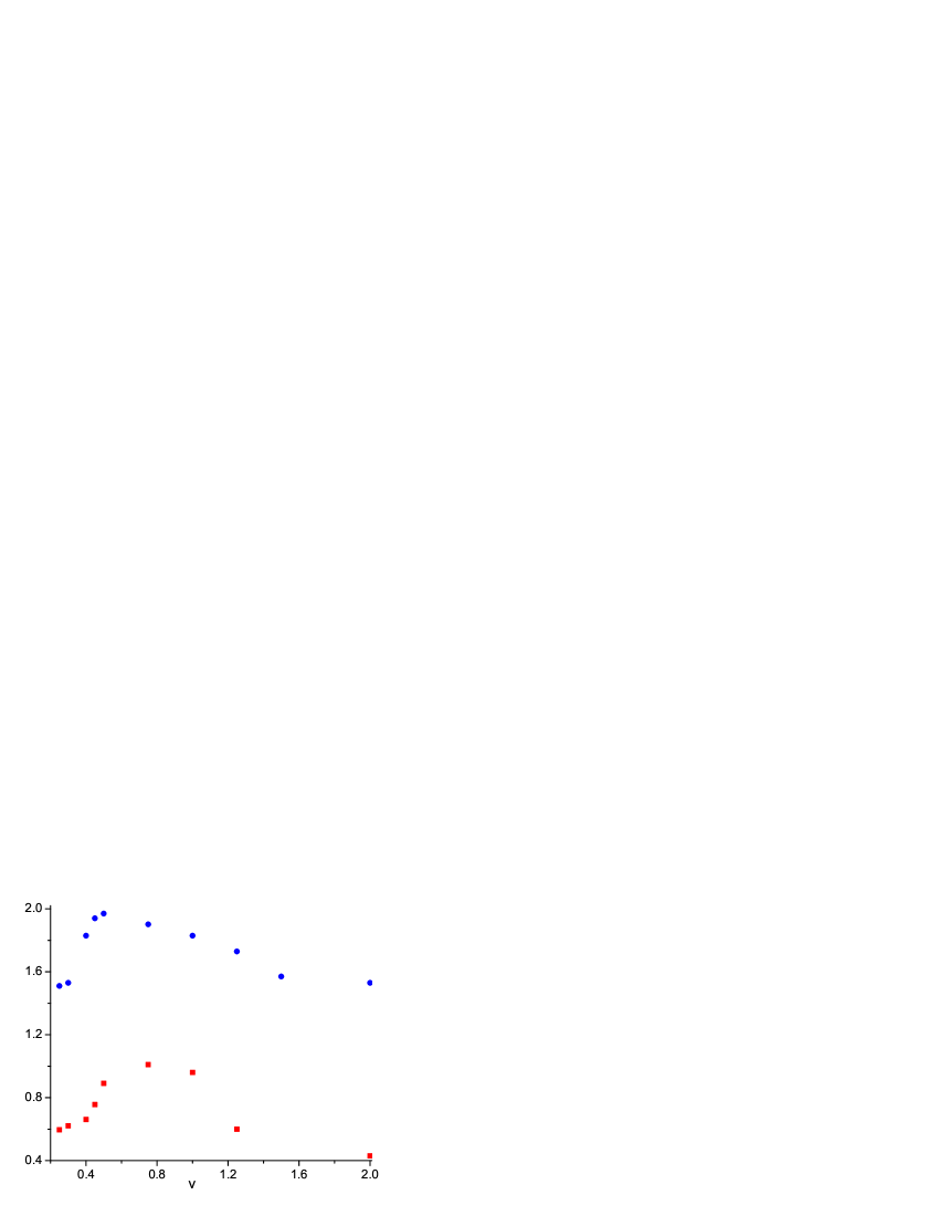
Figure 1: Rate dependence of $g_{c}^{\rm dyn}-1$ for $T=2$ (red square) and $g_{c}^{\rm dyn}$ for $T=1.75$ (blue circle). The shift in the value of $g_{c}^{\rm dyn}$ for $T=2$ is carried out to enhance clarity.

The numerical procedure we adopt for obtaining $\Sigma_{\rm min}$ for a given $v$ and $g_{f}$ is as follows. First, we provide initial guess values of $\Sigma(t)$ for a discrete set of points $t=t_{i}$ and numerically solve Eq. 15 to obtain $\Omega(k_{i},t_{i})$ for an array of discrete $k_{i}$ and $t_{i}$. From these values, using interpolation, we compute the $k$ integral appearing in the right side of Eq. 16 and obtain a set of trial values $g_{\rm trial}(t_{i})$. We then minimize the function $[g(t_{i})-g_{\rm trial}(t_{i})]^{2}$ self-consistently by varying $\Sigma(t_{i})$. We note here that the interpolation was carried out by choosing a set $N=21$ points. We have repeated some of our calculations with $N=31$ and $N=41$ points and have found that the values of $\Sigma(t_{i})$ obtained do not change to three decimal places. Thus the error bar in the data from finite size of $N$ is minimal.

The results of this procedure is summarized in Figs. 1 and 2. We find that for all rates $v\geq 0.25$ and temperatures $T\geq 0.05$ that we have studied, the gap function first touches zero at $g=g_{c}^{\rm dyn}>g_{c}=1$. The fact that $g_{dyn}$ is larger than $g_{c}$ is similar in spirit to the phenomenon of stimulated superconductivity found in [25] and studied in the AdS/CFT context in [26]. We find from Fig. 1 that the value of $g_{c}^{\rm dyn}$ increases with increasing $v$, reaches a maximum around a critical rate $v^{\ast}$ which depends on the starting equilibrium temperature, and then decreases as $v$ is further increased. We find $v^{\ast}$ reduces with decreasing temperature and the hump flattens.

The existence of $v^{\ast}$ can be qualitatively understood as follows. Since very slow dynamics in the disordered regime is expected to be adiabatic, we expect $g_{c}^{\rm dyn}$ to approach $g_{c}$ for small $v$. On increasing $v$, $g_{c}^{\rm dyn}$ increases and deviates from $g_{c}$. This continues till a rate $v=v^{\ast}$ after which the system does not have enough time to respond to the drive leading to a decrease in $g_{c}^{\rm dyn}$ with increasing $v$. Note that here we have restricted our numerics to values of $v$ so that the system reaches $g_{f}$ around $t=t_{0}$ till which we track the dynamics. For faster $v$ and fixed $t_{0}$, the system will eventually enter the quench regime where $g_{c}^{\rm dyn}$ will be determined by the evolution of $\Sigma(t)$ with $g=g_{f}$ subsequent to the quench till $t=t_{0}$. We do not address this regime in this section.

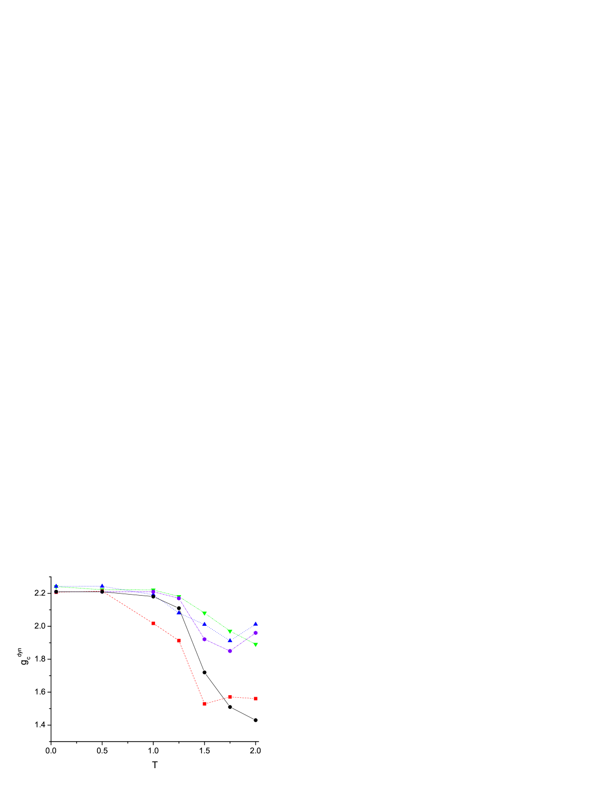
Figure 2: Temperature dependence of $g_{c}^{\rm dyn}$ for $v=2$ (black circle), $1.5$ (red square), $1.0$ (violet hexagon), $0.75$ (blue triangle), and $0.5$ (green inverted triangle).

The temperature dependence of $g_{c}^{\rm dyn}$ for different $v$ is shown in Fig. 2. Here we find that there is a crossover regime around $T=1$ where the behavior of $g_{c}^{\rm dyn}$ changes from the high temperature region where it shows appreciable variation with $v$ to a low temperature regime where it becomes virtually independent of $v$. Note that the saturation of $g_{c}^{\rm dyn}$ for small $v$ is consistent with the shifting of $v^{\ast}$ to lower values with decreasing temperature.

We end this section by noting that the dynamical instability of the time-dependent mass gap studied above need not correspond to a phase transition since the nature of the correlators of theory at the point where the time dependent mass gap vanish need not be long-range due to memory effects incorporated in $\Omega_{k}(t)$. It would be interesting to study such correlators near the instability; presently the slow convergence of the numerical solution near the instability prevents us from carrying out such a detailed study.

5 Time evolution after a sudden quench

In this section. we discuss the time evolution of the mass gap $\Sigma(t)$ subsequent to a sudden impulse imparted to the system. The impulse is imparted by changing $g(t)$ as $g(t)=(g_{i}-g_{d})+g_{d}\tanh^{2}[v(t-t_{1})]$ with $g_{i}=4$, $g_{d}=1$, $t_{1}=1$ and $v=20$. Note that with this choice, the system starts its evolution with $g=g_{i}$ at $t=0$. Near $t=t_{1}$, the coupling $g$ changes to $g_{f}=g_{i}-g_{d}$ and back to $g_{i}$. The change takes place within a time window of $\tau\sim 1/v$ around $t_{1}$ and thus appear as an instantaneous impulse for large $v$. The plot of the subsequent evolution of $\Sigma$ is plotted as a function of time in Fig. 3 for several initial temperatures. We note that for all temperatures, the system does not show any sign of thermalization in the sense that $\Sigma(t)$ does not approach any constant steady-state values till the time $t_{0}=10$ that we track it’s evolution numerically.

We believe that this is a manifestation of the lack of thermalization in $O(N)$ vector models to leading order in $1/N$. We note that from our numerical result, we can not rule out thermalization of the system at longer times; however, the model certainly do not thermalize for $t\leq t_{0}$. This is consistent with the expectation that vector models do not thermalize at large $N$, which is due to the lack of quasiparticle scattering at $O(1/N)$. ( Such scattering in the present models appears in $O(1/N^{2})$ and ultimately leads to thermalization.) This is in contrast with large-N models of matrices, where thermalization is expected to occur [14] at the leading order . This is manifest for the class of such large-N models which have gravity duals, where thermalization is seen as formation of black holes [16]. In such models, thermalization is almost instantaneous for local operators.

This is also consistent with the fact that the gravity dual of the $O(N)$ model is a higher spin gauge theory rather than standard Einstein gravity. In usual $AdS/CFT$ duals of models of large-N matrices (e.g. gauge theories), thermalization is signalled by black hole formation. However, a study of the finite temperature properties of the singlet sector of the higher spin model shows that there is no large-N transition at order one temperatures [30]. This possibly implies the absence of thermodynamically stable large black holes with order one Hawking temperatures in this higher spin theory.

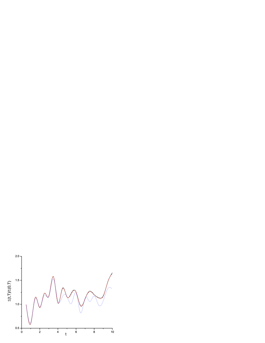
Figure 3: The evolution of the mass gap after a sudden quench at $t=1$ as a function of time till $t=t_{0}=10$ for temperatures $T=2$ (blue dotted line), $T=1$ (red dashed line) and $T=0.1$ (black solid line).

6 Conclusions

In conclusion, we have shown that the nonequlibirum dynamics of the non-linear O(N) sigma model with a time dependent coupling $g(t)$ is summarized by two coupled equations (15) and (16). Whenever a derivative expansion is valid, these equations can be reduced formally to a single differential equation for the gap function with arbitrarily higher derivatives, equation (23). This latter equation has been used to determine the condition of breakdown of adiabaticity at zero temperature : this led to Kibble-Zurek scaling. We then described how these equations can be solved by a self-consistent numerical procedure. We presented numerical results for the case where the coupling which approaches a constant value deep in the paramagnetic region, and approaches the zero temperature equilibrium critical value in the future, starting with a thermal state. We found that during the time evolution, the instantaneous value of the gap reaches zero for a coupling $g_{dyn}$ which is larger than the coupling at the equilibrium critical point and studied the dependence of $g_{dyn}$ on the quench rate. Finally, we have studied the response of the model to a sudden quench and verified that the model does not exhibit short-time thermalization, and have discussed the consequence of this phenomenon for its gravity dual.

Our numerical procedure does not work well near $g=g_{dyn}$ which is the regime of obvious interest. We are working on different numerical procedures to overcome these difficulties.

It would be interesting to extend this approach to discuss the dynamics when the coupling crosses the critical point. This requires a treatment of the saddle point equations in the ordered phase as in [12]. Finally, our work can in principle be extended to a study of periodic dynamics. These questions are being currently investigated.

7 Acknowledgements

We are grateful to Ganpathy Murthy for extensive discussions and collaboration at the early stages of this work and for valuable comments about the manuscript. S.R.D. would like to thank Institut de Fisica Teorica at Madrid, Tata Institute of Fundamental Research at Mumbai, Indian Association for the Cultivation of Science at Kolkata and Kobayashi-Maskawa Institute in Nagoya for hospitality during the course of this work. This work is partially supported by National Science Foundation grants PHY-0970069 and PHY-0855614. KS thanks University of Kentucky for hospitality and DST, India for support through grant no. SR/S2/CMP-001/2009.

8 Appendix : Landau-Ginzburg Dynamics

Large N theories are classical in the leading order, and one might imagine that there is a classical equation of motion which describes this limit, typically in one higher dimension. Models of $N\times N$ matrices are often of this type, e.g. matrix quantum mechanics whose large-N limit is described by the classical equations of $1+1$ dimensional string theory [27] - the string field in this case is in fact a single massless scalar which can be identified with a suitable collective variable [28]. AdS/CFT dualities are also of this kind : the large-N classical theories are generically string theories in one higher dimension and contain an infinite number of fields. Nevertheless, usually in the strong coupling limit, only a few of these fields are massless (which is the statement that in the field theory only a few operators have dimensions of order one rather than of order $N$). In that case the dual theory is described by a finite number of classical equations of motion, viz. Einstein equations and equations of motion of a few other fields.

So long as the derivative expansion is valid, the gap function in our system satisfies an inhomogeneous differential equation (23) where the quantity $h(t)$ defined above acts as a source. This equation is valid in the disordered phase. In fact, in the general case where the lagrange multiplier field $\Sigma$ depends on both space and time, this is one of the collective fields which describe the large-N dynamics. Exactly at the critical point this is identified with the scalar field in $AdS_{4}$ Vasiliev theory [29]. Of course the equation (23) breaks down as we approach $h(t)=0$.

This motivates us to compare the nonequilibrium behavior of our $O(N)$ model with the non-equilibrium dynamics of a toy Landau-Ginzburg (LG) type model. The equation is given by

$$\frac{d^{2}\xi(t)}{dt^{2}}+c\frac{d\xi}{dt}+\xi^{3}+J(t)=0$$ (28)

The field $\xi$ is the analog of the gap function and $J(t)$ plays the role of the coupling $h(t)$ in the previous sections. A ”mass term” in this model has been set to zero to ensure that the equilibrium theory is critical when $J(t)=0$ and we have added a friction term with coefficient $c$ to account for dissipation.

Consider a time dependent source in (28) of the form

$$J(t)=J_{i}+(J_{f}-J_{i})\tanh^{2}(vt)$$ (29)

pretty much like $g(t)$ chosen for the $O(N)$ model. We now solve the equation for a fixed $J_{i}$, starting at $t=0$ with adiabatic initial conditions for different values of $J_{f}$, and determine the value of $J_{f}=J_{f}^{c}$ for which the order parameter $\xi$ first touches zero. A typical time evolution of the order parameter is shown in Figure(4) for vanishing friction and in Figure(5) in the presence of some friction.

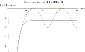
Figure 4: A typical behavior of the order parameter as a function of time, with the source function given by (29) and vanishing friction. The evolution starts from $t=0$. The purple line is the adiabatic value of the order parameter. The value of $J_{f}$ chosen in this plot corresponds to the dynamical critical point.

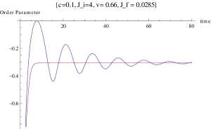
Figure 5: A typical behavior of the order parameter as a function of time, with the source function given by (29) and some friction. The evolution starts from $t=0$. The purple line is the adiabatic value of the order parameter. The value of $J_{f}$ chosen in this plot corresponds to the dynamical critical point.

Figure (6) shows the behavior of $J_{dyn}$ as a function of the ramp speed for vanishing friction. Figure (7) is the same plot in the presence of friction. For very small $v$, $J_{dyn}$ is very small and increasing with $v$ since the time evolution is expected to be adiabatic. For large $v$ we have a rapid quench. The system does not have enough time to react to the change and remains in the initial state for quite some time, after which it starts oscillating. $J_{dyn}$ saturates to a constant value.

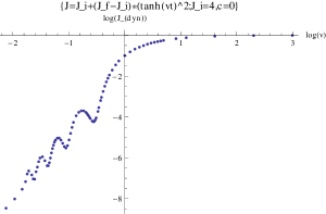
Figure 6: A log-log plot of $J_{dyn}$ versus $v$ with no friction. The saturation value is $\frac{1}{4}J_{i}$ as expected.

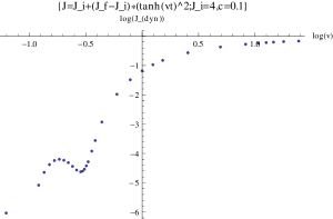
Figure 7: A log-log plot of $J_{dyn}$ versus $v$ with friction.

For vanishing friction, the saturation value may be understood as follows. For large $v$, the quench is rapid at $t=0$. We may then approximate $J(t)$ by $J(0)=J_{i}$ and $J(t)=J_{f}$ for $t>0$ . Then a first integral of the equation of motion (28) for $t>0$ is given by

$$\frac{1}{2}\left(\frac{d\xi}{dt}\right)^{2}+\frac{1}{4}\xi^{4}+J_{f}\xi=E$$ (30)

Since at $t=0$ the initial conditions are adiabatic $\xi(0)=[-J_{i}]^{1/3}$ and ${\dot{\xi}}(0)=0$, so that $E=\frac{1}{4}J_{i}^{4/3}-J_{f}J_{i}^{1/3}$. Now, at the time when the order parameter first touches zero, we must have $\xi=0$ and ${\dot{\xi}}=0$. For this to happen we must have $E=0$, i.e. $J_{f}=\frac{1}{4}J_{i}$. Indeed, we have checked that the saturation value of $J_{dyn}$ is indeed given by $\frac{1}{4}J_{i}$.

The behavior of $J_{dyn}$ as a function of $v$, however, displays non-monotonic behavior for intermediate $v$, with multiple well-defined humps. In the presence of friction we could not find multiple humps, but one hump always remains. We do not understand the reason behind this behavior. However, it is interesting that there is a similar behavior in the nonlinear sigma model, even though the latter differs significantly from our toy model when the gap vanishes at some time.

The presence of humps in the behavior of $J_{dyn}$ is intruigingly similar to similar non-monotonicity found in the $O(N)$ model. However, other aspects of these results appear to be quite different from our $O(N)$ results. In particular, while $J_{dyn}$ in the LG theory saturates at large speeds, the $g_{c}^{dyn}$ appears to first rise and then come closer to the equilibrium critical coupling $g_{c}=1$. It is conceivable that for much larger speeds, $g_{c}^{dyn}$ rises again and saturates. However, numerical convergence becomes difficult at high ramp speeds.

It is also conceivable that this difference reflects a fundamental difference between the large-N classical theory of $O(N)$ as formulated above and a LG type theory. As discussed above the gap function is not related to the coupling in a local fashion in time. The gap equation (16) relates $g(t)$ with $\Omega_{k}(t)$ which depends on the entire function $\Sigma(t)$ through the differential equation (15). It is only in the adiabatic approximation that the gap function satisfies a differential equation with a source given by the coupling - and adiabaticity of course fails when the gap function vanishes. This is related to the fact that this theory is dual to a theory of an infinite number of massless higher spin fields, and the gap function is simply one of these fields. This implies that an effective equation for the gap function would be non-local. It would be interesting to see if the bilocal collective field theory approach to this duality [21] can shed any light on this issue.

References

- [1] N. D. Birrell and P. C. W. Davies, “Quantum Fields In Curved Space,” Cambridge, Uk: Univ. Pr. ( 1982) 340p
- [2] S. R. Das, J. Michelson, K. Narayan and S. P. Trivedi, “Time dependent cosmologies and their duals,” Phys. Rev. D 74, 026002 (2006) [hep-th/0602107]; C. -S. Chu and P. -M. Ho, “Time-dependent AdS/CFT duality and null singularity,” JHEP 0604, 013 (2006) [hep-th/0602054]; S. R. Das, “Gauge-gravity duality and string cosmology,” In *Erdmenger, J. (ed.): String cosmology* 231-265
-
[3]
For a review see S. Mondal, D. Sen and K. Sengupta,
“Non-equilibrium dynamics of quantum systems: order parameter
evolution, defect generation, and qubit transfer,” Chap 2 in
”Quantum Quenching, Annealing and Computation”, Eds. A. Das, A.
Chandra and B. K. Chakrabarti, Springer Lect. Notes Phys.,
802, 21 (2010) [arXiv:0908.2922];
J. Dziarmaga, ”Dynamics of a Quantum Phase Transition and Relaxation to a Steady State” Adv. Phys. 59, 1063 (2010) [arXiv:0912.4034];
A. Polkovnikov, K. Sengupta, A. Silva and M. Vengalattore, ”Nonequilibrium dynamics of closed interacting quantum systems”, Rev. Mod. Phys. 83 863 (2011) [arxiv:1007.5331]. - [4] P. Calabrese and J. L. Cardy, “Evolution of Entanglement Entropy in One-Dimensional Systems,” J. Stat. Mech. 0504 (2005) P010 [arXiv:cond-mat/0503393].
- [5] P. Calabrese and J. L. Cardy, “Time-dependence of correlation functions following a quantum quench,” Phys. Rev. Lett. 96 (2006) 136801 [arXiv:cond-mat/0601225].
- [6] P. Calabrese and J. Cardy, “Quantum Quenches in Extended Systems,” [arXiv:0704.1880 [cond-mat.stat-mech]].
- [7] S. Sotiriadis and J. Cardy, “Inhomogeneous Quantum Quenches ,” J. Stat. Mech. (2008) P11003, [arXiv:0808.0116 [cond-mat.stat-mech]].
- [8] S. Sotiriadis, P. Calabrese and J. Cardy, “Quantum Quench from a Thermal Initial State” EPL 87 (2009) 20002, [arXiv:0903.0895 [cond-mat.stat-mech]].
- [9] S. Sotiriadis and J. Cardy, “Quantum quench in interacting field theory: a self-consistent approximation,” arXiv:1002.0167 [quant-ph].
- [10] T. W. B. Kibble, J. Phys. A A 9, 1387 (1976); W. H. Zurek, Nature 317, 505 (1985).
-
[11]
A. Polkovnikov, “Universal adiabatic dynamics in the
vicinity of a quantum critical point,” Phys. Rev. B72
(2005) 161201 [arXiv:cond-mat/0312144];
A. Polkovnikov and V. Gritsev , “Universal Dynamics Near Quantum Critical Points,” Nature Physics 4, 477 (2008)[arXiv: 0910.3692];
K. Sengupta, D. Sen and S. Mondal, “Exact results for quench dynamics and defect production in a two-dimensional model,” Phys. Rev. Lett. 100 (2008) 077204 [arXiv:0710.1712]; D. Sen, K. Sengupta, S. Mondal, ” Defect Production in Nonlinear Quench across a Quantum Critical Point”, Phys. Rev. Lett. 101 (2008) 016806 [arXiv:0803.2081]
D. Patane, L. Amico, A. Silva, R. Fazio and G. Santoro, “Adiabatic dynamics of a quantum critical system coupled to an environment: Scaling and kinetic equation approaches” Phys. Rev. B80 (2009) 024302 [arXiv:0812.3685]. - [12] S. Sachdev, Quantum Phase Transitions (Cambridge University Press, Cambridge, England, 1999).
- [13] A. Kamenev and A. Levchenko, ”Keldysh technique and non-linear sigma-model: basic principles and applications”, Adv. Phys. 58 (2009) 197.
- [14] G. Festuccia and H. Liu, “The Arrow of time, black holes, and quantum mixing of large N Yang-Mills theories,” JHEP 0712, 027 (2007) [hep-th/0611098]; N. Iizuka and J. Polchinski, “A Matrix Model for Black Hole Thermalization,” JHEP 0810, 028 (2008) [arXiv:0801.3657 [hep-th]].
- [15] J. M. Maldacena, “The large N limit of superconformal field theories and supergravity,” Adv. Theor. Math. Phys. 2 (1998) 231 [Int. J. Theor. Phys. 38 (1999) 1113] [arXiv:hep-th/9711200]; S. S. Gubser, I. R. Klebanov and A. M. Polyakov, “Gauge theory correlators from non-critical string theory,” Phys. Lett. B 428, 105 (1998) [arXiv:hep-th/9802109]; E. Witten, “Anti-de Sitter space and holography,” Adv. Theor. Math. Phys. 2, 253 (1998) [arXiv:hep-th/9802150].
- [16] R. A. Janik and R. B. Peschanski, “Gauge / gravity duality and thermalization of a boost-invariant perfect fluid,” Phys. Rev. D 74, 046007 (2006) [arXiv:hep-th/0606149]; R. A. Janik, “Viscous plasma evolution from gravity using AdS/CFT,” Phys. Rev. Lett. 98, 022302 (2007) [arXiv:hep-th/0610144]; P. M. Chesler and L. G. Yaffe, “Horizon formation and far-from-equilibrium isotropization in supersymmetric Yang-Mills plasma,” Phys. Rev. Lett. 102, 211601 (2009) [arXiv:0812.2053 [hep-th]]; P. M. Chesler, L. G. Yaffe, “Boost invariant flow, black hole formation, and far-from-equilibrium dynamics in N = 4 supersymmetric Yang-Mills theory,” Phys. Rev. D82, 026006 (2010). [arXiv:0906.4426 [hep-th]]; S. Bhattacharyya and S. Minwalla, “Weak Field Black Hole Formation in Asymptotically AdS space-times,” JHEP 0909 (2009) 034 [arXiv:0904.0464 [hep-th]].
- [17] S. R. Das, T. Nishioka, T. Takayanagi, “Probe Branes, Time-dependent Couplings and Thermalization in AdS/CFT,” JHEP 1007, 071 (2010). [arXiv:1005.3348 [hep-th]].
- [18] P. Basu and S. R. Das, JHEP 1201, 103 (2012) [arXiv:1109.3909 [hep-th]].
- [19] I. R. Klebanov, A. M. Polyakov, “AdS dual of the critical O(N) vector model,” Phys. Lett. B550, 213-219 (2002). [hep-th/0210114]
- [20] See e.g. M. A. Vasiliev, “Higher spin gauge theories in various dimensions,” Fortsch. Phys. 52, 702 (2004) [hep-th/0401177].
- [21] S. R. Das, A. Jevicki, “Large N collective fields and holography,” Phys. Rev. D68, 044011 (2003). [hep-th/0304093]; R. d. M. Koch, A. Jevicki, K. Jin, J. P. Rodrigues, “ Construction from Collective Fields,” Phys. Rev. D83, 025006 (2011). [arXiv:1008.0633 [hep-th]].
- [22] S. Giombi, X. Yin, “Higher Spin Gauge Theory and Holography: The Three-Point Functions,” JHEP 1009, 115 (2010). [arXiv:0912.3462 [hep-th]].
- [23] E. Sezgin and P. Sundell, Nucl. Phys. B 644, 303 (2002) [Erratum-ibid. B 660, 403 (2003)] [hep-th/0205131].
- [24] R. Barankov, L. Levitov and B. Spivak, Phys. Rev. Lett. 93, 160401 (2004) [arXiv:cond-mat/0312053].
- [25] G.M. Eliashberg, JETP Lett. 11 (1970) 114.
- [26] N. Bao, X. Dong, E. Silverstein and G. Torroba, “Stimulated superconductivity at strong coupling,” JHEP 1110, 123 (2011) [arXiv:1104.4098 [hep-th]].
- [27] E. Brezin and V. A. Kazakov, “Exactly Solvable Field Theories Of Closed Strings,” Phys. Lett. B 236, 144 (1990); D. J. Gross and N. Miljkovic, “A Nonperturbative Solution Of D = 1 String Theory,” Phys. Lett. B 238, 217 (1990); P. H. Ginsparg and J. Zinn-Justin, “2-d GRAVITY + 1-d MATTER,” Phys. Lett. B 240, 333 (1990).
- [28] S. R. Das and A. Jevicki, “String Field Theory And Physical Interpretation Of D = 1 Strings,” Mod. Phys. Lett. A 5, 1639 (1990).
- [29] S. Giombi and X. Yin, arXiv:1105.4011 [hep-th].
- [30] S. H. Shenker and X. Yin, “Vector Models in the Singlet Sector at Finite Temperature,” arXiv:1109.3519 [hep-th].
- [31] P. Buividovich, arXiv: 0903.4263.