First Results of a Detailed Analysis of
p+p Elastic Scattering Data from ISR to LHC Energies
in the Quark-Diquark Model

Abstract

First results of a detailed analysis of p+p elastic scattering data are presented from ISR to LHC energies utilizing the quark-diquark model of protons in a form proposed by Bialas and Bzdak. The differential cross-section of elastic proton-proton collisions is analyzed in detailed and systematic manner at small momentum transfers, starting from the energy range of CERN ISR at $\sqrt{s}=23.5$ GeV, including also recent TOTEM data at the present LHC energies at $\sqrt{s}=7$ TeV. These studies confirm the picture that the size of protons increases systematically with increasing energies, while the size of the constituent quarks and diquarks remains approximately independent of (or only increases only slightly with) the colliding energy. The detailed analysis indicates correlations between model parameters and also indicates an increasing role of shadowing at LHC energies.

1 Introduction

The differential cross section of elastic scattering of p+p collisions allows one to study the internal structure of protons using the theory of diffraction. Varying the momentum transfer one can change the resolution of the investigation: increasing the momentum transfer corresponds to looking more and more deeply inside the structure of protons. One of the fundamental outcomes of diffractive p+p scattering studies was the indication that protons have a finite size and a complicated internal structure, thus the protons can be considered as composite objects.

Our interest in this problem has been triggered by two factors: an interesting series of recent theoretical work and also new data from the TOTEM experiment at CERN LHC. These are detailed below. Recently, we became aware of an inspiring series of papers of Bialas, Bzdak and collaborators, who studied elastic proton-proton [1], pion-proton [2] and nucleus-nucleus collisions [3],[4] in a framework where the proton was considered as a composite object that contains correlated quark and diquark constituents. In this work, we confirm their main conclusion: the quark-diquark model of nucleon structure at low momentum transfer does capture the main features of this problem and indeed it deserves a closer, more detailed attention. This study is dedicated to a follow-up, more detailed investigation, not only including an estimation of the best values of the parameters, as was done in ref. [1], but also determining their errors and also the evaluation of the models based on an analysis of the presented fit quality. In order to reach these goals, we utilized standard experimental techniques, such as multi-parameter optimalization or fitting with the help of the MINUIT function minimalization and multi-parameter optimalization package [5].

In addition to these simple, straightforward and interesting theoretical investigations of elastic scattering data from CERN ISR in the energy range of $\sqrt{s}=$ 23.5, 30.7, 52.9 and 62.5 GeV, that were already analyzed in ref. [1], new elastic scattering data became available recently at $\sqrt{s}=7$ TeV [16] from the CERN LHC experiment TOTEM. So we have tested the model of Bialas and Bzdak not only at ISR energies but also at the currently available highest LHC energies on recent TOTEM data, in order to learn more details about the evolution of the properties of p+p elastic interactions in the recently opened, few TeV energy range.

Most of the arguments for the composite structure of hadrons have been derived from the studies of lepton-hadron interactions. The emerging standard picture is that hadrons are either mesons, composed of valence quarks and anti-quarks, or (anti)baryons, composed of three valence (anti)quarks, that carry the quantum numbers, while the electrically neutral gluons carry color charges and provide the binding among the quarks and anti-quarks. The exact contribution of quarks, gluons, and the sea of virtual quark-antiquark pairs and gluons to certain hadronic properties e.g. spin is still under detailed investigation. For example, the gluon contribution to the proton spin is still not fully constrained [6]. Also, more than 10 exotic hadronic resonances called X, Y and Z states were recently discovered in electron-positron collisions at the world’s highest luminosities in the BELLE experiment at KEK. These hadronic states cannot be interpreted in the standard picture of quark-antiquark or three (anti)quark bound states, according to refs. [7, 8] Thus even nowadays there are still several open questions that are related to the compositeness of the hadrons in general. As gluons do not interact with directly with leptons, their properties are best explored with the help of the strong hadronic interactions. For example, the gluon contribution to the proton spin is investigated with the help of polarized proton - polarized proton collisions at RHIC [6].

In this work, we focus on the effects of internal correlations between the quarks inside the protons, examining in detail proton-proton elastic scattering at several ISR and also at the currently maximal available LHC energies. Let us recall, that a similar analysis involving three independent quarks was not able to properly describe the ISR data  [9]. In that model quarks were considered as “dressed” valence quarks in the sense that they contain the gluonic and $q\bar{q}$ contribution as well, as if the glue would be concentrated around pointlike valence quarks. 30 years after the three independent quark model of ref. [9] another three-quark model of the protons was proposed in ref. [1], that included interesting correlations between two dressed valence quarks to form a diquark. This quark-diquark model [1], is the basis of our current study, in order to examine in details proton-proton elastic scattering at ISR and LHC energies.

The quark-diquark picture of elastic p+p scattering resembles to the Glauber optical model [12] in nuclear physics, where a multiple expansion is applied. The Glauber model, developed originally for nuclear multiple scattering problems like cross sections of protons and neutrons on deuteron, became a standard model of high energy interactions in nuclear physics where multiple interactions are built up from superpositions of nucleon-nucleon scattering. This model became a fundamental and successfull tool in describing nuclear collisions at high energy  [10].

The body of this manuscript is organized as follows: the theoretical models are described in Section 2, for both cases, when the diquark acts as a single entity and also when it acts as a composite object. In Section 3 the original results of Bialas and Bzdak are reproduced and detailed, including a note on the quality of these data descriptions. Section 4 contains our main new results, the first MINUIT results. The conclusion takes place in Section 5.

2 Elastic scattering in the quark-diquark model

We describe proton-proton interactions as collision of two systems, each one composed of a dressed quark and diquark. The collision is schematically illustrated on Fig. 1.

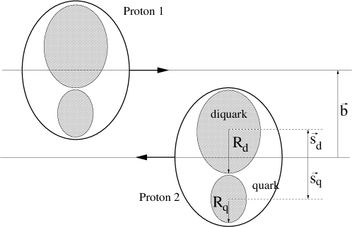
Figure 1: The schematic scattering situation of the two protons when the diquark is assumed to be a single entity.

The interaction between quarks and diquarks is assumed to be purely absorptive. Consequently the amplitude has no real part and the imaginary part – dominating at high energy – is given by the absorption of the incoming particle wave, namely the inelastic (non-diffractive) collisions.

In the impact parameter space the inelastic proton-proton cross-section for a fixed impact parameter $\vec{b}$ can be given by the following formula [1]

$$\sigma(\vec{b})=\int\limits^{+\infty}_{-\infty}...\int\limits^{+\infty}_{-\infty}{\text{d}^{2}s_{q}\text{d}^{2}s^{\prime}_{q}\text{d}^{2}s_{d}\text{d}^{2}s^{\prime}_{d}D(\vec{s_{q}},\vec{s_{d}})D(\vec{s_{q}}^{\prime},\vec{s_{d}}^{\prime})\sigma(\vec{s_{q}},\vec{s_{d}};\vec{s_{q}}^{\prime},\vec{s_{d}}^{\prime};\vec{b})},$$ (1)

where $\vec{s_{q}}$, $\vec{s_{q}}^{\prime}$ and $\vec{s_{d}}$, $\vec{s_{d}}^{\prime}$ are the transverse positions of the quarks and diquarks respectively, and the integrand is the probability function of having inelastic interaction at a given impact parameter $\vec{b}$ and transverse positions of the constituents.

The quark-diquark distribution inside the nucleon is taken into account with the following Gaussian

$$D\left(\vec{s_{q}},\vec{s_{d}}\right)=\frac{1+\lambda^{2}}{\pi R_{p}^{2}}e^{-(s_{q}^{2}+s_{d}^{2})/R_{p}^{2}}\delta^{2}(\vec{s_{d}}+\lambda\vec{s_{q}}),\;\lambda=m_{q}/m_{d},$$ (2)

where $R_{p}$ is the “proton size”, the variance of the distribution and $\lambda$ is the mass ratio of the quark and the diquark. Obviously $1/2\leq\lambda\leq 1$, where $1/2$ would indicate a loosely bound diquark. The two dimensional delta function preserves the center of mass in the tranverse plane.

Elastic interactions of the constituents are independent inside the proton, accordingly the probability distribution of elastic proton-proton collision is the product of the probability distribution of elastic interactions of the constituents [11, 13]

$$\sigma(\vec{s_{q}},\vec{s_{d}};\vec{s_{q}}^{\prime},\vec{s_{d}}^{\prime};\vec{b})=1-\prod_{a,b\in\{q,d\}}\{1-\sigma_{ab}(\vec{b}+\vec{s_{a}}^{\prime}-\vec{s_{b}}^{\prime})\}.$$ (3)

The inelastic differential cross-sections are parametrized with Gaussian distributions

$$\sigma_{ab}\left(\vec{s}\right)=A_{ab}e^{-s^{2}/R_{ab}^{2}},\;R_{ab}^{2}=R_{a}^{2}+R_{b}^{2},$$ (4)

where $R_{ab}$ is the variance of having an inelastic collision, which is calculated from the sum of the squared $R_{q}$, $R_{d}$ radius parameters; the $A_{ab}$ parameters are the ampitudes. From unitarity the elastic amplitude in impact parameter space

$$t_{el}(\vec{b})=1-\sqrt{1-\sigma(\vec{b})}.$$ (5)

The elastic amplitude in momentum transfer representation is the Fourier-transform of the amplitude in impact parameter space

$$T(\vec{\Delta})=\int\limits^{+\infty}_{-\infty}\int\limits^{+\infty}_{-\infty}{t_{el}(\vec{b})e^{i\vec{\Delta}\cdot\vec{b}}\text{d}^{2}b}=2\pi\int\limits_{0}^{+\infty}{t_{el}\left(b\right)J_{0}\left(\Delta b\right)b{\text{d}}b},$$ (6)

where $\Delta=|\vec{\Delta}|$, $b=|\vec{b}|$ and $J_{0}$ is the zeroth Bessel-function of the first kind. Then the elastic differential cross section reads as

$$\frac{d\sigma}{dt}=\frac{1}{4\pi}\left|T\left(\Delta\right)\right|^{2}.$$ (7)

2.1 The diquark is assumed to act as a single entity

The subject of this section is to analyse that case when the quark and diquark radii are independent model parameters, which means that the diquark is considered as one entity as indicated on Fig. 1. In this case, the number of free parameters can be reduced if we assume that the number of partons is twice as many in the diquark than in the quark. From the inelastic differential cross sections (4) the total inelastic cross sections are

$$\sigma_{ab}=\int\limits^{+\infty}_{-\infty}\int\limits^{+\infty}_{-\infty}{\sigma_{ab}\left(\vec{s}\right)}\text{d}^{2}s=\pi A_{ab}R_{ab}^{2},\;a,b\in\{q,d\}.$$ (8)

Our assumption tells us that

$$\sigma_{qq}:\sigma_{qd}:\sigma_{dd}=1:2:4,$$ (9)

from which we can deduce the following expressions

$$A_{qd}=A_{qq}\frac{4R_{q}^{2}}{R_{q}^{2}+R_{d}^{2}},\;A_{dd}=A_{qq}\frac{4R_{q}^{2}}{R_{d}^{2}},$$ (10)

which means that every $A_{ab}$ parameter can be expressed in term of $A_{qq}$. With these ingredients the calculation of (1) reduces to Gaussian integrations. The general or master formula for these Gaussian integrals is given in the Appendix.

In the next two subsections the elastic proton-proton data analysis are presented in the case when the diquark is assumed to have no internal, more detailed structure in elastic collisions. First, we demonstrate with plots that we reproduce the results of the original paper at ISR energies [1]. This forms a solid basis for imrovement as presented in the subsequent parts of our current study. Our MINUIT fits are then presented, utilizing same ISR data and then the new results are presented at $7$ TeV utilizing new data of the TOTEM experiment [16].

2.2 Analysis of the case when the diquark acts as composite object

The scattering when the diquark is a composite object is illustrated on Fig. 2. The quark distribution inside the diquark is supposed to have a Gaussian shape

$$D\left(\vec{s_{q1}},\vec{s_{q2}}\right)=\frac{1}{\pi d^{2}}e^{-\left(s_{q1}^{2}+s_{q2}^{2}\right)/2d^{2}}\delta^{2}\left(\vec{s_{q1}}+\vec{s_{q2}}\right),$$ (11)

where $\vec{s_{q1}}$ and $\vec{s_{q2}}$ are the transverse quark positions inside the diquark, and

$$d^{2}=R_{d}^{2}-R_{q}^{2}$$ (12)

is the variance of the quark distribution, calculated from the diquark and quark radius parameters.

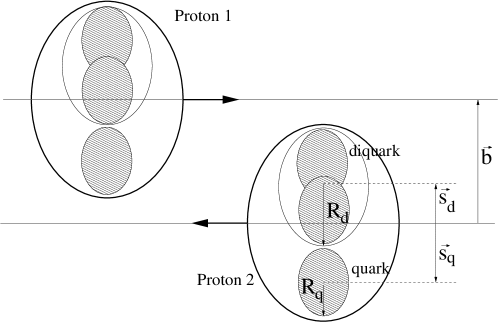
Figure 2: The scattering situation of the two protons when the diquark is assumed to be composed of two quarks, and the proton symbolically can be written as p=(q,(qq)).

If the diquark has the internal structure (11) then the $\sigma_{qd}$, $\sigma_{dq}$ and $\sigma_{dd}$ inelastic differential cross sections (4) can be calculated from $\sigma_{qq}$ using an expansion analogous to expression (3). The results for $\sigma_{qd}$ and $\sigma_{dd}$ are the following [1]

$$\sigma_{qd}\left(\vec{s}\right)=\frac{4A_{qq}R^{2}_{q}}{R^{2}_{d}+R^{2}_{q}}e^{-s^{2}\frac{1}{R^{2}_{d}+R^{2}_{q}}}-\frac{A^{2}_{qq}R^{2}_{q}}{R^{2}_{d}}e^{-s^{2}/R^{2}_{q}},$$ (13)

and

$$\sigma_{dd}\left(\vec{s}\right) =\frac{4A_{qq}R_{q}^{2}}{R_{d}^{2}}e^{-s^{2}\frac{1}{2R_{d}^{2}}}-\frac{4A_{qq}^{2}R_{q}^{4}}{R_{d}^{4}}e^{-s^{2}/R_{d}^{2}}-\frac{2A_{qq}^{2}R_{q}^{2}}{2R_{d}^{2}-R_{q}^{2}}e^{-s^{2}/R_{q}^{2}}+$$ (14)

$$+\frac{4A_{qq}^{3}R_{q}^{4}}{R_{d}^{2}\left(2R_{d}^{2}-R_{q}^{2}\right)}e^{-s^{2}\frac{2R_{d}^{2}+R_{q}^{2}}{2R_{q}^{2}R_{d}^{2}}}-\frac{A_{qq}^{4}R_{q}^{4}}{\left(2R_{d}^{2}-R_{q}^{2}\right)^{2}}e^{-s^{2}\frac{2}{R_{q}^{2}}}.$$

The relevant formula to calculate the inelastic cross section of eq.(1) is again obtained from the expressions summarized in the Appendix.

3 Reproduction and cross-checks of the fits of Bialas and Bzdak

3.1 The diquark acts as a single entity

In this section we reproduce the fitting formula of ref. [1], based on the best values of the model parameters that they have published. These values were obtained in ref. [1] from fitting four essential elements of the elastic scattering cross-sections: they adjusted the model parameters so that (i) the total inelastic cross-section, (ii) the slope of the differential inelastic cross-section at $t=0$, (iii) the position of the diffractive minimum, and (iv) the height of the first diffractive maximum just after the minimum be in agreement with the data. This method lead to remarkable simplicity in the fitting strategy and a very nice, apparent overall agreement with the measured data, as can be seen from the Figures of ref. [1] . As a consequence of this method, the errors of the fit parameters in ref. [1] were not presented, and the overall fit quality parameters ($\chi^{2}$/NDF, CL) were not specified as well, although these are the qualifyers that determine the acceptability of certain models when the language of mathematical statistics is utilized to characterize the data description. By recalculating the original curves, we check in this section the quality of our reproduction of the results of Bialas and Bzdak, and also supplemented their paper with the previously undetermined fit quality parameters.

The results are shown on Figs. 3-6 for the energies $\sqrt{s}=$23.5, 30.7, 52.8, 62.5 GeV respectively. More recently the elastic proton-proton $d\sigma/dt$ was measured by the TOTEM experiment at LHC. The first TOTEM data were published in the $\left|t\right|$ range from 0.36 GeV up to 2.5 GeV [16]. The fit quality parameters presented here are restricted to those data points which fall into this $\left|t\right|$ region, in order to compare the accuracy of the model in the ISR and LHC energy regimes.

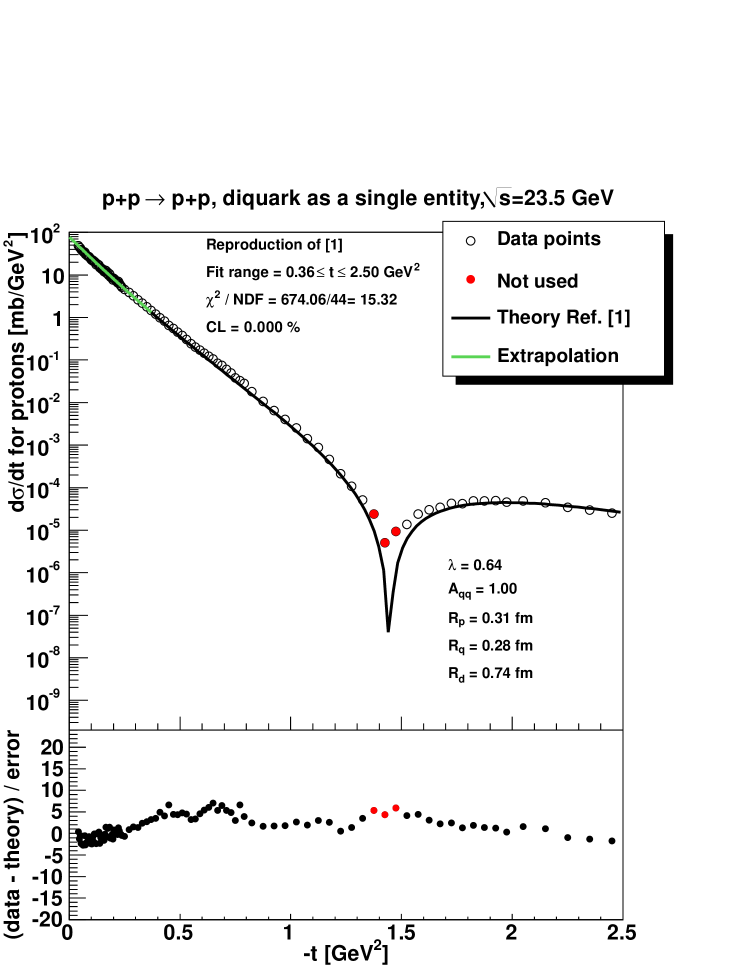
Figure 3: Reproduction of the calculation of A. Bialas and A. Bzdak from [1] at 23.5 GeV, in the case when the diquark is assumed to be a single entity. We have fixed the values of the model parameters to values given in Ref. [1]. In order to determine fit quality, we restricted the fit range to 0.36 GeV $<$ -t $<$ 2.5 GeV, to allow a systematic comparision with more recent TOTEM data at LHC. As the model of Bialas and Bzdak is known to be singular at the dip, in this and all other data analysed we have left out 3 data points from the dip region.

Figure 4: Same as Fig. 3, but at $\sqrt{s}$=30.7 GeV.

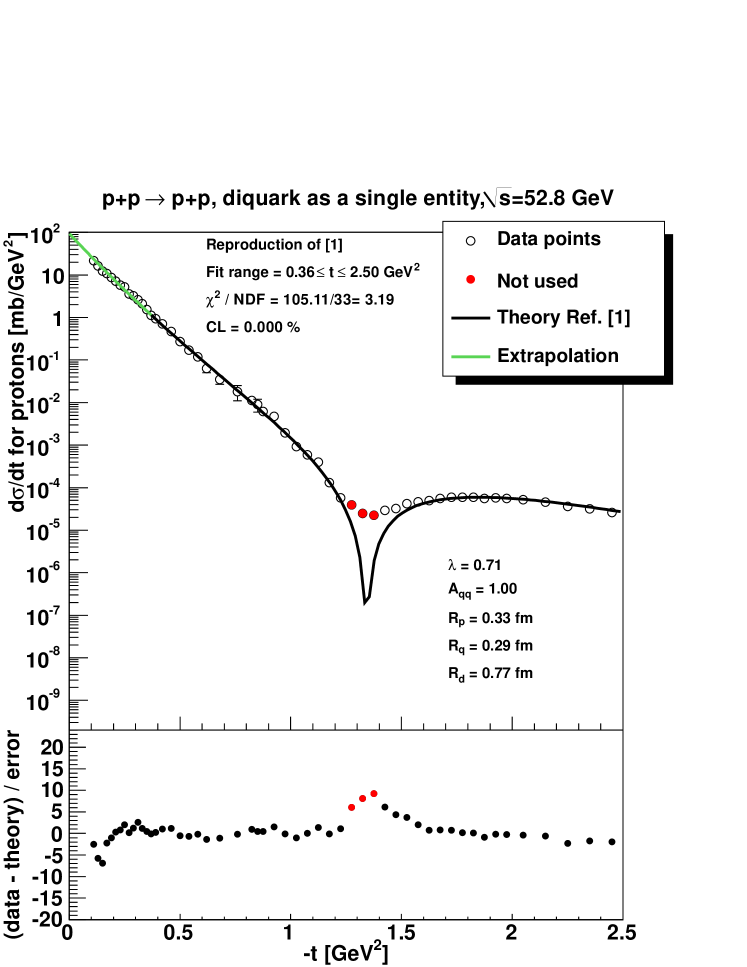
Figure 5: Same as Figs. 3 & 4, at $\sqrt{s}$=52.8 GeV.

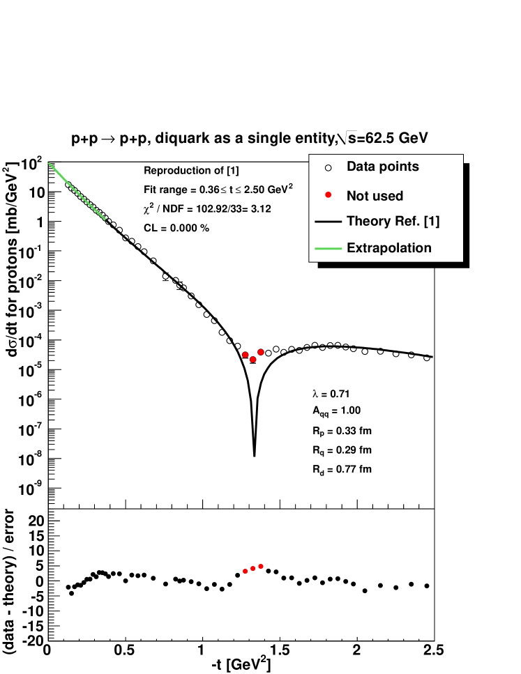
Figure 6: Same as Figs. 3-5, except that the energy is $\sqrt{s}$=62.5 GeV.

3.2 Reproduction of earlier results for the case of composite diquarks

We checked the correctness of our implementation of the formula from the original paper [1]. In the original analysis the errors of the fit parameters were not shown and the overall fit quality parameters ($\chi^{2}$/NDF, CL) are missing as well. The missing fit quality parameters will be supplemented in this section. The results are shown on Fig. 7-10 for the energies 23.5, 30.7, 52.8, 62.5 GeV respectively. More recently the elastic proton-proton $d\sigma/dt$ was measured by the TOTEM experiment at LHC. The first TOTEM data covers the $\left|t\right|$ range from 0.36 GeV up to 2.5 GeV [16]. The fit quality parameters presented here are restricted to those data points which fall into this region, in order to compare the accuracy of the model in the ISR and LHC energy regime.

Figure 7: Reproduction of the calculation of A. Bialas and A. Bzdak [1] at 23.5 GeV, in the case when the diquark is assumed to be a qq entity. We have fixed the values of model parameters to values given in [1]. In order to determine fit quality, we restricted the fit range to 0.36 GeV $<$ -t $<$ 2.5 GeV, to allow a systematic comparision with more recent TOTEM data at LHC. As the model of Bialas and Bzdak is known to be singular at the dip, in this and all other data analysed we have left out 3 data points from the dip region.

Figure 8: Same as Fig 7, except that the analyzed energy is $\sqrt{s}=$ 30.7 GeV.

Figure 9: Same as Fig 7, given at $\sqrt{s}=$ 52.8 GeV.

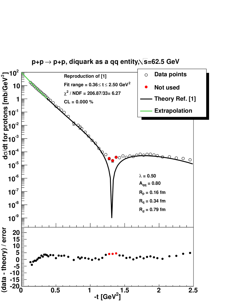
Figure 10: Identical with Fig 7, except that it is evaluated at $\sqrt{s}=$ 62.5 GeV.

4 MINUIT fit results for ISR and TOTEM data

4.1 The diquark acts as a single entity

In this section the MINUIT fit results are presented for the ISR [14, 15] and TOTEM [16] proton-proton elastic scattering data using the single entity model to describe the diquark. Results are illustrated on Fig. 11-15. The confidence levels, and model parameters together with their errors are presented in Table 1, amended with the calculated total elastic cross sections including their uncertainty evaluated from the MINUIT fits. The ratios of the inelastic cross sections were fixed with expression (9) in order to decrease the number of free parameters, therefore these ratios will be provided only for the case when the diquark is assumed to be a composite object.

We have to give some preliminary remarks before presenting the result. The Bialas-Bzdak model shows a singular behaviour at the dip position, having no real part in the amplitude. In order to give a meaning to the fit in this region 3 data points were left out from this dip region during the fit; these points are shown in red on the plots.

Another important remark is that the TOTEM data covers the $|t|$ range from 0.36 GeV up to 2.5 GeV and this range is applied in our minimization procedure to allow a comparison between the ISR and TOTEM results. Note that Bialas and Bzdak adjusted the model to account only for the slope and the value at t = 0 together with the position of the minimum [1]. A different strategy is followed here, since the theoretical curve was fitted directly to the experimental data points using the CERN MINUIT package.

Figure 11: Results of MINUIT fits at ISR energies when the diquark is assumed to be a single entity. The confidence level is higher than 0.1%, which means that the fit quality is acceptable. The fit was mode on the 0.36 - 2.5 GeV $\left|t\right|$ range according to  [16]. As the model is singular around the dip, 3 data points at the dip were left out from the fit. The parameter values are given with statistical errors. The systematic errors are not yet investigated and the effects of the correlation between model parameters are not yet determined, in this sense this result is still preliminary.

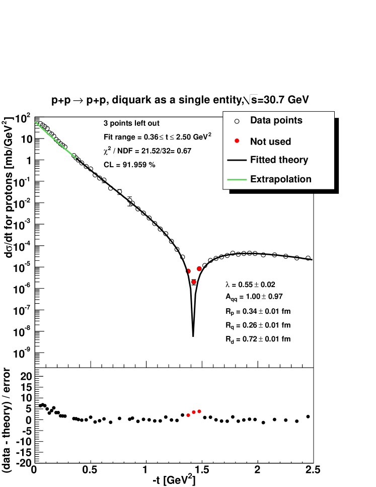
Figure 12: Same as Fig. 11, but for the energy $\sqrt{s}=30.7$ GeV.

Figure 13: Same as Fig. 11, but for the energy $\sqrt{s}=52.8$ GeV.

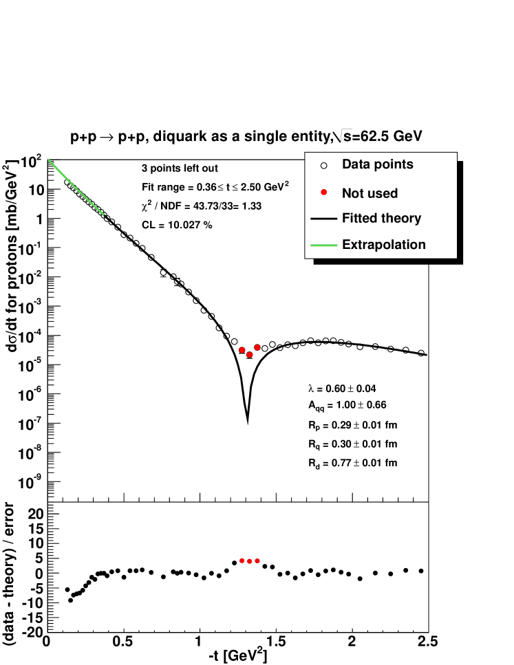
Figure 14: Same as Fig. 11, but for the energy $\sqrt{s}=62.5$ GeV.

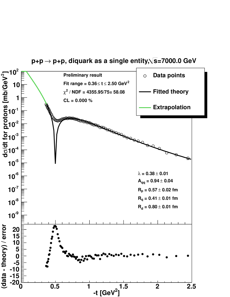
Figure 15: The result of the fit at LHC at $7$ TeV when the diquark is assumed to be one entity. The obtained parameter values are given with statistical errors. Note that CL is below 0.1%, so the quality of this fit is not acceptable.The systematic errors are not yet investigated and the effects of the correlation between model parameters are not yet determined, in these sense this result is still preliminary.

$\sqrt{s}$ [GeV]	23.5	30.7	52.9	62.5	7000
$R_{p}$ [fm]	0.22 $\pm$ 0.01	0.34 $\pm$ 0.01	0.35 $\pm$ 0.01	0.29 $\pm$ 0.01	0.57 $\pm$ 0.02
$R_{q}$ [fm]	0.34 $\pm$ 0.01	0.26 $\pm$ 0.01	0.26 $\pm$ 0.01	0.30 $\pm$ 0.01	0.41 $\pm$ 0.01
$R_{d}$ [fm]	0.71 $\pm$ 0.01	0.72 $\pm$ 0.01	0.73 $\pm$ 0.01	0.77 $\pm$ 0.01	0.80 $\pm$ 0.01
$\lambda$	0.68 $\pm$ 0.03	0.55 $\pm$ 0.02	0.56 $\pm$ 0.03	0.60 $\pm$ 0.04	0.38 $\pm$ 0.01
$A_{qq}$	0.57 $\pm$ 0.01	1.00 $\pm$ 0.97	1.00 $\pm$ 0.80	1.0 $\pm$ 0.66	0.94 $\pm$ 0.04
$\chi^{2}/NDF$	60.6/44	21.5/32	50.2/33	43.73/33	4355.9/75
$CL$ [%]	4.9	92.0	2.8	10.0	0.0
$\sigma^{elastic}_{total}$ [mb]	6.0	5.6	5.9	8.7	20.3

Table 1: The overall fit quality and resulting parameters of the fit at ISR energies including the LHC result at $7$ TeV. The diquark is assumed to be a single entity. The obtained parameter values are given with statistical errors. The systematic errors are not yet investigated and the effects of the correlation between model parameters are not yet determined, so these results in this sense are preliminary.

4.2 The diquark is assumed to be a composite object

In this section the MINUIT results are presented for the ISR [14, 15]

and TOTEM [16] proton-proton elastic scattering data using the assumption that the diquark is a composite qq object. The results are illustrated on Fig. 16-20. The confidence levels, and model parameters with their errors are summarized in Table 2.

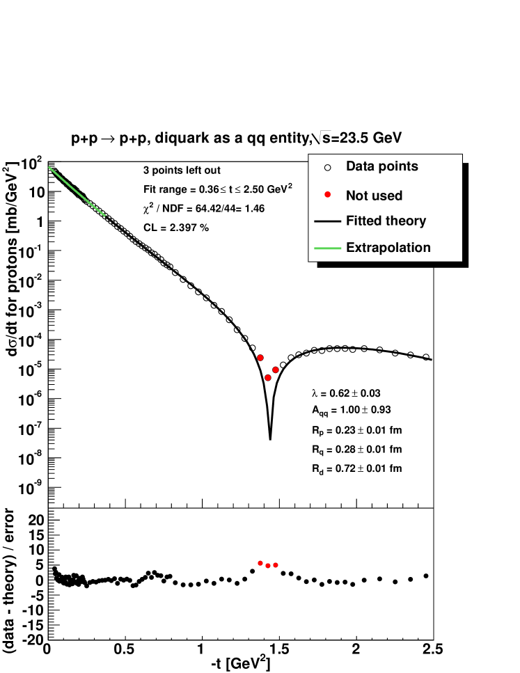
Figure 16: The result of the fit at the 23.5 GeV ISR energy when the diquark is assumed to be a composite entity. The confidence level is higher than 0.1%, which means that the fit quality is acceptable. The fit was mode on the 0.36 - 2.5 GeV $\left|t\right|$ range according to  [16]. As the model is singular around the dip, 3 data points at the dip were left out from the fit. The parameter values are given with statistical errors. The systematic errors are not yet investigated and the effects of the correlation between model parameters are not yet determined, in this sense this fit result is still preliminary.

Figure 17: Same as Fig 16, except that it is provided for $\sqrt{s}=$ 30.7 GeV.

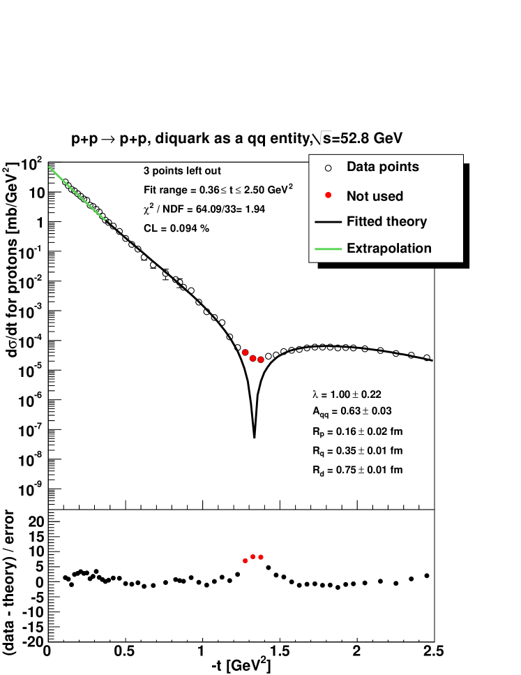
Figure 18: Same as Fig 16, given for $\sqrt{s}=$ 52.8 GeV.

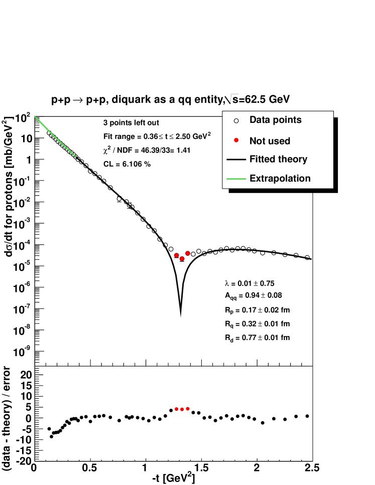
Figure 19: Same as Fig 16, calculated for $\sqrt{s}=$ 62.5 GeV.

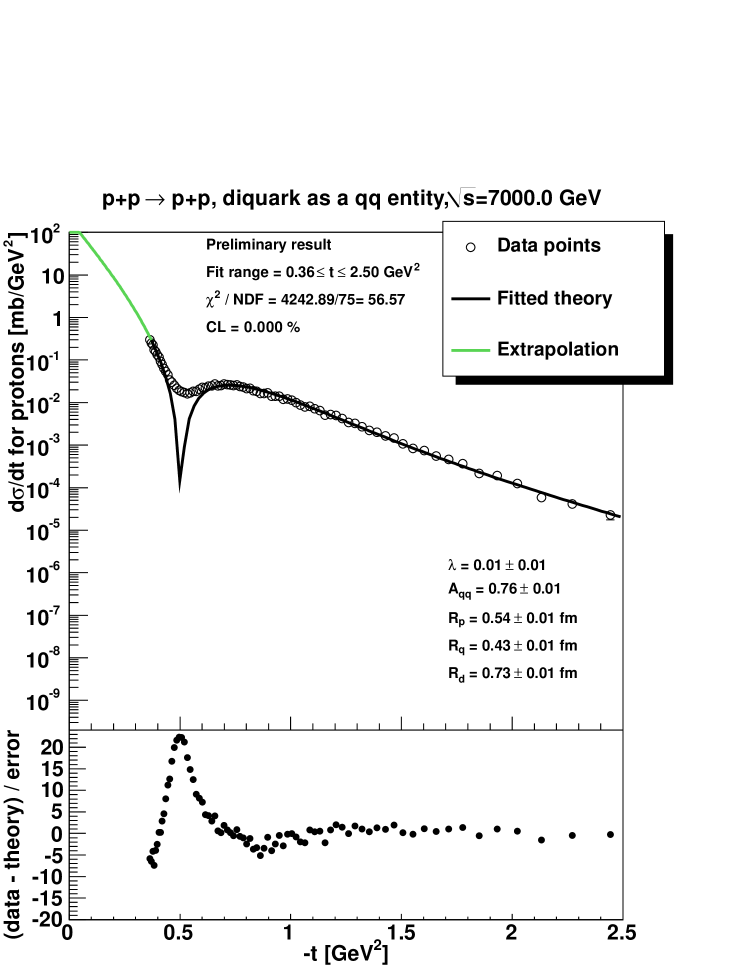
Figure 20: Same as Fig 16, but for $\sqrt{s}=$ 7 TeV. Note that this fit is not acceptable since CL is below 0.1%.

$\sqrt{s}$ [GeV]	23.5	30.6	52.9	62.5	7000
$R_{p}$ [fm]	0.23 $\pm$ 0.01	0.18 $\pm$ 0.02	0.16 $\pm$ 0.02	0.17 $\pm$ 0.02	0.54 $\pm$ 0.01
$R_{q}$ [fm]	0.28 $\pm$ 0.01	0.34 $\pm$ 0.01	0.35 $\pm$ 0.01	0.32 $\pm$ 0.01	0.43 $\pm$ 0.01
$R_{d}$ [fm]	0.72 $\pm$ 0.01	0.73 $\pm$ 0.01	0.75 $\pm$ 0.01	0.77 $\pm$ 0.01	0.73 $\pm$ 0.01
$\lambda$	0.62 $\pm$ 0.03	1.00 $\pm$ 0.64	1.00 $\pm$ 0.22	0.01 $\pm$ 0.75	0.01 $\pm$ 0.01
$A_{qq}$	1.00 $\pm$ 0.93	0.65 $\pm$ 0.03	0.63 $\pm$ 0.03	0.94 $\pm$ 0.08	0.76 $\pm$ 0.01
$\chi^{2}/NDF$	64.42/44	30.42/32	64.1/33	46.4/33	4242.9/75
$CL$ [%]	2.40	54.6	0.1	6.1	0.0
$\sigma^{elastic}_{total}$ [mb]	6.5	6.0	6.4	8.4	13.1

Table 2: The overall fit quality and resulting parameters of the fit at the ISR energies including the LHC result at $7$ TeV. The diquark is a assumed to be a qq entity. The obtained parameter values are given with statistical errors. The systematic errors are not yet investigated and the effects of the correlation between model parameters are not yet determined, so these results are preliminary.

4.3 Total cross sections in the composite diquark model

The total inelastic cross sections for the quark-quark, quark-diquark and diquark-diquark subcollisions were analysed according to formula (4). The detailed results are collected in Table 3, while the average ratios for the described ISR energies are

$\sqrt{s}$ [GeV]	23.5	30.6	52.9	62.5	7000
$\sigma_{qd}/\sigma_{qq}$	1.92 $\pm$ 0.08	1.93 $\pm$ 0.01	1.93 $\pm$ 0.01	1.92 $\pm$ 0.01	1.87 $\pm$ 0.01
$\sigma_{dd}/\sigma_{qq}$	3.64 $\pm$ 0.34	3.66 $\pm$ 0.03	3.67 $\pm$ 0.03	3.61 $\pm$ 0.05	3.38 $\pm$ 0.02

Table 3: The ratios of the total inelastic cross sections for the quark-quark, quark-diquark and diquark-diquark processes for the ISR and LHC energies using the composite diquark hypothesis.

$$\sigma_{qq}:\sigma_{qd}:\sigma_{dd}=1:(1.93\pm 0.03):(3.64\pm 0.1),$$ (15)

which is close to the ideal 1: 2 : 4 ratio, confirming the assumption of having two quarks inside the diquark, amended with some shadowing which is 3.5% and 9% respectively. At 7 TeV the ratios are slightly different from (15)

$$1:(1.87\pm 0.01):(3.38\pm 0.02),$$ (16)

which shows that the shadowing is stronger, 6.5% and 16% percent respectively.

The total elastic scattering cross sections were also determined, as given in Table 2. Note, that the errors on the total cross-section have not yet been obtained reliably at this point. The reason is that the errors of total cross-sections are very strongly correlated with the errors of $A_{qq}$. However the current fits cannot determine precisely the value of this parameter: its nearly 100 % relative error indicates the approximate insensitivity of the results on this value. Hence one has to study the possibility of fixing this and also the parameters like $\lambda$ to reasonable values and to see if in such scenarios the quality of the results remains the same or not.These studies and the final values of the total elastic scattering cross-sections will be submitted for a separate publication.

5 Conclusion and outlook

A systematic study of fit quality as well as the fit parameters under similar circumstances has been performed for the Bialas - Bzdak model in a wide energy range from ISR to LHC energies. The model gives a good description of the ISR data, which means that the CL is acceptable on the ISR energies if 3 data points at the dip were left out from the fit. The total proton-proton cross section (“size” of the proton) clearly seems to grow with energy but the model fails at this energy domain as CL is not acceptable at $7$ TeV. This preliminary result does not include systematics, and the correlation between the fit parameters are still under investigation.

An important shortcoming of the quark-diquark model of protons is that it ignores the real part of the elastic scattering amplitude. This leads to a singular behaviour at the diffractive minimum, which is apparently a more and more serious model limitation with increasing the energy of the p+p collisions.

The evaluated ratios of the quark-quark, quark-diquark and diquark-diquark total inelastic cross-sections were found to deviate more and more from the ideal 1 : 2 : 4 ratio with increasing energies. In the ISR energy range the deviations from this ideal value were not yet significant, indicating lack of significant shadowing effects. However at the current LHC energy of $\sqrt{s}=7$ TeV, a significant decrease compared to these ideal ratios were found, which possibly may indicate an increased role of shadowing at CERN LHC energies.

The final conclusions of this study will be summarized separately and submitted for a publication. The current status corresponds to the level of our understanding around September 2011, at the time of the 2011 Summer School on Diffraction in Heidelberg, where these results were first presented.

Finally let us note that the TOTEM Collaboration extended recently the measurement of the differential elastic p+p scattering cross-sections to low values of $|t|$ in ref. [17], allowing one to extrapolate to the optical point at $t=0$ and to determine the total elastic and the total scattering cross-sections of p+p collisions at $\sqrt{s}=7$ TeV for the first time, but these data were yet not utilized in our analysis.

As a final remark, at the time of the completion of this conference contribution it is inspiring to see the great theoretical interest in the differential elastic cross-section measurement of TOTEM at LHC, as evidenced by the increasing amount of theoretical interpretations and successfull descriptions of certain aspects of these data. As our contribution is not intended to be a review on the interpretation of TOTEM data, we just would like to call attention to some of the most interesting approaches of describing these measurements as evidenced in refs.  [18, 19, 20, 21, 22, 23, 24, 25].

6 Acknowledgements

T. Csörgő would like to thank prof. R. J. Glauber for valuable discussions at the initial phase of this project, and for his kind hospitality at Harvard University. F.N. would like to thank A. Ster and M. Csanád for their valuable help with the CERN MINUIT multi-parameter optimization.

This research was partially supported by the Hungarian American Enterprize Scholarship Fund (HAESF) and by the Hungarian OTKA grant NK 101438.

7 Appendix

Two of the Dirac $\delta$ functions in (1) induce the following transformation in the transverse diquark and quark position variables

$$\vec{s_{d}}=-\lambda\vec{s_{q}},\,\vec{s_{d}}^{\prime}=-\lambda\vec{s_{q}}^{\prime}.$$ (17)

Hence four Gaussian integration remain, which lead us to the following result

$$\frac{4v^{2}}{\pi^{2}} \int{\text{d}^{2}s_{q}\text{d}^{2}s_{q}^{\prime}e^{-2v\left(s_{q}^{2}+s_{q}^{\prime 2}\right)}e^{-c_{qq}\left(b-s_{q}+s_{q}^{\prime}\right)^{2}}e^{-c_{qd}\left(b-s_{q}+s_{d}^{\prime}\right)^{2}}\times}$$ (18)

$$\times e^{-c_{dq}\left(b-s_{d}+s_{q}^{\prime}\right)^{2}}e^{-c_{dd}\left(b-s_{d}+s_{d}^{\prime}\right)^{2}}=\frac{4v^{2}}{\Omega}e^{-b^{2}\frac{\Gamma}{\Omega}},$$

where the coefficients $c_{ab}$ are abbrevations, and

$$\Omega =\left[4v+\left(1+\lambda\right)^{2}\left(c_{qd}+c_{dq}\right)\right]\left[v+c_{qq}+\lambda^{2}c_{dd}\right]+$$ (19)

$$+\left(1-\lambda\right)^{2}\left[v\left(c_{qd}+c_{dq}\right)+\left(1+\lambda\right)^{2}c_{qd}c_{dq}\right],$$

while

$$\Gamma =\left[4v+\left(1+\lambda\right)^{2}\left(c_{qd}+c_{dq}\right)\right]\left[v\left(c_{qq}+c_{dd}\right)+\left(1+\lambda\right)^{2}c_{qq}c_{dd}\right]+$$ (20)

$$+\left[4v+\left(1+\lambda\right)^{2}\left(c_{qq}+c_{dd}\right)\right]\left[v\left(c_{qd}+c_{dq}\right)+\left(1+\lambda\right)^{2}c_{qd}c_{dq}\right].$$

References

- [1] A. Bialas and A. Bzdak, Acta Phys. Polon. B 38, 159 (2007) [hep-ph/0612038].
- [2] A. Bzdak, Acta Phys. Polon. B 38 (2007) 2665 [hep-ph/0701028].
- [3] A. Bialas and A. Bzdak, Phys. Lett. B 649 (2007) 263 [nucl-th/0611021].
- [4] A. Bialas and A. Bzdak, Phys. Rev. C 77 (2008) 034908 [arXiv:0707.3720 [hep-ph]].
- [5] F. James and M. Roos, Comput. Phys. Commun. 10 (1975) 343.
- [6] A. Adare et al. [PHENIX Collaboration], Phys. Rev. Lett. 103 (2009) 012003 [arXiv:0810.0694 [hep-ex]].
- [7] For a recent summary of the discovery of the exotic hadrons XYZ see the KEK press release at http://www.kek.jp/intra-e/press/2012/011014/ .
- [8] M. Kreps [Belle and Babar Collaborations], PoS BEAUTY 2009 (2009) 038 [arXiv:0912.0111 [hep-ex]].
- [9] A. Bialas, K. Fialkowski, W. Slominski and M. Zielinski, Acta Phys. Polon. B 8, 855 (1977)
- [10] R. J. Glauber, Nucl. Phys. A 774 (2006) 3 [nucl-th/0604021].
- [11] R. J. Glauber, Lectures in Theoretical Physics, ed. W. E. Brittin and L. G. Dunham (Interscience Publishers, New York, 1959), vol. 1, p. 315.
- [12] R. J. Glauber, Phys. Rev. 100 (1955) 242.
- [13] W. Czyz and L. C. Maximon, Annals Phys. 52 (1969) 59.
- [14] E. Nagy, R. S. Orr, W. Schmidt-Parzefall, K. Winter, A. Brandt, F. W. Busser, G. Flugge and F. Niebergall et al., Nucl. Phys. B 150 (1979) 221.
- [15] U. Amaldi and K. R. Schubert, Nucl. Phys. B 166 (1980) 301.
- [16] G. Antchev et al. [TOTEM Collaboration], Europhys. Lett. 95, 41001 (2011) [arXiv:1110.1385 [hep-ex]].
- [17] G. Antchev, P. Aspell, I. Atanassov, V. Avati, J. Baechler, V. Berardi, M. Berretti and E. Bossini et al., Europhys. Lett. 96 (2011) 21002 [arXiv:1110.1395 [hep-ex]].
- [18] D. A. Fagundes, E. G. S. Luna, M. J. Menon and A. A. Natale, arXiv:1108.1206 [hep-ph].
- [19] A. D. Martin, M. G. Ryskin and V. A. Khoze, arXiv:1110.1973 [hep-ph].
- [20] T. Wibig, arXiv:1111.0441 [hep-ph].
- [21] V. Uzhinsky and A. Galoyan, arXiv:1111.4984 [hep-ph].
- [22] A. Donnachie and P. V. Landshoff, arXiv:1112.2485 [hep-ph].
- [23] D. A. Fagundes, E. G. S. Luna, M. J. Menon and A. A. Natale, arXiv:1112.4680 [hep-ph].
- [24] M. M. Block and F. Halzen, arXiv:1201.0960 [hep-ph].
- [25] M. G. Ryskin, A. D. Martin and V. A. Khoze, arXiv:1201.6298 [hep-ph].