Spherical Solutions due to the Exterior Geometry of a Charged Weyl Black Hole

Abstract

Firstly we derive peculiar spherical Weyl solutions, using a general spherically symmetric metric due to a massive charged object with definite mass and radius. Afterwards, we present new analytical solutions for relevant cosmological terms, which appear in the metrics. Connecting the metrics to a new geometric definition of a charged Black Hole, we numerically investigate the effective potentials of the total dynamical system, considering massive and massless test particles, moving on such Black Holes.

¹Department of Physics, Payame Noor University, PO BOX 19395-3697, Tehran, Iran

²Department of Physics, Islamic Azad University, Central Tehran Branch, Tehran, Iran

1 Introduction

Among generalized theories of gravity, Weyl gravity is remarkable, since it leads to considerable descriptions of cosmological parameters relevant to Dark Energy problem. It is known that Weyl theory, contributes in the $R^{2}$ theories of gravity. This means that this theory is governed by field equations, combined of second order differentiations of the Ricci scalar [1]:

$$W_{\alpha\beta}=\nabla^{\rho}\nabla_{\alpha}R_{\beta\rho}+\nabla^{\rho}\nabla_{\beta}R_{\alpha\rho}-\Box R_{\alpha\beta}-g_{\alpha\beta}\nabla_{\rho}\nabla_{\lambda}R^{\rho\lambda}$$

$$-2R_{\rho\beta}R^{\rho}_{\alpha}+\frac{1}{2}g_{\alpha\beta}R_{\rho\lambda}R^{\rho\lambda}-\frac{1}{3}\Big{(}2\nabla_{\alpha}\nabla_{\beta}R-2g_{\alpha\beta}\Box R-2RR_{\alpha\beta}+\frac{1}{2}g_{\alpha\beta}R^{2}\Big{)}=\frac{1}{4\pi}T_{\alpha\beta}.$$ (1)

In the above equation, $W_{\alpha\beta}$ notates the components of the Weyl equations, and $T_{\alpha\beta}$ is the energy momentum tensor, corresponding to the source. The vacuum equations, generally have been solved and a spherically symmetric metric has been derived [2]. In this paper, we are not concerning about the general solution. Instead, we consider a peculiar one, that corresponds to a massive charged spherically symmetric source. Such source has been considered for the Reissner-Nordström solutions (RN) of Weyl gravity [3], but here we use the background field method and linear approximation to derive other RN-like solutions, also describing a charged Black Hole. The method is like the one, which has done in [4], analytically investigating the constants regarding the Dark Energy problem. However here, constant values of charge and mass will be considered, to rearrange the metric to a new form to describe a Black Hole. Finally, the effective potentials will be numerically plotted to illustrate the geometric behavior of the dynamical system, affected by such Black Hole.

2 A spherical solution of Weyl field equations due to a charged massive spherical source

Let us consider the following general metric:

$$ds^{2}=-\Big{(}1-\frac{2GM}{r}-\frac{1}{3}f(r)\Big{)}dt^{2}+\Big{(}1-\frac{2GM}{r}-\frac{1}{3}f(r)\Big{)}^{-1}dr^{2}+r^{2}d\Omega^{2},$$ (2)

in which $f(r)$ is an arbitrary $r$-dependent function, ought to be obtained. The Ricci tensor components, due to the spacetime, defined by metric (2) will be:

$$\begin{array}[]{l}R_{00}=\left(-{r}^{2}+2\,Gmr+\frac{1}{3}\,f{r}^{2}\right)\times\\ \left(\frac{1}{12}\,{\frac{\left({\it f^{\prime}}\,{r}^{2}+2\,fr\right)^{2}}{f}}+\frac{1}{3}\,\sqrt{3}\sqrt{f{r}^{2}}\left(-\frac{1}{12}\,{\frac{\sqrt{3}\left({\it f^{\prime}}\,{r}^{2}+2\,fr\right)^{2}}{\left(f{r}^{2}\right)^{\frac{3}{2}}}}+\frac{1}{6}\,{\frac{\sqrt{3}\left({\it f^{\prime\prime}}\,{r}^{2}+4\,{\it f^{\prime}}\,r+2\,f\right)}{\sqrt{f{r}^{2}}}}\right){r}^{2}-\frac{1}{3}\,\left({\it f^{\prime}}\,{r}^{2}+2\,fr\right)r+\frac{1}{3}\,f{r}^{2}\right){r}^{-6},\\ \\ R_{11}=-\left(\frac{1}{12}\,{\frac{\left({\it f^{\prime}}\,{r}^{2}+2\,fr\right)^{2}}{f}}+\frac{1}{3}\,\sqrt{3}\sqrt{f{r}^{2}}\left(-\frac{1}{12}\,{\frac{\sqrt{3}\left({\it f^{\prime}}\,{r}^{2}+2\,fr\right)^{2}}{\left(f{r}^{2}\right)^{\frac{3}{2}}}}+\frac{1}{6}\,{\frac{\sqrt{3}\left({\it f^{\prime\prime}}\,{r}^{2}+4\,{\it f^{\prime}}\,r+2\,f\right)}{\sqrt{f{r}^{2}}}}\right){r}^{2}-\frac{1}{3}\,\left({\it f^{\prime}}\,{r}^{2}+2\,fr\right)r+\frac{1}{3}\,f{r}^{2}\right){r}^{-2}\\ \times\left(-{r}^{2}+2\,Gmr+\frac{1}{3}\,f{r}^{2}\right)^{-1},\\ \\ R_{22}=-\frac{1}{3}\,\sqrt{3}\sqrt{f{r}^{2}}\left(-\frac{1}{3}\,{\frac{\sqrt{3}\left({\it f^{\prime}}\,{r}^{2}+2\,fr\right)r}{\sqrt{f{r}^{2}}}}+\frac{1}{3}\,\sqrt{3}\sqrt{f{r}^{2}}\right){r}^{-2},\\ \\ R_{33}=R_{22}\sin^{2}(\theta).\end{array}$$ (3)

Also the Ricci scalar will be derived as:

$$R=\frac{1}{3}\,{\frac{{\it f^{\prime\prime}}\,{r}^{2}+4\,{\it f^{\prime}}\,r+2\,f}{{r}^{2}}}.$$ (4)

Employing these values in the components of Weyl equations in (1), one obtains:

$$\begin{array}[]{l}W_{00}={\frac{1}{324}}\,{r}^{-5}\Big{(}72\,{\it f^{\prime}}\,{r}^{2}-72\,\left(f\right)r-24\,Gm{{\it f^{\prime}}}^{2}{r}^{2}+288\,Gm{\it f^{\prime\prime}}\,{r}^{2}-6\,Gm{{\it f^{\prime\prime}}}^{2}{r}^{4}-432\,r{G}^{2}{m}^{2}{\it f^{\prime\prime}}\\ -360\,Gm{\it f^{\prime}}\,r+360\,{r}^{2}{G}^{2}{m}^{2}{\it f^{\prime\prime\prime}}-12\,{{\it f^{\prime}}}^{2}{r}^{3}+4\,{f}^{3}r+36\,{\it f^{\prime\prime}}\,{r}^{3}-36\,{r}^{5}{\it f^{\prime\prime\prime\prime}}-108\,{r}^{4}{\it f^{\prime\prime\prime}}\\ -3\,{{\it f^{\prime\prime}}}^{2}{r}^{5}-120\,Gm{\it f^{\prime}}\,r\left(f\right)-12\,{r}^{4}Gm{\it f^{\prime}}\,{\it f^{\prime\prime\prime}}-132\,{r}^{3}\left(f\right)Gm{\it f^{\prime\prime\prime}}+96\,Gm\left(f\right){\it f^{\prime\prime}}\,{r}^{2}\\ -48\,{r}^{4}Gm\left(f\right){\it f^{\prime\prime\prime\prime}}-24\,Gm{\it f^{\prime}}\,{r}^{3}{\it f^{\prime\prime}}-2\,{r}^{5}\left(f\right){\it f^{\prime\prime\prime}}\,{\it f^{\prime}}+396\,{r}^{3}{\it f^{\prime\prime\prime}}\,Gm-144\,{r}^{3}{G}^{2}{m}^{2}{\it f^{\prime\prime\prime\prime}}\\ +144\,{r}^{4}{\it f^{\prime\prime\prime\prime}}\,Gm-4\,\left(f\right){r}^{4}{\it f^{\prime}}\,{\it f^{\prime\prime}}+12\,{\it f^{\prime}}\,{r}^{4}{\it f^{\prime\prime}}+24\,{r}^{5}{\it f^{\prime\prime\prime\prime}}\,\left(f\right)+72\,{r}^{4}\left(f\right){\it f^{\prime\prime\prime}}-4\,{r}^{5}{f}^{2}{\it f^{\prime\prime\prime\prime}}\\ -12\,{r}^{4}{f}^{2}{\it f^{\prime\prime\prime}}+24\,Gm{f}^{2}+4\,\left(f\right){r}^{3}{{\it f^{\prime}}}^{2}-8\,{f}^{2}{r}^{2}{\it f^{\prime}}+48\,{\it f^{\prime}}\,{r}^{2}\left(f\right)-144\,Gm\left(f\right)+6\,{\it f^{\prime}}\,{r}^{5}{\it f^{\prime\prime\prime}}\\ -24\,{r}^{3}\left(f\right){\it f^{\prime\prime}}+\left(f\right){r}^{5}{{\it f^{\prime\prime}}}^{2}-432G^{2}m^{2}f^{\prime}\Big{)},\\ \\ W_{11}=-\frac{1}{36}\,{\frac{1}{{r}^{3}\left(-3\,r+6\,Gm+\left(f\right)r\right)}}\Big{(}-4\,{r}^{3}{\it f^{\prime\prime\prime}}\,\left(f\right)+24\,f+12\,{\it f^{\prime\prime}}\,{r}^{2}-24\,{\it f^{\prime}}\,r\\ -4\,{{\it f^{\prime}}}^{2}{r}^{2}-4\,{f}^{2}+8\,{\it f^{\prime}}\,r\left(f\right)+2\,{\it f^{\prime}}\,{r}^{4}{\it f^{\prime\prime\prime}}-72\,r{\it f^{\prime\prime}}\,Gm\\ +4\,{r}^{3}{\it f^{\prime}}\,{\it f^{\prime\prime}}-4\,\left(f\right){\it f^{\prime\prime}}\,{r}^{2}-36\,{r}^{2}{\it f^{\prime\prime\prime}}\,Gm-{{\it f^{\prime\prime}}}^{2}{r}^{4}+72\,Gm{\it f^{\prime}}\Big{)},\\ \\ W_{22}=-{\frac{1}{108r^{2}}}\,\Big{(}-24\,{\it f^{\prime}}\,r-4\,{f}^{2}+8\,{\it f^{\prime}}\,r\left(f\right)+72\,Gm{\it f^{\prime}}\\ -4\,\left(f\right){\it f^{\prime\prime}}\,{r}^{2}+2\,{r}^{4}\left(f\right){\it f^{\prime\prime\prime\prime}}+4\,{r}^{3}{\it f^{\prime\prime\prime}}\,\left(f\right)+4\,{r}^{3}{\it f^{\prime}}\,{\it f^{\prime\prime}}\\ +2\,{\it f^{\prime}}\,{r}^{4}{\it f^{\prime\prime\prime}}+12\,{\it f^{\prime\prime}}\,{r}^{2}-4\,{{\it f^{\prime}}}^{2}{r}^{2}-{{\it f^{\prime\prime}}}^{2}{r}^{4}-6\,{r}^{4}{\it f^{\prime\prime\prime\prime}}\\ -12\,{r}^{3}{\it f^{\prime\prime\prime}}-72\,r{\it f^{\prime\prime}}\,Gm+12\,{r}^{3}{\it f^{\prime\prime\prime\prime}}\,Gm+24\,f\Big{)}={\frac{W_{33}}{\sin^{2}(\theta)}}.\end{array}$$ (5)

As we expect,

$$W^{\alpha}_{\alpha}=0.$$

All the components in (5), have a vacuum solution like:

$$f(r)=-c_{1}r^{2}-c_{2}r-\frac{6GM}{r}.$$ (6)

Substituting (6) in (2) yields:

$$ds^{2}=-\Big{(}1+\frac{1}{3}{c_{2}}{r}+\frac{1}{3}c_{1}r^{2}\Big{)}dt^{2}+\Big{(}1+\frac{1}{3}{c_{2}}{r}+\frac{1}{3}c_{1}r^{2}\Big{)}^{-1}dr^{2}+r^{2}d\Omega^{2}.$$ (7)

Now to evaluate the included constants in (6), we shall use the background field method in the weak field limit. The zero-zero component of the metric (2) can be rewritten as:

$$g_{00}=\eta_{00}+h_{00},$$

for small fluctuations $h_{00}=\frac{2GM}{r}+\frac{1}{3}f(r)$. The $r$-component of the Poisson’s equation implies that:

$$\nabla^{2}h_{00}\equiv(\frac{d^{2}}{dr^{2}}+\frac{2}{r}\frac{d}{dr})h_{00}=8\pi\Big{(}T_{00}+E_{00}\Big{)},$$ (8)

in which $T_{00}$ is the stress-energy tensor due to the mass of the source. And here, associated to a charged, spherically symmetric massive source, the tensor is the volume density:

$$T_{00}=\rho_{0}=\frac{m_{0}}{\frac{4}{3}\pi r_{0}^{3}}.$$ (9)

In (9), $m_{0}$ is the mass of the spherical body and $r_{0}$ is its known radius. In relation (8), $E_{00}$ is the stress-energy tensor, associated to the charge amount of the massive object. Here, since the source is assumed to be static, we take the vector potential $A_{\mu}=(\Phi(r),0,0,0)$, where $\Phi(r)$ is the electric potential at point $r$ in the exterior geometry of the total charge $q_{0}$, distributed in a certain volume ($\Phi(r)=\frac{q_{0}}{r}$). We have [5]:

$$E_{00}=\frac{1}{8\pi}\Big{(}\frac{q_{0}}{r^{2}}\Big{)}^{2}+\frac{1}{4\pi}\frac{\partial}{\partial r}\Big{(}\Phi(r)\times\frac{q_{0}}{r^{2}}\Big{)}=\frac{1}{8\pi}\frac{q_{0}^{2}}{r^{4}}.$$ (10)

Now considering the expression (6), and the values in (9), (10) in (8), and solving for $c_{1}$ or $c_{2}$ yields:

$$c_{1}=-3\,{\frac{m_{0}}{{r_{0}}^{3}}}-\frac{1}{2}\,{\frac{\left(q_{0}\right)^{2}}{{r}^{4}}}-\frac{1}{3}\,\frac{c_{2}}{r}.$$ (11)

$$c_{2}=-9\,{\frac{rm_{0}}{{r_{0}}^{3}}}-\frac{3}{2}\,{\frac{\left(q_{0}\right)^{2}}{{r}^{3}}}-3\,{c_{1}}\,r.$$ (12)

considering (12) we get:

$$g_{00}^{(1)}=-(1-\frac{3r^{2}m_{0}}{{r_{0}}^{3}}-\frac{1}{2}\frac{(q_{0})^{2}}{r^{2}}-\frac{2}{3}c_{1}r^{2}).$$ (13)

The general spherically symmetric solution to Weyl gravity, has been derived to be [2]:

$$g^{W}_{00}=-(1-\frac{\beta(2-3\beta\gamma)}{r}-3\beta\gamma+\gamma r-kr^{2}),$$ (14)

in which, as it has been mentioned by the authors, the parameters $\gamma$ and $k$ have been considered to be relevant to the Dark Energy theory. The term $\frac{2}{3}c_{1}r^{2}$ in (13), therefore can be corresponded to the term $kr^{2}$ in (14). To estimate a value for $c_{1}$, we use (11). We consider the characteristics of the observable universe, $m_{0}=m_{\small{obs}}=8\times 10^{55}\,\,\,gr$, and $r_{0}=r_{\small{obs}}=4.39\times 10^{28}\,\,\,cm$, which are respectively, the estimated mass and radius of the observable universe. We also take $q_{0}=q_{\small{obs}}=0$, because it is assumed that a finite universe must have a zero net charge [6]. Taking $c_{2}=0$ in (11) one obtains:

$$c_{1}=\frac{3m_{obs}}{{r_{obs}}^{3}}\approx 2.8\times 10^{-30}\,\,gr/cm^{3},$$

which is comparable to the estimated value for the cosmological constant (see [4] and Ref.s therein).

Now let us consider (11) to obtain:

$$g_{00}^{(2)}=-(1-\frac{r^{2}m_{0}}{{r_{0}}^{3}}-\frac{1}{6}\frac{(q_{0})^{2}}{r^{2}}+\frac{2}{9}c_{2}r).$$ (15)

Looking at (15), leads us to correspond the term $\frac{2}{9}c_{2}r$ to $\gamma r$ in (14). Once more we use the characteristics of the observable universe in (12). Taking $c_{1}=0$ and $r=r_{obs}$ we obtain:

$$c_{2}=\frac{9M}{{r_{obs}}^{2}}\approx 0.3736\,\,gr/{cm}^{2}\equiv 2\times 10^{-28}\,\,cm^{-1}.$$

And this is exactly the value for $\gamma$ which has been presented in [2], related to the Dark Energy theory. In comparison with the Reissner-Nordström-de Sitter metric

$$g_{00}^{RN-d}=-(1-\frac{2m_{0}}{r}+\frac{(q_{0})^{2}}{r^{2}}-\frac{1}{3}\Lambda r^{2}),$$ (16)

the metric (13) shows important differences. Specially when we notice its attractive inverse square potential due to the charged body, instead of the repulsive one in (16). Both of these metrics, have the vacuum energy term, related to the accelerated expansion of the universe. However, the term in (16) would be exactly the cosmological constant, and the one in (13) will have the same value in some limits. On the other hand, the metric in (15) appears to contain another term, which has been not included by common spherically symmetric solutions to Einstein field equations. This term, also by imposing some limits, leads to the same values for the Dark Energy term, in the general spherically symmetric solutions to Weyl gravity.

We will continue our discussion, investigating the effective potentials for the geometrical Black Holes, defined by metrics (13) and (15), without the Dark Energy terms.

3 Effective potentials for a massive charged object around a charged Weyl Black Hole

Considering a test particle, having the characteristics, $m$ for mass and $q$ for charge, which is moving on a Weyl Black Hole, one can derive the effective potential, using the Hamilton-Jacobi equation of wave crests [7, 8]:

$$g^{\mu\nu}(P_{\mu}+qA_{\mu})(P_{\nu}+qA_{\nu})+m^{2}=0.$$ (17)

$P_{\mu}$ is the momentum 4-vector

$$P_{\mu}=g_{\mu\sigma}P^{\sigma}=g_{\mu\sigma}\frac{dx^{\sigma}}{d\lambda}.$$ (18)

where $\lambda$ is the geodesics affine parameter. The metric components $g_{\mu\nu}$ are derived from the exterior geometry of the source, namely metric (13) and (15) without the cosmological terms. Also the vector potential $A_{\mu}$ for our static charged source has been previously defined to be:

$$A_{\mu}=(\Phi(r),0,0,0),$$ (19)

where $\Phi(r)=\frac{q_{0}}{r}$ is the scalar electrical potential, outside the Black Hole. One can define the two conserved quantities as:

$$E=-P_{0},$$ (20)

which is the test-particle’s energy, and

$$L=P_{\phi}\,\,\,\,\,\,\,(L\geq 0).$$ (21)

which is its angular momentum. We choose $\theta=\frac{\pi}{2}$, for which the particle’s motion is confined to the equatorial rotations. Therefore

$$P^{\theta}=\frac{d\theta}{d\lambda}=0.$$

Considering (13) in (17) yields:

$$-\frac{(E-\frac{qq_{0}}{r})^{2}}{1-\frac{3r^{2}m_{0}}{{r_{0}}^{3}}-\frac{1}{2}\frac{{q_{0}}^{2}}{r^{2}}}+(1-\frac{3r^{2}m_{0}}{{r_{0}}^{3}}-\frac{1}{2}\frac{{q_{0}}^{2}}{r^{2}})^{-1}(\frac{dr}{d\lambda})^{2}+\frac{L^{2}}{r^{2}}+m^{2}=0,$$

or

$$(\frac{dr}{d\lambda})^{2}=(E-\frac{qq_{0}}{r})^{2}-(1-\frac{3r^{2}m_{0}}{{r_{0}}^{3}}-\frac{1}{2}\frac{{q_{0}}^{2}}{r^{2}})(m^{2}+\frac{L^{2}}{r^{2}}).$$ (22)

Equation (22) can be rewritten as [8]:

$$(\frac{dr}{d\lambda})^{2}=[E-\big{(}\frac{qq_{0}}{r}-\sqrt{(1-\frac{3r^{2}m_{0}}{{r_{0}}^{3}}-\frac{1}{2}\frac{{q_{0}}^{2}}{r^{2}})(m^{2}+\frac{L^{2}}{r^{2}})}\,\,\big{)}][E-\big{(}\frac{qq_{0}}{r}+\sqrt{(1-\frac{3r^{2}m_{0}}{{r_{0}}^{3}}-\frac{1}{2}\frac{{q_{0}}^{2}}{r^{2}})(m^{2}+\frac{L^{2}}{r^{2}})}\,\,\big{)}],$$

from which we define the effective potential as:

$$V_{eff}^{(1)}=\frac{qq_{0}}{r}+\sqrt{(1-\frac{3r^{2}m_{0}}{{r_{0}}^{3}}-\frac{1}{2}\frac{{q_{0}}^{2}}{r^{2}})(m^{2}+\frac{L^{2}}{r^{2}})},$$ (23)

which is the effective potential due to metric (13). We took the positive part to be assured that a positive potential is available. Using the same procedure for (15) yields:

$$V_{eff}^{(2)}=\frac{qq_{0}}{r}+\sqrt{(1-\frac{r^{2}m_{0}}{{r_{0}}^{3}}-\frac{1}{6}\frac{{q_{0}}^{2}}{r^{2}})(m^{2}+\frac{L^{2}}{r^{2}})}.$$ (24)

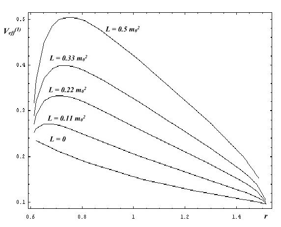
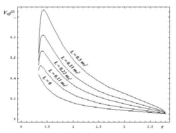
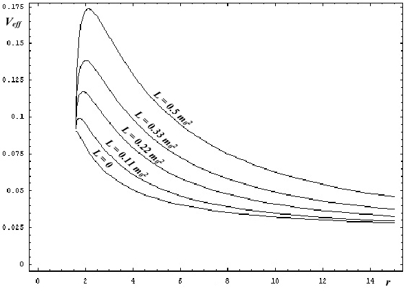
(a) (b) (c)

Figure 1: (a) The effective potentials for a test-particle, having different angular momentums, moving on a charged Weyl Black Hole defined by metric (13) and (b) by metric (15). (c) The effective potentials for a test-particle moving on a Reissner-Nordström (RN) Black Hole.

Figure 1 shows illustrations for these effective potentials for different values of angular momentums.

As charged Black Holes, either of the Weyl Black Holes must have two event horizons for $g_{00}^{(1)}=0$ and $g_{00}^{(2)}=0$. For a Black Hole with a constant radius $r_{0}$ and mass $m_{0}$, one obtains:

$$r_{\pm}^{(1)}=\frac{1}{6}\,{\frac{\sqrt{6m_{{0}}\left({r_{{0}}}^{2}\pm\sqrt{{r_{{0}}}^{4}-6\,m_{{0}}{q_{{0}}}^{2}r_{{0}}}\right)r_{{0}}}}{m_{{0}}}},$$ (25)

$$r_{\pm}^{(2)}=\frac{1}{6}\,{\frac{\sqrt{6m_{{0}}\left(3\,{r_{{0}}}^{2}\pm\sqrt{9\,{r_{{0}}}^{4}-6\,m_{{0}}{q_{{0}}}^{2}r_{{0}}}\right)r_{{0}}}}{m_{{0}}}},$$ (26)

respectively for (13) and (15). Note that, for a Reissner-Nordström Black Hole we have:

$$r_{\pm}^{(RN)}=m_{{0}}\pm\sqrt{{m_{{0}}}^{2}-{q_{{0}}}^{2}}.$$ (27)

In the next section, we restrict our discussion to massless particles.

4 Effective potentials for massless particles travelling on a Weyl Black Hole

For massless particles, namely Photon, Neutrino or Graviton, the characteristics of the test particle changes due to this fact that the concepts of mass and angular momentum, will break down. We shall introduce the ratio [7, 9]:

$$b=\lim_{m\longrightarrow 0}\frac{L}{(E^{2}-m^{2})^{\frac{1}{2}}}.$$ (28)

Previously we defined:

$$g_{\phi\phi}P^{\phi}=L\,\,\,\Rightarrow\,\,\,\frac{d\phi}{d\lambda}=\frac{L}{r^{2}},$$

therefore, according to (28), from Eq. (22) for a massless neutral particle we have:

$$(\frac{1}{r^{2}}\frac{dr}{d\phi})^{2}-\frac{1-\frac{3r^{2}m_{0}}{{r_{0}}^{3}}-\frac{1}{2}\frac{(q_{0})^{2}}{r^{2}}}{r^{2}}=b^{-2}.$$ (29)

We take

$$C_{1}^{-2}=\frac{1-\frac{3r^{2}m_{0}}{{r_{0}}^{3}}-\frac{1}{2}\frac{(q_{0})^{2}}{r^{2}}}{r^{2}},$$

for the Weyl Black Hole, which is defined by (13), and also we take

$$C_{2}^{-2}=\frac{1-\frac{r^{2}m_{0}}{{r_{0}}^{3}}-\frac{1}{6}\frac{(q_{0})^{2}}{r^{2}}}{r^{2}},$$

for the one, defined by (15). Note that, for $b\leq C$, the particle can get to any point $r$. Here, $C^{-2}$ is considered to be the effective potential for the massless particles, moving around a Weyl Black Hole. This means that the maximum, or the critical value for $b$ (we call $b_{crit}$) is the minimum value for $C$. One can derive this critical value for either of Weyl Black Holes. For first type Black Holes, this critical value appears at $r=q_{0}$. We have:

$$b_{crit}^{(1)}=[C_{1}]_{min}={\frac{q_{0}}{\sqrt{\left(\frac{1}{2}-3\,{\frac{{q_{0}}^{2}m_{0}}{{r_{0}}^{3}}}\right){}{}}}}.$$ (30)

Also for the second type Weyl Black Holes, the critical point would be at $r=\frac{q_{0}}{\sqrt{3}}$, and:

$$b_{crit}^{(2)}=[C_{2}]_{min}=\frac{\sqrt{3}}{3}\,{\frac{q_{0}}{\sqrt{\left(\frac{1}{2}-\frac{1}{3}\,{\frac{{q_{0}}^{2}m_{0}}{{r_{0}}^{3}}}\right){}{}}}}.$$ (31)

In Figure 2, the values of effective potentials for a massless particle for both types of Weyl Black Holes, has been plotted.

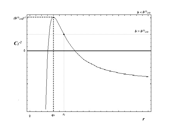
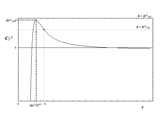
(a) (b)

Figure 2: (a) The effective potentials for a massless test-particle, moving on a first type and (b) second type Weyl Black Hole. $r_{t}$ would be the turning point. For energies higher than the $(b_{crit})^{-2}$, the massless particle is captured by the Black Hole, while for energies lower than this, we have a reflection from the potential well, having the minimum distance $r_{t}.$

When $b$ for either of the massless particles on either of Black Holes, exceeds the $b_{crit}$, then the particle approaches the Black Hole having the minimum distance $r_{t}$, and then goes to infinity. On the maximum of the effective potential, where $b=b_{crit}$, the particle will have unstable circular orbits. For $b<b_{crit}$, the test particle which is coming from infinity, falls into the Black Hole horizon. More details can be found on text books, for example see [10].

5 Conclusion

While Einstein theory of relativity, illustrates a finite classical universe, with a positive acceleration in time like coordinates, some other gravitational theories, are presenting solutions for some unexplained features. In this article one of the most well known ones, namely the Weyl theory of gravity has been considered. Through this theory, we presented some analytical expressions for the coefficients, relevant to Dark Energy theory, and derived their numeric values, which have been in good agreement with their measured values. Also, we specialized the spherically symmetric metrics, explaining the exterior geometry of charged spherical massive source, into two shapes of metric potentials. These time like metrics, having corresponding singularities, described two types of charged Black Holes, in analogy to the Reissner-Nordström metric. Considering them, we calculated the effective potentials for massive and massless test particles and compared them through numerical illustrations.


Acknowledgments
This work was supported under a research grant by Payame Noor University.

References

- [1] D. Kazanas and P.D. Mannheim, General structure of the gravitational equations of motion in conformal Weyl gravity, Astrophysical Journal Supplement Series 76: 431 (1991).
- [2] P.D. Mannheim and D. Kazanas, Exact vacuum solution to conformal Weyl gravity and galactic rotation curves, Astrophysical Journal 342: 635 (1989).
- [3] P.D. Mannheim and D. Kazanas, Solutions to the Reissner-Nordström, Kerr and Kerr- Newman problems in fourth order conformal Weyl gravity, Phys. Rev. D 44, 417(1991).
- [4] M.R. Tanhayi, M. fathi, M.V. Takook, Observable Quantities in Weyl Gravity, Mod. Phys. Lett. A 26, 32(2011).
- [5] J.D. Jackson (1998), Classical Electrodynamics (3rd ed.), Wiley. ISBN 0-471-30932-X.
- [6] L.D. Landau, E.M. Lifshitz, The Classical Theory of Fields. Vol. 2 (4th ed.), Butterworth-Heinemann (1975). ISBN 978-0-750-62768-9.
- [7] C.W. Misner, K.S. Thorne and J.A. Wheeler, Gravitation, Freeman (1973).
- [8] Marco Olivares, Joel Saavedra, J.R. Villanueva and Carlos Leiva, Motion of charged particles on the Reissner-Nordström (Anti)-de Sitter black holes, arXiv:1101.0748v2.
- [9] Bernard F. Schutz, A First Course in General Relativity, Second Edition, Cambridge University Press (2009).
- [10] S. Chandrasekhar, The Mathematical Theory of Black Holes, Oxford University Press, New York (1983).